On the Distribution of Plasmoids In High-Lundquist-Number Magnetic Reconnection

Abstract

The distribution function $f(\psi)$ of magnetic flux $\psi$ in plasmoids formed in high-Lundquist-number current sheets is studied by means of an analytic phenomenological model and direct numerical simulations. The distribution function is shown to follow a power law $f(\psi)\sim\psi^{-1}$, which differs from other recent theoretical predictions. Physical explanations are given for the discrepant predictions of other theoretical models.

In recent years, significant advances have been made in understanding the role of plasmoids (or secondary islands) in magnetic reconnection, which is believed to be the underlying mechanism of energy release for phenomena such as solar flares, magnetospheric substorms, and sawtooth crashes in fusion plasmasZweibel and Yamada (2009). Plasmoids often form spontaneously in resistive magnetohydrodynamics (MHD) Biskamp (1986); Lapenta (2008); Bhattacharjee et al. (2009); Cassak et al. (2009), Hall MHD Shepherd and Cassak (2010); Huang et al. (2011), and kinetic particle-in-cell (PIC) Drake et al. (2006); Daughton et al. (2006, 2009) simulations of large scale reconnection. Evidences of plasmoids have also been found in the magnetotail and the solar atmosphereLin et al. (2008); Liu et al. (2010); Nishizuka et al. (2010), where they are demonstrated to play a significant role in particle accelerationChen et al. (2008).

In the framework of resistive MHD, magnetic reconnection is governed by the Lundquist number $S\equiv V_{A}L/\eta$, where $V_{A}$ is the upstream Alfvén speed, $L$ is the reconnection layer length, and $\eta$ is the resistivity. The classical Sweet-Parker theory Sweet (1958); Parker (1957) assumes the existence of a stable, elongated current sheet and yields the reconnection rate $\sim BV_{A}/\sqrt{S}$, where $B$ is the upstream magnetic field. However, it has been shown recently that when $S$ is above a critical value $S_{c}\sim 10^{4}$, the Sweet-Parker current sheet becomes unstable to the plasmoid instability, with a growth rate that increases with $S$Loureiro et al. (2007); Bhattacharjee et al. (2009). The reconnection layer changes to a chain of plasmoids connected by secondary current sheets that, in turn, may become unstable again. Eventually the reconnection layer will tend to a statistical steady state characterized by a hierarchical structure of plasmoids Shibata and Tanuma (2001). Scaling laws of the number of plasmoids $n_{p}$, the widths $\delta$ and lengths $l$ of secondary current sheets have been deduced from numerical simulations. These scaling laws can be understood by noting that the process of break-up of the secondary current sheet will stop when the local Lundquist number of a secondary current sheet drops below $S_{c}$. Assuming that all secondary current sheets are close to marginal stability, it can be deduced that $l\sim\eta S_{c}/V_{A}\sim LS_{c}/S$, $\delta\sim l/\sqrt{S_{c}}\sim LS_{c}^{1/2}/S$, and $n_{p}\sim L/l\sim S/S_{c}$. The reconnection rate may be estimated as $\eta J\sim\eta B/\delta\sim BV_{A}/\sqrt{S_{c}}$ , independent of $S$Huang and Bhattacharjee (2010).

The discovery of the surprising scaling properties of the plasmoid instability in the linear as well as nonlinear regimes, and the ubiquity of the instability in collisional as well as collisionless regimes have raised interest in seeking a statistical description of the plasmoid dynamics in recent literature Fermo et al. (2010); Uzdensky et al. (2010); Fermo et al. (2011); Loureiro et al. (2012). However, existing theoretical models give conflicting predictions. Using a heuristic argument based on self-similarity, Uzdensky et al. suggested that the distribution function $f(\psi)$ of plasmoids in terms of their magnetic fluxes $\psi$ follows a $f(\psi)\sim\psi^{-2}$ power law Uzdensky et al. (2010). On the other hand, the kinetic model of Fermo et al. Fermo et al. (2010) predicts a distribution function that decays exponentially in the tail. In this Letter, we employ both kinetic models and direct numerical simulations (DNS) of resistive MHD equations to study the distribution of plasmoids. We first recast the heuristic argument of Uzdensky et al. in the form of a kinetic model, and show that its steady-state solutions exhibit both a $f(\psi)\sim\psi^{-2}$ power-law regime and an exponential tail. This approach not only gives a formal derivation of the $f(\psi)\sim\psi^{-2}$ power law, but also elucidates when the the power-law regime makes a transition to the exponential tail. However, the results of DNS show a power law closer to $f(\psi)\sim\psi^{-1}$ than to $f(\psi)\sim\psi^{-2}$. By careful analysis, we identify the physical causes for this deviation, and propose a modified kinetic equation that yields solutions consistent with the results of DNS.

To fix ideas, we begin with a new model kinetic equation for the plasmoid distribution function $f(\psi)$ as a function of the flux $\psi$ that yields the power-law solution obtained heuristically in Uzdensky et al. (2010). The distribution function $f(\psi)$ of the magnetic flux $\psi$ evolves in time due to the following four effects: (1) the fluxes of plasmoids increase due to reconnection in secondary current sheets; (2) new plasmoids are generated when secondary current sheets become unstable; plasmoids are lost by (3) coalescence and (4) by advection out of the reconnection layer. These effects can be encapsulated in the equation

$$\frac{\partial f}{\partial t}+\alpha\frac{\partial f}{\partial\psi}=\zeta\delta(\psi)-\frac{fN}{\tau_{A}}-\frac{f}{\tau_{A}}.$$ (1)

Here $N(\psi)\equiv\int_{\psi}^{\infty}f(\psi^{\prime})d\psi^{\prime}$ is the cumulative distribution function, i.e. the number of plasmoids with fluxes larger than $\psi$. In Eq. (1), the following assumptions have been made: (1) All secondary current sheets are close to marginal stability, therefore on average all plasmoids grow at a constant rate $\alpha\sim BV_{A}/\sqrt{S_{c}}$. (2) When new plasmoids are created, they contain zero flux (represented by the source term $\zeta\delta(\psi$), where $\delta(\psi)$ is the Dirac $\delta-$function). (3) Plasmoids disappear upon encountering larger plasmoids. This is represented by the loss term $-fN/\tau_{A}$, where the characteristic time scale to encounter a larger plasmoid is estimated as $\sim\tau_{A}/N\equiv L/NV_{A}$, assuming the characteristic relative velocity between plasmoids is of the order of $V_{A}$. The process of coalescence is assumed to be instantaneous. Note that when two plasmoids coalesce, the flux of the merged plasmoid is equal to the larger of the two original fluxes Fermo et al. (2010). Therefore, coalescence does not affect the value of $f$ at the larger of the two fluxes. (4) Lastly, plasmoid loss due to advection is represented by the term $-f/\tau_{A}$, where the time scale $\tau_{A}$ is based on the outflow speed $\sim V_{A}$.

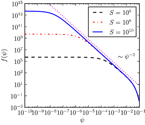
Figure 1: (Color online) The distribution function (2) for $S=10^{6}$, $10^{8}$, and $10^{10}$.

Under steady-state conditions, Eq. (1) admits the analytic solution

$$f(\psi)=\frac{2C/\alpha\tau_{A}}{\left(C-\exp(-\psi/\alpha\tau_{A})\right)^{2}}\exp(-\psi/\alpha\tau_{A}),$$ (2)

where the constant $C=1+2/n_{p}$ , with the total number of plasmoids $n_{p}=\int_{0}^{\infty}f(\psi)d\psi$. The source term $\zeta\delta(\psi)$ sets the boundary condition $f(0)=\zeta/\alpha$, which gives the relation $\zeta\tau_{A}=n_{p}^{2}/2+n_{p}.$ The source term magnitude $\zeta$ may be estimated by the relation $n_{p}\sim S/S_{c}$. In the limit $S\gg S_{c}$, we have $\zeta\sim n_{p}^{2}/2\tau_{A}\sim(S/S_{c})^{2}/2\tau_{A}$. The distribution function (2) has three distinct regimes when $S\gg S_{c}$ : (i) $f\simeq(2/\alpha\tau_{A})\exp(-\psi/\alpha\tau_{A})$ when $\psi/\alpha\tau_{A}\gg 1$; (ii) $f\simeq 2\alpha\tau_{A}\psi^{-2}$ when $2/n_{p}\ll\psi/\alpha\tau_{A}\ll 1$; (iii) $f\simeq n_{p}^{2}/2\alpha\tau_{A}$ when $\psi/\alpha\tau_{A}\ll 2/n_{p}$. Therefore, the solution admits both an exponential tail and a power-law regime. It can be shown that the dominant loss mechanism in the former regime is advection ($N\ll 1$;$\alpha\partial f/\partial\psi\simeq-f/\tau_{A}$), while it is coalescence in the latter ($N\gg 1$; $\alpha\partial f/\partial\psi\simeq-fN/\tau_{A}$). Figure 1 shows the distribution function (2) for $S=10^{6}$, $10^{8}$, and $10^{10}$. Here, to fix ideas, we have taken $S_{c}=10^{4}$, $V_{A}=1$, $B=1$, and $L=1$, and all scaling relations, such as $\alpha\sim BV_{A}/\sqrt{S_{c}}$, are replaced by equalities. Note that the range where the $f\sim\psi^{-2}$ power law holds is more extended for higher $S$.

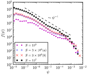
Figure 2: (Color online) Plasmoid distribution functions from direct numerical simulations.

To test the $f(\psi)\sim\psi^{-2}$ power law by DNS, we use the same simulation setup of two coalescing magnetic islands as in a previous study Huang and Bhattacharjee (2010). The 2D simulation box is the domain $(x,z)\in[-1/2,1/2]\times[-1/2,1/2]$. In normalized units, the initial magnetic field is given by $\mathbf{B}_{0}=\nabla\psi_{0}\times\mathbf{\hat{y}}$, where $\psi_{0}=\tanh\left(z/h\right)\cos\left(\pi x\right)\sin\left(2\pi z\right)/2\pi$. The parameter $h$, which is set to $0.01$ for all simulations, determines the initial current layer width. The initial plasma density $\rho$ is approximately $1$, and the plasma temperature $T$ is $3$. The density profile has a weak nonuniformity such that the initial condition is approximately force-balanced. The initial peak magnetic field and Alfvén speed are both approximately unity. The plasma beta $\beta\equiv p/B^{2}=2\rho T/B^{2}$ is greater than $6$ everywhere. Perfectly conducting and free slipping boundary conditions are imposed along both $x$ and $z$ directions. Only the upper half of the domain ($z\geq 0$) is simulated, and solutions in the lower half are inferred by symmetries. We use a uniform grid along the $x$ direction and a nonuniform grid along the $z$ direction that packs high resolution around $z=0$. For cases with $S=10^{6}$ and $3\times 10^{6}$, the mesh size is $12726\times 1600$, and the smallest grid size along $z$ is $5.7\times 10^{-6}$. For the $S=10^{7}$ case, the mesh size is $37800\times 2880$, and the smallest grid size along $z$ is $1.9\times 10^{-6}$. No explicit viscosity is employed in these simulations. A fourth order numerical dissipation is added to damp small fluctuations at grid scale Guzdar et al. (1993).

The initial velocity is seeded with a random noise of amplitude $10^{-6}$ to trigger the plasmoid instability. The early period when the reconnected flux is less than 0.01 is precluded from the analysis to allow the reconnection layer to reach a statistical steady state. We take data during the period when the reconnected flux is between $0.01$ to $0.05$, corresponding to $25\%$ of the initial flux in each of the merging islands. This period roughly spans $6\tau_{A}$, insensitive to $S$. Snapshots are taken at intervals of $0.01\tau_{A}$. We identify plasmoids within the range $x\in[-0.25,0.25]$ with a computer program for each snapshot, which provide the dataset for further statistical analysis. Figure 2 shows the probability distribution functions $f(\psi)$ for $S=10^{6}$, $3\times 10^{6}$ [two runs, labeled as (a) and (b)], and $S=10^{7}$. Distribution functions are normalized such that $\int_{0}^{\infty}f(\psi)d\psi$ is equal to the average number of plasmoids in each time slice. These numerical results appear to be robust and reproducible, as exemplified by the two $S=3\times 10^{6}$ runs that yield nearly identical distribution functions. Qualitative similarities between Fig. 1 and Fig. 2, especially the existence of three distinct regimes, are evident. However, the distribution function in the power-law regime is closer to $f(\psi)\sim\psi^{-1}$ instead of $f(\psi)\sim\psi^{-2}$.

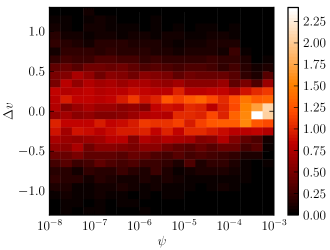
Figure 3: (Color online) The plasmoid distribution with respect to the relative speed $\mbox{$\Delta$}v$ and the flux $\psi$ from the run $S=10^{7}$.

To understand the discrepancy between the numerical results and the power-law prediction of Eq. (2), we need to critically examine the basic assumptions that give rise to the $f(\psi)\sim\psi^{-2}$ power law. In the $f(\psi)\sim\psi^{-2}$ regime, the dominant balance in Eq. (1) is between the plasmoid growth term and the loss term due to coalescence, i.e. $\alpha\partial f/\partial\psi\simeq-fN/\tau_{A}$. A key assumption underlying the loss term $-fN/\tau_{A}$ is that the relative speeds of a plasmoid with respect to neighboring plasmoids larger than itself are of the order of $V_{A}$ and are uncorrelated to the flux of the plasmoid. To examine this assumption with numerical data, we measure the relative velocity $\Delta v$ of each plasmoid at any given time with respect to the first larger plasmoid it will encounter by extrapolating the trajectories of the plasmoids with their velocities at that time. Note that $\Delta v$ is undefined for the largest plasmoid, or when all larger plasmoids are moving away from a given plasmoid. The plasmoids with $\Delta v$ undefined are disregarded in the analyses. Figure 3 shows the distribution $g(\psi,\Delta v)$ of plasmoids with respect to $\psi$ and $\Delta v$ from the run $S=10^{7}$. Here we normalize $g(\psi,\Delta v)$ such that $\int_{-\infty}^{\infty}g(\psi,\Delta v)d(\Delta v)=1$ for better visualization. We can clearly see that the distribution is not uniform across different values of $\psi$. The distribution covers a broader range of $\Delta v$ at smaller $\psi$, and it becomes more concentrated around $\Delta v=0$ at larger $\psi$. Similar results are also observed in other runs. Therefore, it appears that the reconnection layer organizes itself spontaneously into a state such that large plasmoids tend to avoid coalescing with each other.

How do we interpret this phenomenon? As discussed earlier, the flux of a plasmoid is approximately proportional to its age because all plasmoids grow approximately at the same rate $\alpha$. Consequently, a plasmoid can become large only if it has not encountered plasmoids larger than itself for an extended period of time. Presumably, plasmoids moving rapidly relative to their neighbors will encounter larger plasmoids and disappear easily, whereas those with small relative speeds are more likely to survive for a long time and become large. This observation motivates us to consider a distribution function $F(\psi,v)$, where $v$ can be interpreted as the plasmoid velocity relative to the mean flow (which has a profile along the outflow direction). The governing equation for $F(\psi,v)$ is written as

$$\partial_{t}F+\alpha\frac{\partial F}{\partial\psi}=\zeta\delta(\psi)h(v)-\frac{FH}{\tau_{A}}-\frac{F}{\tau_{A}},$$ (3)

where the function $H$ is defined as

$$H(\psi,v)=\int_{\psi}^{\infty}d\psi^{{}^{\prime}}\int_{-\infty}^{\infty}dv^{\prime}\frac{\left|v-v^{\prime}\right|}{V_{A}}F(\psi^{\prime},v^{\prime}),$$ (4)

and $h(v)$ is an arbitrary distribution function in velocity space when new plasmoids are generated. The distribution function $f(\psi)$ can be obtained by integrating $F(\psi,v)$ over the velocity space. Eq. (3) differs from Eq. (1) in the plasmoid loss term due to coalescence, where the relative speed $\left|v-v^{\prime}\right|$ between two plasmoids is taken into account in the integral operator of Eq. (4). If we replace $\left|v-v^{\prime}\right|$ in Eq. (4) by $V_{A}$, then Eq. (3) reduces to Eq. (1). Steady-state solutions of Eq. (3) can be obtained numerically. To fix ideas, we assume a Gaussian profile $h(v)=(1/\sqrt{\pi}V_{A})\exp(-v^{2}/V_{A}^{2})$ for the arbitrary source function. Fig. 4 shows the resulting $f(\psi)$ for $\zeta\tau_{A}=10^{6},$ $10^{7}$, and $10^{8}$. Assuming $n_{p}\simeq S/S_{c}$ and $S_{c}\simeq 10^{4}$, these solutions approximately correspond to $S=3\times 10^{7}$, $10^{8}$, and $3\times 10^{8}$, respectively. These solutions also show three distinct regimes as the solutions in Fig. 1. However, the distribution in the intermediate power-law regime is close to $f(\psi)\sim\psi^{-1}$, consistent with DNS. We have tried other smooth $h(v)$ profiles, and the results do not appear to be sensitive to the specific form of $h(v)$, as long as $h(v)$ covers a broad range of $v$ (typically of the order of $V_{A}$).

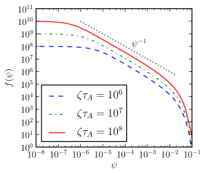
Figure 4: (Color online) Distribution functions from numerical solutions of Eq. (3).

A previous DNS study of plasmoid distribution has been recently carried out by Loureiro et al. Loureiro et al. (2012), where they claimed confirmation of the $f(\psi)\sim\psi^{-2}$ distribution. It should be pointed out that Loureiro et al. compared the $f(\psi)\sim\psi^{-2}$ prediction with simulation data in the large-$\psi$ regime. If we focus on the smaller-$\psi$ regime of their numerical data, the distribution appears more consistent with our finding $f(\psi)\sim\psi^{-1}$. This flattening of distribution function in the smaller-$\psi$ regime was noted by Loureiro et al., but no attempt was made to fit the smaller-$\psi$ regime to a power law. An important question is: do we expect to see a power law in the large-$\psi$ regime or the smaller-$\psi$ regime? Our analytic theory reveals that the transition from a power-law distribution to an exponential tail is due to a change in the dominant loss mechanism from coalescence to advection, which occurs approximately when $N\sim O(1)$. In our simulation data, the cumulative distribution function $N(\psi)$ drops below unity at $\psi\sim 10^{-3}$, which is also approximately where the distribution function deviates from $f(\psi)\sim\psi^{-1}$ to a more rapid, presumably exponential, falloff. Therefore, this rapidly falling tail is not where a power law should arise. However, simulation data in the large-$\psi$ regime is sufficiently uncertain that it may be difficult to make a clear distinction between a $\psi^{-2}$ and an exponential falloff. Note that the exponential falloff at large $\psi$ is consistent with the prediction of the kinetic model of Fermo et al. Fermo et al. (2010) and a subsequent analysis of the flux transfer events (FTEs) in the magnetopause from Cluster Fermo et al. (2011). Fermo et al. did not explicitly address the distribution of smaller plasmoids. Because the coalescence term in their model is based on very different considerations and assumptions, it is not clear whether the distribution of smaller plasmoids will follow a power law.

Although Eq. (3) is a significant improvement on Eq. (1), it does not include some important physical effects. Most notably, coalescence between islands is assumed to occur instantaneously, whereas in reality larger plasmoids take longer to merge, and there can be bouncing (or sloshing) between them Knoll and Chacón (2006); Karimabadi et al. (2011). These effects may also contribute to the distribution shown in Fig. 3. Furthermore, the velocity $v$ relative to the mean flow is assumed to remain constant throughout the lifetime of a plasmoid, whereas in reality some variation is expected due to the complex dynamics between plasmoids. Finally, in high-$S$ regime the current sheet between two coalescing plasmoids can also be the source of more plasmoids.Bárta et al. (2011).

It should be borne in mind that our considerations are valid for collisional plasmas obeying the resistive MHD equations. In weakly collisional systems the plasmoid instability inevitably drives reconnection towards the collisionless regime Daughton et al. (2009); Shepherd and Cassak (2010); Huang et al. (2011). The question of the plasmoid distribution in the collisionless regime remains largely open. However, some of the key ideas in this work, such as the tendency of large plasmoids to avoid coalescence, may still be relevant. The present study is limited to highly idealized 2D problems where more concrete conclusions can be drawn. In 3D geometry oblique tearing modes have been shown to play an important role Daughton et al. (2011); Baalrud et al. (2012), and a statistical description of such systems remains a great challenge.

This work was supported by the Department of Energy, Grant No. DE-FG02-07ER46372, under the auspice of the Center for Integrated Computation and Analysis of Reconnection and Turbulence (CICART), the National Science Foundation, Grant No. PHY-0215581 (PFC: Center for Magnetic Self-Organization in Laboratory and Astrophysical Plasmas), NASA Grant Nos. NNX09AJ86G and NNX10AC04G, and NSF Grant Nos. ATM-0802727, ATM-090315 and AGS-0962698. Computations were performed on Oak Ridge Leadership Computing Facility through an INCITE award, and National Energy Research Scientific Computing Center.

References

- Zweibel and Yamada (2009) E. G. Zweibel and M. Yamada, Annu. Rev. Astron. Astrophys. 47, 291 (2009).
- Biskamp (1986) D. Biskamp, Phys. Fluids 29, 1520 (1986).
- Lapenta (2008) G. Lapenta, Phys. Rev. Lett. 100, 235001 (2008).
- Bhattacharjee et al. (2009) A. Bhattacharjee, Y.-M. Huang, H. Yang, and B. Rogers, Phys. Plasmas 16, 112102 (2009).
- Cassak et al. (2009) P. A. Cassak, M. A. Shay, and J. F. Drake, Phys. Plasmas 16, 120702 (2009).
- Shepherd and Cassak (2010) L. S. Shepherd and P. A. Cassak, Phys. Rev. Lett. 105, 015004 (2010).
- Huang et al. (2011) Y.-M. Huang, A. Bhattacharjee, and B. P. Sullivan, Phys. Plasmas 18, 072109 (2011).
- Drake et al. (2006) J. F. Drake, M. Swisdak, H. Che, and M. A. Shay, Nature 443, 553 (2006).
- Daughton et al. (2006) W. Daughton, J. Scudder, and H. Karimabadi, Phys. Plasmas 13, 072101 (2006).
- Daughton et al. (2009) W. Daughton, V. Roytershteyn, B. J. Albright, H. Karimabadi, L. Yin, and K. J. Bowers, Phys. Rev. Lett. 103, 065004 (2009).
- Lin et al. (2008) J. Lin, S. R. Cranmer, and C. J. Farrugia, J. Geophys. Res. 113, A11107 (2008).
- Liu et al. (2010) R. Liu, J. Lee, T. Wang, G. Stenborg, C. Liu, and H. Wang, Astrophys. J. Lett. 723, L28 (2010).
- Nishizuka et al. (2010) N. Nishizuka, H. Takasaki, A. Asai, and K. Shibata, Astrophys. J. 711, 1062 (2010).
- Chen et al. (2008) L.-J. Chen, A. Bhattacharjee, P. A. Puhl-Quinn, H. Yang, N. Bessho, S. Imada, S. Muehlbachler, P. W. Daly, B. Lefebvre, Y. Khotyaintsev, A. Vaivads, A. Fazakerley, and E. Georgescu, Nature Physics 4, 19 (2008).
- Sweet (1958) P. A. Sweet, Nuovo Cimento Suppl. Ser. X 8, 188 (1958).
- Parker (1957) E. N. Parker, J. Geophys. Res. 62, 509 (1957).
- Loureiro et al. (2007) N. F. Loureiro, A. A. Schekochihin, and S. C. Cowley, Phys. Plasmas 14, 100703 (2007).
- Shibata and Tanuma (2001) K. Shibata and S. Tanuma, Earth Planets Space 53, 473 (2001).
- Huang and Bhattacharjee (2010) Y.-M. Huang and A. Bhattacharjee, Phys. Plasmas 17, 062104 (2010).
- Fermo et al. (2010) R. L. Fermo, J. F. Drake, and M. Swisdak, Phys. Plasmas 17, 010702 (2010).
- Uzdensky et al. (2010) D. A. Uzdensky, N. F. Loureiro, and A. A. Schekochihin, PRL 105, 235002 (2010).
- Fermo et al. (2011) R. L. Fermo, J. F. Drake, M. Swisdak, and K.-J. Hwang, J. Geophys. Res. 116, A09226 (2011).
- Loureiro et al. (2012) N. F. Loureiro, R. Samtaney, A. A. Schekochihin, and D. A. Uzdensky, Phys. Plasmas 19, 042303 (2012).
- Guzdar et al. (1993) P. N. Guzdar, J. F. Drake, D. McCarthy, A. B. Hassam, and C. S. Liu, Phys. Fluids B 5, 3712 (1993).
- Knoll and Chacón (2006) D. A. Knoll and L. Chacón, Phys. Plasmas 13, 032307 (2006).
- Karimabadi et al. (2011) H. Karimabadi, J. Dorelli, V. Roytershteyn, W. Daughton, and L. Chacón, PRL 107, 025002 (2011).
- Bárta et al. (2011) M. Bárta, J. Büchner, M. Karlický, and J. Skála, Astrophys. J. 737, 24 (2011).
- Daughton et al. (2011) W. Daughton, V. Roytershteyn, H. Karimabadi, L. Yin, B. J. Albright, B. Bergen, and K. J. Bower, Nature Physics 7, 539 (2011).
- Baalrud et al. (2012) S. D. Baalrud, A. Bhattacharjee, and Y.-M. Huang, Phys. Plasmas 19, 022101 (2012).