Low energy spectra in many flavor QCD with $N_{f}=$12 and 16

Abstract:

We present our result of the many-flavor QCD. Information of the phase structure of many-flavor SU(3) gauge theory is of great interest, since the gauge theories with the walking behavior near the infrared fixed point are candidates of new physics for the origin of the dynamical electroweak symmetry breaking. We study the SU(3) gauge theories with 12 and 16 fundamental fermions. Utilizing the HISQ type action which is useful to study the continuum physics, we analyze the lattice data of the mass and the decay constant of the pseudoscalar meson and the mass of the vector meson as well at several values of lattice spacing and fermion mass. The finite size scaling test in the conformal hypothesis is also performed. Our data is consistent with the conformal scenario for $N_{f}=12$. We obtain the mass anomalous dimension $\gamma_{m}\sim 0.4-0.5$. An update of $N_{f}=16$ study is also shown.

1 Introduction

There has been a renewed interest in the study of QCD with large number of the massless fermions in the fundamental representation (“large $N_{f}$ QCD”) in the context of walking technicolor having approximate scale invariance in the infrared (IR) region and large anomalous dimension $\gamma_{m}\simeq 1~{}$[1]. Such an approximate scale-invariant dynamics may in fact be realized in the large $N_{f}$ QCD: The perturbative two-loop beta function predicts a non-trivial infrared fixed point $\alpha_{*}$ ($0<\alpha_{*}<\infty$) in the range of $9\leq N_{f}\leq 16$ in the asymptotically free SU(3) gauge theory  [2, 3]. As a powerful tool of a nonperturbative study, one uses lattice QCD simulations, which can in principle determine the phase structure of the SU(3) gauge theories with various number of fermions. In addition to the pioneering works [4, 5, 6], there are many lattice works in the large $N_{f}$ QCD in the recent years. In particular, the system of the $N_{f}=12$ has been widely investigated by the lattice approach, such as running coupling, lattice phase diagram, low-energy spectra and so on. (See, for a review, Ref. [7].)

We investigate the 12 and 16-flavor SU(3) gauge theories using a variant of the highly improved staggered quark (HISQ) action [8] to reduce the discretization error. We study several bound-state masses such as the pseudoscalar meson $\pi$ and vector meson $\rho$ as well as the decay constant of $\pi$, by varying the fermion bare mass $m_{f}$. In this work, we introduce a quantity for the scaling test of the conformal hypothesis with finite volume in the analyses for $N_{f}=12$. Using this quantity, we can analyze the data without any assumption of the fitting form in the scaling test. We also discuss possible finite size and mass corrections in the scaling. We find that our results of $N_{f}=12$ are consistent with hyperscaling with $\gamma=0.4-0.5$. These results of $N_{f}=12$ have already been published in Ref. [9].

Besides the $N_{f}=12$ theory, we also simulate the $N_{f}=16$ theory with the same setup. Since this theory is expected to deeply reside in the conformal phase, it is helpful to understand conformal signals from numerical simulations. The preliminary results of this theory are also shown.

2 $N_{f}=12$

We use a version of the HISQ [8] action for many-flavor simulations but without the tadpole improvement and the mass correction term for heavy fermions. Gauge configurations are generated by HMC algorithm using MILC code ver.7 with various parameter sets for the fermion mass $m_{f}$, volume and the bare coupling $\beta=6/g^{2}$. We calculate several bound-state masses, such as the pseudoscalar meson $\pi$ and vector meson $\rho$, and the decay constant of $\pi$. If the theory is in the conformal window, the hadron mass $M_{H}$ and $\pi$ decay constant $F_{\pi}$ obey the conformal hyperscaling

$$M_{H}\propto m_{f}^{\frac{1}{\gamma_{*}+1}},\;F_{\pi}\propto m_{f}^{\frac{1}{\gamma_{*}+1}},$$ (1)

where $\gamma_{*}$ denotes the mass anomalous dimension at the IR fixed point. On the other hand, if the theory is in the phase of chiral symmetry breaking, the leading fermion mass dependence of $\pi$ is

$$M_{\pi}^{2}\propto m_{f},\;F_{\pi}=c_{0}+c_{1}m_{f},$$ (2)

with $c_{0}\neq 0$, and the vector meson mass does not vanish in the chiral limit.

The spectra obtained in our lattice simulation will be tested against these two hypotheses in this work.

2.1 Primary analysis

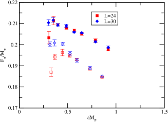
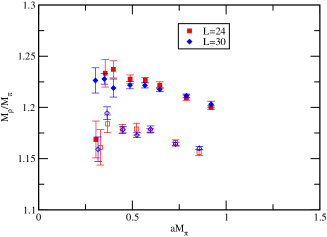
For a primary analysis dimensionless ratios, $F_{\pi}/M_{\pi}$ and $M_{\rho}/M_{\pi}$, are plotted against $aM_{\pi}$ in Fig. 1. The left panel plots $F_{\pi}/M_{\pi}$ on the largest two volumes at the two bare gauge couplings $\beta=3.7$ and $4$. If we look at the results for $\beta=3.7$ (filled symbols), $F_{\pi}/M_{\pi}$ tends to be flat for smaller $\pi$ masses, which shows clear contrast to ordinary QCD case. The behavior is consistent with the hyperscaling in Eq. (1). The $M_{\pi}$ dependence of the ratio at the larger mass can be realized by the correction to the hyperscaling which may be different from one quantity to another. For $\beta=4$ (open symbols) there is no flat range without volume dependence. Similar observation can be made for the other ratio $M_{\rho}/M_{\pi}$ shown in the right panel of Fig. 1. The flattening is observed for $\beta=3.7$ again, but the range is wider than $F_{\pi}/M_{\pi}$. In this case $\beta=4$ shows the flattening, too. The difference of the constant in the flat region could be caused by a discretization effect.

Existence of the scaling for $F_{\pi}$ at $\beta=3.7$ and absence at $\beta=4$ at the same $aM_{\pi}$ can be made possible if the $M_{\pi}$ in the physical unit is larger (thus the correction is no longer negligible) for $\beta=4$, i.e., the lattice spacing decreases as $\beta$ increases. In that case the physical volume is smaller for $\beta=4$, which gives a reason for the volume effect observed only for $\beta=4$. Actually a crude analysis of two lattice spacing matching shows the result $a(\beta=3.7)>a(\beta=4)$ which is consistent with being in the asymptotically free domain.

Figure 1: Dimension-less ratios $F_{\pi}/M_{\pi}$ and $M_{\rho}/M_{\pi}$ as functions of $aM_{\pi}$ for $N_{f}=12$ at $\beta=3.7$ (filled symbol) and $4.0$ (open symbol) for two largest volumes.

2.2 Finite-size hyperscaling

In the conformal window with finite masses and volume, the renormalization group analysis tells us that the scaling behavior for low-energy spectra which should obey the universal scaling relations  as

$$\xi_{p}\equiv LM_{p}=f_{p}(x),\quad\xi_{F}\equiv LF_{\pi}=f_{F}(x),$$ (3)

where the subscript $p$ distinguishes the bound state, $p=\pi$ or $\rho$ in this study. The product of bound state mass or decay constant and linear system size falls into a function of a single scaling variable $x=L\cdot m_{f}^{\frac{1}{1+\gamma_{*}}}$, where $\gamma_{*}$ is the mass anomalous dimension at the IR fixed point. We shall call the scaling relation the finite-size hyperscaling (FSHS). While the forms of the scaling functions $f_{p}(x)$ are unknown in general, the asymptotic form should be $f(x)\sim x$ at large $x$ because it must reproduce the hyperscaling relation Eq. (1) in large volumes.

Now we examine whether our data for the bound state masses and decay constant obey FSHS. To visualize how the scaling works we show $\xi_{\pi}$ as functions of $x=L\cdot m_{f}^{1/(1+\gamma)}$ for several values of $\gamma$ in Fig. 2. It is observed that the data align well with around $\gamma=0.4$, while they become scattered for $\gamma$ away from that value. This indicates the existence of possible FSHS with $\gamma\sim 0.4$.

Figure 2: $\xi_{\pi}$ is plotted as a function of the scaling variable $x$ for $\gamma=0.1$, $0.4$, and $0.7$ from left to right for $N_{f}=12$ at $\beta=3.7$. An alignment is seen for $\gamma\sim 0.4$.

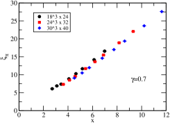
A similar alignment is observed for $\xi_{F}$ as well. In this case one finds the optimal scaling at around $\gamma\sim 0.5$.

To quantify the “alignment” we introduce an evaluation function $P(\gamma)$ for an observable $p$ as follows. Suppose $\xi^{j}$ be a data point of the measured observable $p$ at $x_{j}=L_{j}\cdot m_{j}^{1/(1+\gamma)}$ and $\delta\xi^{j}$ be the error of $\xi^{j}$. $j$ labels distinction of parameters $L$ and $m_{f}$. Let $K$ be a subset of data points $\{(x_{k},\xi_{k})\}$ from which we construct a function $f^{(K)}(x)$ that represents the subset of data. Then the evaluation function is defined as

$$P(\gamma)=\frac{1}{\mathcal{N}}\sum_{L}\sum_{j\not\in{K_{L}}}\frac{\left|\xi^{j}-f^{(K_{L})}(x_{j})\right|^{2}}{\left|\delta\xi^{j}\right|^{2}},$$ (4)

where $L$ runs through the lattice sizes we have, the sum over $j$ is taken for a set of data points that do not belong to $K_{L}$ which includes all the data obtained on the lattice with size $L$. $\mathcal{N}$ denotes the total number of summation. Here we choose for the function $f^{(K_{L})}$ a linear interpolation of the data points of the fixed lattice size $L$ for simplicity, which should be a good approximation of $\xi$ for large $x$. In the evaluation function Eq. (4), the data points need to be taken for a range of $x=L\cdot m_{f}^{1/(1+\gamma)}$ in which there is an overlap of available data for all volumes, $L=18$, $24$, and $30$ within the range $[x_{\text{min}},x_{\text{max}}]$. We take the value of $x_{\text{min}}$ ($x_{\text{max}}$) as the smallest (largest) $m_{f}$ for the largest (smallest) volume $L$ in our simulation parameters. Note, however, we may need to incorporate some neighboring data outside this range to obtain the interpolated value $f^{(K)}(x)$ by the spline functions.

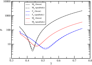
The evaluation function for all the quantities, $M_{\pi}$, $M_{\rho}$ and $F_{\pi}$, is plotted in the left panel of Fig. 3. A clear minimum is observed at which the optimal alignment of the data is achieved. It is noted that the value of $P(\gamma)$ is $\mathcal{O}(1)$ at the minimum. The systematic error due to the ambiguity of the interpolation is estimated by the difference of the optimal $\gamma$’s obtained with linear and quadratic spline interpolations. The comparison of these $P(\gamma)$’s is also shown in the left panel of Fig. 3. The minima for the quadratic spline interpolation appear approximately at the same place as those for the linear one. It is found that this systematic error is always smaller than the statistical error. The other uncertainties due to the finite size and mass effects are estimated by the variations of optimal $\gamma$ with respect to the change of both the x-range and $L$ used in the analyses. The results with all the errors added in quadrature are summarised in the right panel of Fig. 3. The details of the analysis are shown in Ref. [9].

Figure 3: (Left) The $\gamma$ dependence of the evaluation function $P$ for $M_{\pi}$, $F_{\pi}$, and $M_{\rho}$ at $\beta=3.7$ is plotted. The vertical axis shows the values of $P$ at each of $\gamma$ where the three volumes and full range of $x$ for the data are considered. The solid and dashed curves show the results of $P(\gamma)$ with the interpolation functions $f(x)$ by the linear and quadratic functions, respectively. (Right) The results of the values of $\gamma$ for three observables at two $\beta$ are summarized, where the statistical and systematic errors are added in quadrature.

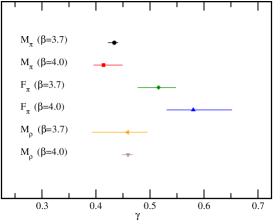
All the results are consistent with each other within $2\sigma$ level, except for $\gamma$ from $F_{\pi}$ at $\beta=4$ for which the scaling region was suspected to be outside of the parameter range we have examined in the previous subsection. From these analyses, we conclude that our data for the $N_{f}=12$ theory are reasonably consistent with the FSHS. The resulting mass anomalous dimensions is $0.4\leq\gamma_{*}\leq 0.5$.

In the test of the chiral broken scenario, it turns out that the natural chiral expansion parameter $\chi=N_{f}\left(\frac{M_{\pi}}{4\pi F_{\pi}/\sqrt{2}}\right)^{2}$ is very large in the region we simulated, which is evaluated as $\chi\sim 39$ at the smallest $M_{\pi}$ using the value of $F_{\pi}$ in the chiral limit. With this large $\chi$, we could not consistently analyze the data based on the ChPT. Further efforts would be required to arrive at a decisive conclusion.

3 $N_{f}=16$

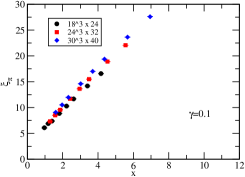
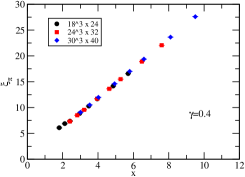
In the previous report [12] we presented that the result of the $\xi_{\pi}$ is consistent with the FSHS, but the optimal $\gamma$ decreases as $\beta$ increases in $\beta\leq 3.5$. Furthermore the results of the $\gamma$ is much larger than the perturbative result, $\gamma\sim 0.025$. In this theory the perturbation would be reliable because of the small coupling constant at the IR fixed point, so that we considered that our result contains large systematic errors. Thus, we investigate the $\beta$ dependence of $\gamma$ in larger $\beta$ region than the ones we simulated in the previous report.

Using the same simulation setup as in $N_{f}=12$, we perform simulations at several values of $\beta$ adding to the previous work, such as 5 and 12, on various spatial volumes, $L=8,12,16,24$ and 30. The range of the fermion mass is $0.03\leq m_{f}\leq 0.2$, and the typical length of the trajectory is roughly 1000.

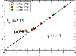
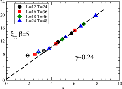
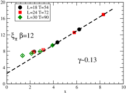
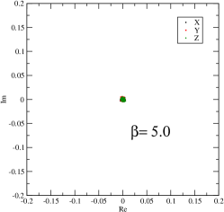
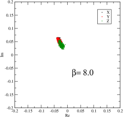
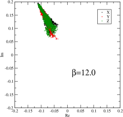
The plots in Fig. 4 show that for $\beta=5$ and 12 the $\xi_{\pi}$ aligns well as a function of $x$ using an optimal value of the $\gamma$ as in the $N_{f}=12$ case. The value, however, largely depends on $\beta$. At the highest $\beta$ the $\gamma$ is still five times larger than the perturbative result, although the result at this $\beta$ would include large systematic error coming from finite volume. Fig. 5 shows the scatter plots of Polyakov loop in the spatial directions with fixed bare mass $m_{f}=0.3$ and lattice sizes $L=18,T=32$. As shown here, at the highest $\beta$, the Polyakov loop has a non-zero value associated with the center symmetry breaking. On the other hand, at the lower $\beta$ region, this value decreases with $\beta$. We consider that this symmetry breaking at the higher $\beta$ occurs due to the small physical volume, so that to reduce finite volume effects we would need much larger lattice size than $L=18$ at $\beta=12$. We will continue investigations with larger volumes at higher $\beta$ region to obtain the correct value of the $\gamma$ at the vicinity of the infrared fixed point.

Figure 4: $\xi_{\pi}$ in the 16 flavors at $\beta=3.15$(left), 5(center) and $12$(right). The different symbols denote the data at the different volumes. The dashed line denotes the fit result of the finite-size hyperscaling. The filled and open symbols represent the data included in the fit and omitted from the fit, respectively.

Figure 5: Scatter plot of the Polyakov loops in the spacial directions.

4 Summary and outlook

We have studied the SU(3) gauge theories with the fundamental 12 and 16 fermions using a HISQ type staggered fermion action, For the 12-flavor case, we attempt to determine the phase of this theory through the analysis of $M_{\pi}$, $M_{\rho}$ and $F_{\pi}$. Our present data is consistent with the conformal hypothesis. The mass anomalous dimension, $\gamma_{*}$ at the infrared fixed point was estimated through the (finite-size) hyperscaling analysis. Our result is $\gamma_{*}\sim 0.4-0.5$, which is not as big as $\gamma_{*}\sim 1$ for the theory to be close to the realistic technicolor model. In the test of chiral broken scenario, the chiral expansion parameter $\chi$ is much larger than one even at the smallest $M_{\pi}$. We could not consistently analyze the data based on the chiral expansion. A possibility of the chiral broken phase in $N_{f}=12$ is not excluded yet. More detailed analyses with more data at larger volume and lighter mass would be required. For the 16-flavor case, the pion mass data exhibit the scaling which is consistent with the conformal scenario, while the obtained value of the $\gamma$ is much bigger than the perturbative result. To obtain the $\gamma$ at the infrared fixed point, further study of the $\gamma$, especially volume dependence would be required. Another series of the study in our project has been reported for the test of the walking behavior in $N_{f}=8$ [13], and an analytical calculation of the hyperscaling through the Schwinger-Dyson equation [14].

References

- [1] K. Yamawaki, M. Bando and K. -i. Matumoto, Phys. Rev. Lett. 56, 1335 (1986).
- [2] W. E. Caswell, Phys. Rev. Lett. 33 (1974) 244.
- [3] T. Banks and A. Zaks, Nucl. Phys. B 196 (1982) 189.
- [4] Y. Iwasaki, K. Kanaya, S. Sakai and T. Yoshie, Phys. Rev. Lett. 69 (1992) 21.
- [5] F. R. Brown, H. Chen, N. H. Christ, Z. Dong, R. D. Mawhinney, W. Schaffer and A. Vaccarino, Phys. Rev. D 46 (1992) 5655 [hep-lat/9206001].
- [6] P. H. Damgaard, U. M. Heller, A. Krasnitz and P. Olesen, Phys. Lett. B 400 (1997) 169 [hep-lat/9701008].
- [7] J. Giedt, plenary talk at Lattice 2012, PoS LATTICE 2012 (2012) 006; E. T. Neil, PoS LATTICE 2011, 009 (2011) [arXiv:1205.4706 [hep-lat]], and references therein.
- [8] E. Follana et al. [HPQCD and UKQCD Collaborations], Phys. Rev. D 75 (2007) 054502 [hep-lat/0610092].
- [9] Y. Aoki, T. Aoyama, M. Kurachi, T. Maskawa, K. -i. Nagai, H. Ohki, A. Shibata, K. Yamawaki, T. Yamazaki, (LatKMI collaboration), Phys. Rev. D 86 (2012) 054506 [arXiv:1207.3060 [hep-lat]].
- [10] T. DeGrand and A. Hasenfratz, Phys. Rev. D 80 (2009) 034506 [arXiv:0906.1976 [hep-lat]].
- [11] L. Del Debbio and R. Zwicky, Phys. Rev. D 82 (2010) 014502 [arXiv:1005.2371 [hep-ph]].
- [12] Y. Aoki, T. Aoyama, M. Kurachi, T. Maskawa, K. -i. Nagai, H. Ohki, A. Shibata, K. Yamawaki, T. Yamazaki, (LatKMI collaboration), PoS LATTICE 2011, 080 (2011) [arXiv:1202.4712 [hep-lat]].
- [13] Y. Aoki, T. Aoyama, M. Kurachi, T. Maskawa, K. -i. Nagai, H. Ohki, A. Shibata, K. Yamawaki, T. Yamazaki, (LatKMI collaboration), talk at Lattice 2012, PoS LATTICE 2012 (2012) 035.
- [14] Y. Aoki, T. Aoyama, M. Kurachi, T. Maskawa, K. -i. Nagai, H. Ohki, A. Shibata, K. Yamawaki, T. Yamazaki, (LatKMI collaboration), Phys. Rev. D 85 (2012) 074502 [arXiv:1201.4157 [hep-lat]]; talk at Lattice 2012, PoS LATTICE 2012 (2012) 059.