Correlation enhanced phase sensitive Raman scattering in atomic vapors

Abstract

We theoretically propose a method to enhance Raman scattering by injecting a seeded light field which is correlated with the initially prepared atomic spin wave. Such a light-atom correlation leads to an interference in the Raman scattering. The interference is sensitive to the relative phase between the seeded light field and initially prepared atomic spin wave. For constructive interference, the Raman scattering is greatly enhanced. Such an enhanced Raman scattering may find applications in quantum information, nonlinear optics and optical metrology due to its simplicity.

I Introduction

The cooperative spontaneous emission of radiation (superradiance) from an ensemble was first introduced by Dicke in 1954 Dicke , where an atomic ensemble exhibited enhanced coupling to a single electromagnetic mode. Superradiance was initially suggested for sample dimensions $R$ much smaller than the wavelength $\lambda$ of the resonant transition Dicke . However, the case in the opposite limit $R\gg\lambda$ has also attracted extensive research Smithey ; Jain ; Black ; Simon07 ; Simon ; Scully09 ; Sete ; Chen09 ; Chen10 ; Agarwal11 because in quantum optics the sample is usually large compared to $\lambda$. In such a large-size sample, the superradiance is difficult to happen according to the standard argument that the dipole-dipole interaction between atoms is too weak to build a macroscopic dipole moment. To have enhancement in the limit of large-size sample with $R\gg\lambda$, the quantum coherence and interference must enter to play a role. Typical example is to employ the quantum coherence to enhance some nonlinear optical processes Lukin ; Boyd . Recently, our group observed an enhanced Raman scattering effect by using an atomic spin wave, a coherence prepared between atomic ground-state sublevels Chen09 ; Chen10 . The subsequent theoretical analysis modeled the experiment where an early spontaneous Raman scattering (SRS) generated the atomic spin wave which causes enhancement of the Raman light fields in the second Raman scattering Yuan10 . The flipped atoms act as seeds to the second Raman process which amplifies the light fields all the way through the atomic ensembles.

In this paper, based on our previous work Chen09 ; Chen10 ; Yuan10 , we propose a scheme to enhance the Raman scattering, termed as correlation-enhanced Raman scattering (CERS). In the scheme, a pump field leads to spontaneous emission of the Stokes field, accompanying with the generation of atomic spin waves. Then this Stokes field used as a seeded signal, with the pump field together, is subsequently input into atomic ensemble to generate a second Stokes field. A CERS occurs due to the correlation of the seeding Stokes field and atomic spin waves Smithey ; Raymer04 ; Wasilewski ; Ji07 ; Bian . Such a light-atom correlation is a new mechanism to enhance Raman scattering, which is different from the idea of the so-called super Raman scattering initiated by the atom-atom entangled state Agarwal11 .

Our article is organized as follows. In Sec. II, the general model involving spatial propagation and light-atom coupling in Raman scattering is reviewed. The correlation of the light field and the atomic spin wave is derived from the light-atom coupling equations. Based on the model, the CERS is studied in detail in Sec. III. In Sec. IV, we numerically calculate the intensity of CERS based on the correlation of the seeded field and the atomic spin wave. Finally, we conclude with a summary of our results.

II Light-atom Correlation in Raman Scattering

In this section, we give a brief review of the theoretical model of Raman scattering. The Raman scattering process in atomic system is described through a three-level model [see Fig.1(a)] coupled to a pump field and a Stokes field. For convenience, assume the pump field corresponding to a focused beam and the Fresnel number $\mathfrak{F}=A/\lambda_{S}L$ ($A$ cross-sectional area, $L$ cell length) is of the order of unity, then only a single transverse spatial mode contributes strongly to emission along the direction of propagation the pump field. Therefore, a simplified one-dimensional model can be enough to describe the Raman scattering. In the case of large light detuning, the atomic excited state can adiabatically be eliminated and one obtains the light-atom coupling equations governing the propagation of the quantized Stokes field and the atomic ground-state spin excitations determined by the spin wave Yuan10 ; Raymer81

$$(\partial_{t}+c\partial_{z})\hat{\mathcal{E}}_{S}(z,t)=i\chi\hat{S}_{a}^{{\dagger}},$$ (1)

$$\partial_{t}\hat{S}_{a}^{{\dagger}}(z,t) =-\Gamma_{S}\hat{S}_{a}^{{\dagger}}-i\mathcal{W}\chi^{\ast}\hat{\mathcal{E}}_{S}+\hat{F}_{S}^{\dagger},$$ (2)

$$\partial_{t}\mathcal{W}(z,t) =-\gamma_{L}\mathcal{W}-\gamma_{L},$$ (3)

where $\hat{S}_{a}=\sqrt{N}\tilde{\sigma}_{12}e^{-i\Delta kz}$ the spin wave operator, $N$ the number of atoms, $\Delta k=k_{P}-k_{S}$, $\tilde{\sigma}_{\mu\nu}(z,t)=1/N_{z}\sum_{j=1}^{N_{z}}\hat{\sigma}_{\mu\nu}^{j}$ the collective atomic operators, where $\hat{\sigma}_{\mu\nu}^{j}=|\mu\rangle_{jj}\langle\nu|$ ($\mu,\nu=1,2$) is the transition operator of the $j$th atom between states $|\mu\rangle$ and $|\nu\rangle$ and a small and macroscopic volume containing $N_{z}$ $(N_{z}\gg 1)$ atoms around position $z$, and the commutation relation is $[\tilde{\sigma}_{\mu\nu}(z,t),\tilde{\sigma}_{\alpha\beta}(z^{\prime},t)]=L/N\delta(z-z^{\prime})(\delta_{\nu\alpha}\tilde{\sigma}_{\mu\beta}(z,t)-\delta_{\mu\beta}\tilde{\sigma}_{\alpha\nu}(z,t))$, $L$ the length of the atomic medium. $\hat{\mathcal{E}}_{S}(z,t)$ is a slowly varying envelope operator of the Stokes field $\hat{E}_{S}^{(+)}=\sqrt{\hbar\omega/2\varepsilon_{0}AL}\hat{\mathcal{E}}_{S}(z,t)e^{i(\mathbf{k}_{S}\cdot\mathbf{z}-\omega_{S}t)}$, and $A$ is cross-section area, and its commutation relation $[\hat{\mathcal{E}}_{S}(z,t),\hat{\mathcal{E}}_{S}(z,t^{\prime})]=L/c\delta(t-t^{\prime})$.$\ \chi(z,t)=g\sqrt{N}\Omega_{P}(z,t)/\Delta$ the coupling coefficient between spin excitations and stokes field, $\Omega_{P}(z,t)$ the Rabi frequency of pump field, $g$ the atom-field coupling constant, $\Gamma_{S}=\gamma_{S}-i\delta_{L}$, $\gamma_{S}=\gamma_{S_{0}}+\gamma_{L}$, and $\gamma_{L}=\gamma|\Omega_{P}|^{2}/\Delta^{2}$ is the optical pumping rate, and $\delta_{L}=|\Omega_{P}|^{2}/\Delta$ is the ac Stark shift, and $\gamma_{S_{0}}$ the coherence ($\tilde{\sigma}_{12}$) decay rate, $\gamma$ the decay rates of the excited state $|3\rangle$ to states $|1\rangle$ and $|2\rangle$ (assuming $\gamma_{31}=\gamma_{32}=\gamma$). $\mathcal{W}(z,t)=\tilde{\sigma}_{11}(z,t)-\tilde{\sigma}_{22}(z,t)$ describes the population difference between energy levels $|1\rangle$ and $|2\rangle$. In general, $\mathcal{W}(z,t)$ is related to the collective atomic excitation number and the strength of atomic coherence. Here we consider weak excitations, and $\mathcal{W}(z,t)$ is approximately determined by Eq. (3). The Langevin noise operator $\hat{F}_{S}^{\dagger}$ has the correlation $\langle\hat{F}_{S}(z,t)\hat{F}_{S}^{\dagger}(z^{\prime},t^{\prime})\rangle=2\gamma_{S}L\delta(z-z^{\prime})\delta(t-t^{\prime})$.

For convenience in analysis, neglecting the depletion of the pump field by making $\Omega_{P1,2}(z,t)\equiv\Omega_{P1,2}(t)=\Omega_{P1,2}\theta(t)$ with $\Omega_{P1,2}$ being constant and $\theta(t)$ the step function. Similarly, $\chi(z,t)\equiv\chi(t)=g\sqrt{N}\Omega_{P}(t)/\Delta$. Using the moving coordinates $t^{\prime}=t-z/c$, $z^{\prime}=z$, the solutions of Eqs. (1)-(3) are given for the Raman scattering Yuan10 ; Raymer81 ,

$$\hat{\mathcal{E}}_{S}(z^{\prime},t^{\prime})=\mathcal{U}_{S}(z^{\prime},t^{\prime})\{\hat{\mathcal{E}}_{S}(0,t^{\prime\prime})\}+\mathcal{V}_{S}(z^{\prime},t^{\prime})\{\hat{S}_{a}^{\dagger}(z^{\prime\prime},0)\}$$

$$\text{ \ \ \ \ \ \ \ \ \ \ \ \ \ \ \ \ \ \ \ \ \ \ }+\mathcal{F}_{S}(z^{\prime},t^{\prime})\{\hat{F}_{S}^{\dagger}(z^{\prime\prime},t^{\prime\prime})\},$$ (4)

$$\hat{S}_{a}^{{\dagger}}(z^{\prime},t^{\prime})=\mathcal{U}_{a}(z^{\prime},t^{\prime})\{\hat{S}_{a}^{\dagger}(z^{\prime\prime},0)\}+\mathcal{V}_{a}(z^{\prime},t^{\prime})\{\hat{\mathcal{E}}_{S}(0,t^{\prime\prime})\}$$

$$\text{ \ \ \ \ \ \ \ \ \ \ \ \ \ \ \ \ \ \ \ \ \ \ }+\mathcal{F}_{a}(z^{\prime},t^{\prime})\{\hat{F}_{S}^{\dagger}(z^{\prime\prime},t^{\prime\prime})\},$$ (5)

$$\mathcal{W}(t^{\prime})=\mathcal{W}(0)e^{-\Gamma_{L}(t^{\prime})}-\int_{0}^{t^{\prime}}\gamma_{L}(t^{\prime\prime})e^{-[\Gamma_{L}(t^{\prime})-\Gamma_{L}(t^{\prime\prime})]}dt^{\prime\prime},$$

where

$$\mathcal{U}_{S}(z^{\prime},t^{\prime})\{...\}=\int_{0}^{t^{\prime}}dt^{\prime\prime}[2\delta(t^{\prime}-t^{\prime\prime})+\chi(t^{\prime})\chi^{\ast}(t^{\prime\prime})$$

$$~{}~{}\text{\ \ \ \ \ \ \ \ \ }\times e^{-[\Gamma(t^{\prime})-\Gamma(t^{\prime\prime})]}\frac{\mathcal{W}(t^{\prime\prime})}{c}G_{e}(z^{\prime},0,t^{\prime},t^{\prime\prime})]\{...\},$$

$$\mathcal{V}_{S}(z^{\prime},t^{\prime})\{...\}=i\int_{0}^{z^{\prime}}dz^{\prime\prime}\frac{\chi(t^{\prime})}{c}e^{-\Gamma(t^{\prime})}H(z^{\prime},z^{\prime\prime},t^{\prime},0)\{...\},$$

$$\mathcal{U}_{a}(z^{\prime},t^{\prime})\{...\}=\int_{0}^{z^{\prime}}dz^{\prime\prime}e^{-\Gamma(t^{\prime})}[2\delta(z^{\prime}-z^{\prime\prime})$$

$$\text{ \ \ \ \ \ \ \ \ \ \ }\times G_{S}(z^{\prime},z^{\prime\prime},t^{\prime},0)]\{...\},$$

$$\mathcal{V}_{a}(z^{\prime},t^{\prime})\{...\}=-i\int_{0}^{t^{\prime}}dt^{\prime\prime}\mathcal{W}(t^{\prime\prime})\chi^{\ast}(t^{\prime\prime})e^{-[\Gamma(t^{\prime})-\Gamma(t^{\prime\prime})]}$$

$$\text{ \ \ \ \ \ \ \ \ \ \ }\times H(z^{\prime},0,t^{\prime},t^{\prime\prime})\{...\},$$

$$\mathcal{F}_{S}(z^{\prime},t^{\prime})\{...\}=i\int_{0}^{t^{\prime}}dt^{\prime\prime}\int_{0}^{z^{\prime}}dz^{\prime\prime}\frac{\chi(t^{\prime})}{c}e^{-[\Gamma(t^{\prime})-\Gamma(t^{\prime\prime})]}$$

$$\text{ \ \ \ \ \ \ \ \ \ \ }\times H(z^{\prime},z^{\prime\prime},t^{\prime},t^{\prime\prime})\{...\},$$

$$\mathcal{F}_{a}(z^{\prime},t^{\prime})\{...\}=\int_{0}^{t^{\prime}}dt^{\prime\prime}\int_{0}^{z^{\prime}}dz^{\prime\prime}e^{-[\Gamma(t^{\prime})-\Gamma(t^{\prime\prime})]}$$

$$\text{ \ \ \ \ \ \ \ \ \ \ }\times[2\delta(z^{\prime}-z^{\prime\prime})+G_{S}(z^{\prime},z^{\prime\prime},t^{\prime},t^{\prime\prime})]\{...\},$$ (7)

in which

$$H(z^{\prime},z^{\prime\prime},t^{\prime},t^{\prime\prime})=I_{0}(2\sqrt{[q(t^{\prime})-q(t^{\prime\prime})]\frac{z^{\prime}-z^{\prime\prime}}{c}}),$$

$$G_{e}(z^{\prime},z^{\prime\prime},t^{\prime},t^{\prime\prime})=\frac{c(z^{\prime}-z^{\prime\prime})}{q(t^{\prime})-q(t^{\prime\prime})}G_{S}(z^{\prime},z^{\prime\prime},t^{\prime},t^{\prime\prime}),$$

$$G_{S}(z^{\prime},z^{\prime\prime},t^{\prime},t^{\prime\prime})=\sqrt{\frac{q(t^{\prime})-q(t^{\prime\prime})}{c(z^{\prime}-z^{\prime\prime})}}$$

$$\times I_{1}(2\sqrt{[q(t^{\prime})-q(t^{\prime\prime})]\frac{z^{\prime}-z^{\prime\prime}}{c}}).$$ (8)

Here $q(t^{\prime})=\int_{0}^{t^{\prime}}\mathcal{W}(t^{\prime\prime})\chi(t^{\prime\prime})^{2}dt^{\prime\prime}$, $\Gamma(t^{\prime})=\int_{0}^{t^{\prime}}\Gamma_{S}(t^{\prime\prime})dt^{\prime\prime}$, $\Gamma_{L}(t^{\prime})=\int_{0}^{t^{\prime}}\gamma_{L}(t^{\prime\prime})dt^{\prime\prime}$, and $I_{n}(x)$ is the modified Bessel function of the first kind of order $n$.

The integral solutions presented in Eqs. (4)-(5) indicate that the Stokes field $\hat{\mathcal{E}}_{S}(z^{\prime},t^{\prime})$ contains three parts of contributions, the first one from the input field plus the scattering field, the second from the initial spin excitations, and the third from the atomic fluctuations. Similarly, the generated spin wave $\hat{S}_{a}^{\dagger}(z^{\prime},t^{\prime})$ contains the contributions from the initial spin excitations, the input field, and the atomic fluctuations. Evidently a light-atom correlation of the Stokes field and the generated spin wave, $\hat{\langle\mathcal{E}}_{S}(z,t^{\prime})\hat{S}_{a}(z^{\prime},t^{\prime})\rangle\neq 0,$ is built through the Raman coupling as seen in Eqs. (4)-(5).

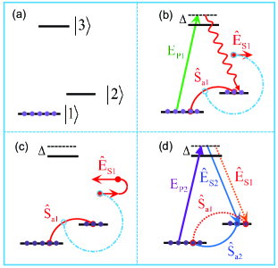
Figure 1: (Color online) (a) Initially prepared ground state for SRS. (b) SRS process: a Stokes field and its correlated atomic spin wave are generated. The light-atom correlation is denoted by the circular arc (dotted-dashed blue line). (c) The light field and its correlated atomic spin wave, generated in the SRS process, are used as initial seeding for CERS. (d) CERS process: an enhanced Stokes field $\hat{E}_{S{2}}$ is generated by the pump $E_{P{2}}$ with the initial seeding state (c). $E_{P{1,2}}$: pump fields; $\hat{E}_{S{1,2}}$ and $\hat{S}_{a{1,2}}$: the generated Stokes fields and spin waves, respectively; $\Delta$: the detuning.

III Correlation-enhanced Raman Scattering

In the section, we study the role of the correlation of the light field and atomic spin wave in enhancing Raman scattering. The basic idea is as follows. First we employ a SRS process to generate a light field and an atomic spin wave which are correlated with each other. The SRS process is illustrated in Figs. 1(a) and (b), where an atomic ensemble, initially prepared in the ground state, is pumped by an off-resonance pump field $E_{P1}$ and spontaneously emitted a Stokes field $\hat{E}_{S1}$. As a result, a coherent spin excitation $\hat{S}_{a1}$ is built in the atomic ensemble. Based on the analysis given in the above section, the emitted Stokes field $\hat{E}_{S1}$ is correlated with the excited spin wave $\hat{S}_{a1}.$ Next, we consider a new Raman scattering process, termed as CERS, where the Stokes field $\hat{E}_{S1}$, with its correlated atomic spin wave $\hat{S}_{a1}$, is employed as initial seeding as shown in Fig. 1(c). Again an off-resonance pump field $E_{P2}$ is injected to generate a new Stokes emission $\hat{E}_{S2}$, as illustrated in Fig. 1(d).

The experiment to study the CERS can simply be setup as in Fig. 2(b). An atomic cell, for example, rubidium vapor cell is used to provide the atomic ensemble. The generated Stokes field $\hat{E}_{S1}$ and the leaked pump $E_{P1}$ in the SRS, experiencing phase shifts $\phi_{S}$ and $\phi_{P}$ respectively, are injected back into the atomic cell. The light-atom correlation are used as the initial seeding and the the leaked pump acting as $E_{P2}$ for the CERS. The output intensity of the Stokes field $\hat{E}_{S2}$ is detected for analysis.

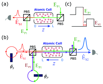
Figure 2: (Color online) Schematic diagram of experimental set up for (a) SRS: the pump field $E_{P{1}}$ generates the Stokes field $\hat{E}_{S{1}}$ and the atomic spin wave $\hat{S}_{a1}$ through spontaneous emission, and (b) CERS: after a delay $\delta t$, the leaked pump $E_{P{1}}$, acting as $E_{P{2}}$, is again injected into the vapor cell with the SRS-generated Stokes field $\hat{E}_{S{1}}$. The SRS-generated correlation of the light $\hat{E}_{S{1}}$ and the spin wave $\hat{S}_{a1}$ enhances the intensity of the second Raman Stokes field $\hat{E}_{S{2}}$. PBS: polarization beam splitter; $\phi_{P}$, $\phi_{S}$: phase shifts. (c) Time sequence for the pump pulses. $\delta t$: delay time.

Using the relations given in Eqs. (4)-(LABEL:solu3), we can compare the differences between the SRS process and CERS process by working out their output intensity in detail. In the case of the SRS, the Stokes field is generated from the vacuum and the atomic ground state without light-atom correlation. Hence the initial conditions for the SRS are  

$$\langle\hat{\mathcal{E}}_{S1}^{{\dagger}}(0,t^{\prime})\hat{\mathcal{E}}_{S1}(0,t^{\prime})\rangle =\langle\hat{S}_{a1}^{{\dagger}}(z^{\prime},0)\hat{S}_{a1}(z^{\prime},0)\rangle=0,$$ (9)

$$\langle\hat{\mathcal{E}}_{S1}(0,t^{\prime})\hat{S}_{a1}(z^{\prime},0)\rangle =0.$$ (10)

where the subscript $1$ denotes the SRS process. The detected intensity of the SRS output Stokes field at the end of the atomic cell $z^{\prime}=L$ is given by

$$I_{\text{out}}^{\text{SRS}} =\langle\hat{E}_{S1}^{(-)}\hat{E}_{S1}^{(+)}\rangle\varpropto\langle\hat{\mathcal{E}}_{S1}^{{\dagger}}(L,t^{\prime})\hat{\mathcal{E}}_{S1}(L,t^{\prime})\rangle$$

$$=L\left|\mathcal{V}_{S1}(L,t^{\prime})\right|^{2}+\left|\mathcal{F}_{S1}(L,t^{\prime})\right|^{2}$$

$$\times\langle\hat{F}_{S1}(z^{\prime\prime},t^{\prime\prime})\hat{F}_{S1}^{\dagger}(z^{\prime\prime},t^{\prime\prime})\rangle$$

$$\equiv I_{\text{spon}_{\text{1}}}.$$ (11)

The result reflects the fact that the Stokes field is generated from the spontaneous emission.

However, in the case of the CERS, one has a completely different initial condition as follows:

$$\hat{\mathcal{E}}_{S2}(0,t^{\prime})=\hat{\mathcal{E}}_{S1}(L,t^{\prime}),\text{ }\hat{S}_{a2}^{\dagger}(z^{\prime},0)=\hat{S}_{a1}^{\dagger}(L-z^{\prime},T),$$ (12)

where the subscript $2$ denotes the CERS process, $L-z^{\prime}$ indicates the opposite propagation of the two pump fields, and $T$ is the pulse duration of the pump $E_{P1}$. Evidently from Eq. (11), the light-atom correlation will play an important role in the CERS due to the relations

$$\langle\hat{\mathcal{E}}_{S2}^{{\dagger}}(0,t^{\prime})\hat{\mathcal{E}}_{S2}(0,t^{\prime})\rangle \neq 0,\text{ }\langle\hat{S}_{a2}^{{\dagger}}(z^{\prime},0)\hat{S}_{a2}(z^{\prime},0)\rangle\neq 0,\text{ }$$ (13)

$$\langle\hat{\mathcal{E}}_{S2}(0,t^{\prime})\hat{S}_{a2}(z^{\prime},0)\rangle \neq 0.$$ (14)

In general, the spin wave $\hat{S}_{a1}(z^{\prime},T)$ decays due to collisional dephasing by a factor $e^{-\Gamma_{S}\delta t}$ with $\delta t$ being the delay time. Here for convenience, we neglect the slow decay of the spin wave by assuming a short delay time ($\Gamma_{S}\delta t\ll 1$).

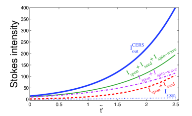
Figure 3: (Color online) The intensity of Stokes field $\hat{\mathcal{E}}_{S{2}}$ versus the dimensionless time $\tilde{t}^{\prime}$: SRS case (dotted line), seeded-light only case (dashed line), spin-wave only case (dotted-dashed line), light-atom uncorrelated case (thin solid line), and light-atom correlated case (thick solid line). The parameters are as follows: $\Delta\phi+\Delta\phi_{\text{offset}}=0$, $\mathcal{W}_{2}(0)=0.99$, $\Delta=1.2$ GHz, $|\Omega_{P{1}}|=|\Omega_{P{2}}|=2.5\times 10^{8}$ Hz, $Ng_{2}^{2}/c=1\times 10^{12}/(m\cdot s)$ , $\gamma_{s}=10$ KHz, and $\gamma_{1}=2\pi\times 5.746$ MHz.

The detected intensity of the CERS output Stokes field can be worked out

$$I_{\text{out}}^{\text{CERS}} =\langle\hat{E}_{S2}^{(-)}\hat{E}_{S2}^{(+)}\rangle\varpropto\langle\hat{\mathcal{E}}_{S2}^{{\dagger}}(L,t^{\prime})\hat{\mathcal{E}}_{S2}(L,t^{\prime})\rangle$$

$$=I_{\text{spon}}+I_{\text{seed}}+I_{\text{spin-wave}}+I_{\text{light-atom}},$$ (15)

where

$$I_{\text{spon}}=L\left|\mathcal{V}_{S2}(L,t^{\prime})\right|^{2}+\left|\mathcal{F}_{S2}(L,t^{\prime})\right|^{2}$$

$$~{}~{}~{}~{}~{}~{}\times\langle\hat{F}_{S2}(z^{\prime\prime},t^{\prime\prime})\hat{F}_{S2}^{\dagger}(z^{\prime\prime},t^{\prime\prime})\rangle,$$

$$I_{\text{seed}}=\left|\mathcal{U}_{S2}(L,t^{\prime})\right|^{2}\langle\hat{\mathcal{E}}_{S1}^{{\dagger}}(L,t^{\prime\prime})\hat{\mathcal{E}}_{S1}(L,t^{\prime\prime})\rangle,$$

$$I_{\text{spin-wave}}=\left|\mathcal{V}_{S2}(L,t^{\prime})\right|^{2}$$

$$~{}~{}~{}~{}~{}~{}\times\langle\hat{S}_{a1}^{\dagger}(L-z^{\prime\prime},T)\hat{S}_{a1}(L-z^{\prime\prime},T)\rangle,$$

$$I_{\text{light-atom}}=e^{i\Delta\phi\text{ }}\mathcal{U}_{S2}^{\ast}(L,t^{\prime})\mathcal{V}_{S2}(L,t^{\prime})$$

$$~{}~{}~{}~{}~{}~{}\times\langle\hat{\mathcal{E}}_{S1}^{{\dagger}}(L,t^{\prime\prime})\hat{S}_{a1}^{\dagger}(L-z^{\prime\prime},T)\rangle+\text{c.c.}$$ (16)

The term $I_{\text{spon}}$ originates from the same mechanism as in the SRS. The injected seeding field and the initial spin wave contribute the intensity terms $I_{\text{seed}}$ and $I_{\text{spin-wave}}$. The light-atom correlation leads to an interference term $I_{\text{light-atom}}$, which is sensitive to the phase difference $\Delta\phi\equiv\phi_{P}-\phi_{S}$, experienced by the pump and the Stokes field in CERS.

The CERS much depends on the initially-set conditions. A different setting mechanism of initial conditions results in different enhancement. For the case discussed here, this can be summarized as follows. When only seeded light (spin wave) exists, the corresponding enhancement $I_{\text{seed}}$ ($I_{\text{spin-wave}})$ occurs. Then the output intensity is

$$I_{\text{out}}=I_{\text{spon}}+I_{\text{seed (spin-wave)}},$$ (17)

The spin wave (atomic coherence) induced enhancement mechanism was studied by both theory and experiment Chen09 ; Yuan10 ; Chen10 ; Smithey . When the uncorrelated light field and the spin wave are used as the initial input seeding, the enhancement is independently contributed by the light field and the spin wave, respectively. As a result, the output intensity of the Stokes field is a simple sum given as

$$I_{\text{out}}=I_{\text{spon}}+I_{\text{seed}}+I_{\text{spin-wave}}.$$

The light-atom correlation is a new mechanism which leads to the phase-sensitive interference in the Raman scattering. It is well-known that the constructive interference can greatly enhance the light intensity. In this sense, the CERS occurs optimally for an appropriate phase difference determined by $\Delta\phi+\Delta\phi_{\text{offset}}=2n\pi$ $(n=0,1...)$, where $\Delta\phi_{\text{offset}}$ is an overall phase shift offset by the seeded light, initial spin wave and the Raman scattering process itself. In addition, we point out that the light-atom correlation also leads to a maximally reduced Raman scattering when the phase difference satisfies the condition $\Delta\phi+\Delta\phi_{\text{offset}}=(2n+1)\pi$ $(n=0,1...)$.

IV Numerical Analysis

In this section, we numerically calculate the intensities for different mechanisms of enhancement. For convenience, we define the dimensionless time $\tilde{t}^{\prime}=t^{\prime}\chi_{1}^{2}L/c=t^{\prime}\chi_{2}^{2}L/c$. According to the different scattering mechanisms, the Stokes intensities of different cases are plotted.

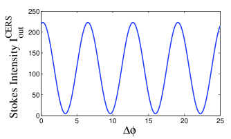
Figure 4: (Color online) The intensity of Stokes field $\hat{\mathcal{E}}_{S{2}}$ versus the relative phase $\Delta\phi$. The other parameters are the same as those of Fig. 3 except the dimensionless time at $\tilde{t}^{\prime}=2$.

In Fig. 3 the intensity determined by the SRS mechanism $I_{\text{spon}}$ is plotted as the dotted line. The contributions from the seeded light $I_{\text{seed}}$ and the spin wave $I_{\text{spin-wave}}$ are shown in the dashed and the dotted-dashed lines, respectively. The enhanced total intensity without the light-atom correlation $I_{\text{out}}=I_{\text{spon}}+I_{\text{seed}}+I_{\text{spin-wave}}$ is represented by the thin solid line. The optimal CERS output intensity $I_{\text{out}}^{\text{CERS}}$ is evidently increased due to the correlation-induced interference for the special phase difference $\Delta\phi+\Delta\phi_{\text{offset}}=0$, chosen in the calculation, where the result is displayed as a thick solid line.

Furthermore, we analyze the phase sensitivity of the CERS. In Fig. 4, we plot the intensity $I_{\text{out}}^{\text{CERS}}$ as a function of the phase difference $\Delta\phi$. This figure shows that the intensity is modulated by the relative phase $\Delta\phi$. The modulation is a reflection of the correlation-induced interference. The visibility of the interference fringes is given by $V=[(I_{\text{out}}^{\text{CERS}})_{\max}-(I_{\text{out}}^{\text{CERS}})_{\min}]/[(I_{\text{out}}^{\text{CERS}})_{\max}+(I_{\text{out}}^{\text{CERS}})_{\min}]$. In the CERS, the high visibility can be achieved by controlling the seeded light and initial spin wave to realize the case $I_{\text{seed}}=I_{\text{spin-wave}}$. A direct application of the phase-sensitive Raman scattering proposed here is to realize a nonlinear interferometer Yurke ; Jing11 , which can benefit the improvement of phase estimation for optical metrology, imaging, and information processing Cave ; Giovannetti ; Dowling .

V Conclusion

In conclusion, we have theoretically studied the correlation-induced phase-sensitive Raman scattering, which is based on the light-atom correlation through the coupling of the light field with the atomic spin excitations in the Raman scattering. We analyze the phase sensitivity of such a Raman scattering process. An optimally enhanced Raman scattering occurs when the accumulated phase difference determined by the pump, the seeded light, and the Raman process is appropriate. Similarly, one can also have a reduced Raman scattering by tuning the phase difference. Such a correlation-induced phase-sensitive Raman scattering process may find applications in a diversity of technological areas such as optical detection, metrology, imaging, precision spectroscopy, and so on.

References

• (1) R. H. Dicke, Phys. Rev. 93, 99 (1954).
• (2) D. T. Smithey, M. Belsley, K. Wedding, and M. G. Raymer, Phys. Rev. Lett. 67, 2446 (1991); M. Belsley, D. T. Smithey, K. Wedding, and M. G. Raymer, Phys. Rev. A 48, 1514 (1993).
• (3) M. Jain, H. Xia, G. Y. Yin, A. J. Merriam, and S.E.Harris, Phys. Rev. Lett. 77, 4326 (1996).
• (4) A. T. Black, James K. Thompson, and Vladan VuletiΔ‡, Phys. Rev. Lett. 95, 133601 (2005).
• (5) J. Simon, H. Tanji, J. K. Thompson, V. VuletiΔ‡, Phys. Rev. Lett. 98, 183601 (2007).
• (6) J. Simon, H. Tanji, S. Ghosh, and V. VuletiΔ‡, Nature Phys. 3, 765 (2007).
• (7) M. O. Scully, and A. A. Svidzinsky, Science 325, 1510 (2009); ibid. 328, 1239 (2010).
• (8) E. A. Sete, A. A. Svidzinsky, H. Eleuch, Z. Yang, R. D. Nevels, and M. O. Scully, J. Mod. Opt. 57, 1311 (2010).
• (9) L. Q. Chen, G. W. Zhang, Chun-Hua Yuan, J. T. Jing, Z. Y. Ou, and W. P. Zhang, Appl. Phys. Lett. 95, 041115 (2009).
• (10) L. Q. Chen, Guo-Wan Zhang, Cheng-ling Bian, Chun-Hua Yuan, Z. Y. Ou, and Weiping Zhang, Phys. Rev. Lett. 105, 133603 (2010).
• (11) G. S. Agarwal, Phys. Rev. A 83, 023802 (2011); R. Wiegner, J. von Zanthier, and G. S. Agarwal, Phys. Rev. A 84, 023805 (2011).
• (12) M. D. Lukin, P. R. Hemmer, and M. O. Scully, Adv. At., Mol., Opt. Phys. 42, 347 (2000).
• (13) R. W. Boyd, Nonlinear Optics (Academic Press, San Diego, 1992).
• (14) Chun-Hua Yuan, L. Q. Chen, J. T. Jing, Z. Y. Ou, and W. P. Zhang, Phys. Rev. A 82, 013817 (2010).
• (15) M. G. Raymer, J. Mod. Opt. 51, 1739 (2004).
• (16) W. Wasilewski, M. G. Raymer, Phys. Rev. A 73, 063816 (2006).
• (17) W. Ji, C. Wu, S. J. van Enk, and M. G. Raymer 75, 052305 (2007).
• (18) Cheng-ling Bian, L. Q. Chen, Guo-Wan Zhang, Z. Y. Ou, Weiping Zhang, Europhys. Lett. 97, 34005 (2012).
• (19) M. G. Raymer, and J. Mostowski, Physical Review A 24, 1980 (1981).
• (20) B. Yurke, S. L. McCall, and J. R. Klauder, Phys. Rev. A 33, 4033 (1985).
• (21) J. T. Jing, C. J. Liu, Z. F. Zhou, Z. Y. Ou, and W. P. Zhang, Appl. Phys. Lett. 99, 011110 (2011).
• (22) C. M. Caves, Phys. Rev. D 23, 1693 (1981).
• (23) V. Giovannetti, S. Lloyd, L. Maccone, Science 306, 1330 (2004); ibid., Nature photonics 5, 222 (2011).
• (24) J. P. Dowling, Contemporary Physics 49, 125 (2008).