Statistical mechanics of reputation systems in autonomous networks

Abstract

Reputation systems seek to infer which members of a community can be trusted based on ratings they issue about each other. We construct a Bayesian inference model and simulate approximate estimates using belief propagation (BP). The model is then mapped onto computing equilibrium properties of a spin glass in a random field and analyzed by employing the replica symmetric cavity approach. Having the fraction of trustful nodes and environment noise level as control parameters, we evaluate the theoretical performance in terms of estimation error and the robustness of the BP approximation in different scenarios. Regions of degraded performance are then explained by the convergence properties of the BP algorithm and by the emergence of a glassy phase.

Keywords: cavity and replica method; message-passing techniques; communication, supply and information networks.

1 Introduction

Ad-hoc [1] and wireless sensor networks [2] work in the absence of a central authority and are increasingly pervasive in modern computer systems. The secure operation of these autonomous networks depends on the capability of establishing trust among network entities. In general it is reasonable to assume that reputation and trust are positively correlated quantities and then employ a mutual scoring system as a source of data that can be used to estimate reputations [3, 4, 5].

Here we are concerned with the part of a reputation system [6] that identifies ill-intentioned individuals or malfunctioning devices by estimating reputations. This task would be trivial if the scores provided a reliable representation for the reputation of an entity. Instead, evaluation mistakes may happen or misleading ratings may be issued on purpose [7].

Reputation systems are particularly prone to attacks by malicious entities which can corrupt the recommendation process [8, 9, 10]. This happens for instance when multiple entities conspire to emit negative ratings about well-intentioned agents while emitting positive ratings about co-conspirators. In another form of attack, known as a Sybil attack, a single entity could impersonate others and trick the reputation mechanism.

The simplest algorithms employed by online communities use average ratings to determine reputations. Despite having the advantage of being easy to understand, these algorithms do not take into account the possibility of entities committing mistakes or acting deceitfully, what often leads to inferior results. More sophisticated algorithms employ Bayesian inference [11] or fuzzy logic [12]. Recently, iterative formulas over looped or arbitrarily long chains – the so called flow models – have also been proposed (e.g. the PageRank algorithm [13]). For a more thorough exposition of the range of techniques employed we suggest recent reviews such as [3, 10].

In this paper, we employ statistical mechanics techniques to study the performance of a belief propagation algorithm to approximately estimate reputations. This analysis provides insights into the general structure of the inference problem and suggests improvement directions.

The material is organized as follows. In section 2 we introduce the inference model, an algorithm for estimating reputations and a performance measure. In section 3 we simulate the algorithm and discuss the results. A theoretical analysis is presented in section 4 and phase diagrams are calculated. Section 5 discusses the dynamical properties of the approximate inference that impact performance. In section 6 we discuss the algorithm robustness by analyzing attacks, parameter mismatches and different topologies. Finally, conclusions are provided in section 7.

2 Estimating Reputations

We model a reputation system along the lines of [14, 15]. An entity $i=1,\cdots,n$ has a reputation $r_{i}$, and issues ratings $J_{ij}$ about other entities $j=1,\cdots,n$ with $j\neq i$. We define a set $\Omega$ of ordered pairs that contains $(i,j)$ if the rating that $i$ issues about $j$ is present. We assume that ratings and reputations are related by a given function

$$\bm{J}=f(\bm{r},\{\xi\}),$$ (1)

where $\{\xi\}$ is a set of random variables representing externalities as, for example, uncertainties affecting opinion formation or transmission. A model is defined by specifying the domains of $r_{i}$ and $J_{ij}$, the distribution of $\{\xi\}$ and the function $f$.

A good model should be able to describe realistic scenarios while remaining amenable to analytical treatment. Ratings should represent true reputations, namely, $J_{ij}\propto r_{j}$. The model should also take into account emitter reputations, as we have to consider that an unreliable entity may emit ratings defaming well-intentioned individuals or groups, and that a sufficient number of such ratings can misguide the reputation system – the collusion phenomena depicted in figure 1. A simple choice is

$$J_{ij}=\xi_{ij}r_{i}r_{j},$$ (2)

with $\xi_{ij}$ representing noise in the communication channel. We start by choosing $r_{i},J_{ij},\xi_{ij}\in\{-1,1\}$, with $\xi_{ij}$ being a random variable such that $\xi_{ij}=1$ with probability $p$ (signal level).

Figure 1: Collusion: agents of bad reputation issue positive ratings about each other and misguide the mechanism. Agents with good reputation are represented by white circles, and those of bad reputation by grey circles; arrow labels indicate whether a recommendation is positive (green) or negative (red).

This choice of $f(\bm{r},\{\xi\})$ mitigates the collusion phenomena, as $J_{ij}=-1$ represents, in the noiseless case, either an ill-intentioned positive recommendation about an unreliable entity or a negative recommendation about a reliable entity issued by an unreliable node. By introducing $\xi_{ij}$ we also build into the model misjudgments and transmission failures. We assume a prior distribution for $\bm{r}$ supposing independence and a fraction $q$ of reliable agents (reputation bias).

Our goal is to infer $\bm{r}$ given $\bm{J}$. For that we need the posterior distribution $P(\bm{r}|\bm{J})$ that can be calculated with help of Bayes theorem to find

$$P(\bm{r}|\bm{J}) \propto P(\bm{J}|\bm{r})P(\bm{r})$$

$$\propto \prod_{(i,j)\in\Omega}P(\xi_{ij})\prod_{i}P(r_{i}).$$

Notice that we can describe a $\pm 1$ random variable with probability $p$ for $x=1$ by the distribution $P(x)\propto\exp(\alpha_{p}x)$, with $\alpha_{p}=\frac{1}{2}\log\frac{p}{1-p}$. This yields

$$P(\bm{r}|J) \propto \prod_{(i,j)\in\Omega}\exp(\alpha_{p}\xi_{ij})\prod_{i}\exp(\alpha_{q}r_{i})$$ (4)

$$\propto \exp\left(\alpha_{p}\sum_{(i,j)\in\Omega}\xi_{ij}+\alpha_{q}\sum_{i}r_{i}\right)$$ (5)

$$\propto \exp\left[\alpha_{p}\left(\sum_{(i,j)\in\Omega}J_{ij}r_{i}r_{j}+\frac{\alpha_{q}}{\alpha_{p}}\sum_{i}r_{i}\right)\right],$$ (6)

where $\alpha_{q}=\frac{1}{2}\log\frac{q}{1-q}$.

Alternatively, the dependence structure of the inference model may be represented by a directed graph $\mathcal{G}=(V,E)$, with each vertex $v\in V$ standing for an entity, and an arc $(i,j)$ being connected if and only if $(i,j)\in\Omega$.

The methods of equilibrium statistical mechanics require a symmetric $\bm{J}$ which can be achieved by grouping terms as

$$\sum_{(i,j)\in\Omega}J_{ij}r_{i}r_{j}=\frac{1}{2}\sum_{ij}(J_{ij}+J_{ji})r_{i}r_{j},$$

where in the r.h.s. we assume that $J_{ij}=0$ if $(i,j)\notin\Omega$. We here only consider undirected graphs, to say, both arcs $(i,j)$ and $(j,i)$ are in $\mathcal{G}$ if $(i,j)\in\Omega$. By replacing $\frac{1}{2}(J_{ij}+J_{ji})$ for $J_{ij}$, we work with $J_{ij}\in\{-1,0,1\}$, discarding dissonant opinions that, fortunately, are few in many cases of interest [10]. The case where a single arc may be present can be modeled by a simple extension that considers $J_{ij}\in\{-1,-\frac{1}{2},0,\frac{1}{2},1\}$.

Given a sample of ratings $\{J_{ij}\}$, our goal is to find an estimate $\bm{\hat{r}}$ for the reputations $\bm{r}$ while keeping the error

$$\varepsilon(\bm{\hat{r}},\bm{r})=\frac{1}{2}\left(1-\frac{\bm{\hat{r}}\cdot\bm{r}}{n}\right),$$ (7)

as small as possible.

A naive solution calculates reputations according to the majority of recommendations (a majority rule)

$$\hat{r}_{i}=\textrm{sgn}\left(\sum_{k\in\partial i}J_{ki}\right),$$ (8)

where $\partial i$ stands for the neighborhood of the vertex $i$ in $\mathcal{G}$. Assuming that ratings are produced according to eq. 2 we can write

$$\hat{r}_{i}=\textrm{sgn}\left[\left(\sum_{k\in\partial i}\xi_{ki}r_{k}\right)r_{i}\right].$$ (9)

Thus we can calculate the probability of agreement between $\hat{r}_{i}$ and the real reputation $r_{i}$ by considering that $r_{k}$ and $\xi_{ki}$ are random variables sampled from $P(r)$ and $P(\xi)$ (while keeping $\xi_{ik}=\xi_{ki}$), and by introducing a random variable $\lambda$ sampled from the degree distribution of graph $\mathcal{G}$:

$$P(\hat{r}_{i}=r_{i}) = \Big{\langle}\!\!\Big{\langle}P\left(\sum_{k=1}^{\lambda}\xi_{ik}r_{k}>0\right)\Big{\rangle}\!\!\Big{\rangle}_{\lambda}$$ (10)

$$= \Big{\langle}\!\!\Big{\langle}\sum_{n=0}^{\lfloor\frac{\lambda-1}{2}\rfloor}{\lambda\choose n}\varpi^{(\lambda-n)}(1-\varpi)^{n}\Big{\rangle}\!\!\Big{\rangle}_{\lambda},$$

with $\varpi=pq+(1-p)(1-q)$, and $\Big{\langle}\!\!\Big{\langle}\cdot\Big{\rangle}\!\!\Big{\rangle}_{\lambda}$ denoting the average with respect to $\lambda$. Here, $\xi_{ik}r_{k}$ is a $\pm 1$ random variable with parameter $\varpi$ (i.e., it is $+1$ with probability $\varpi$). The sum of a set of these variables is binomially distributed, and the expression in the r.h.s. represents the cumulative distribution.

Until section 6 we assume a random regular graph $\mathcal{G}$ with degree $c$. Also, we deal with a scenario such that signal prevails $p>0.5$ and most of the nodes are reliable $q>0.5$.

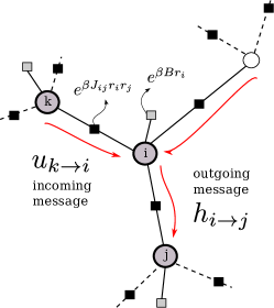
Figure 2: Factor graph and BP message-passing. Snapshot of a factor graph representing the posterior 11. Variable nodes are represented by circles, factor nodes are represented by small squares. At an iteration outgoing messages $h_{i\to j}^{(t+1)}$ are computed after combining incoming messages $u_{k\to i}^{(t)}$. When convergence is attained we compute effective fields $\hat{h}_{i}$ and the approximation for marginal posteriors $P(r_{i})$.

For an entity $i$ the inference task consists of maximizing the posterior for $\bm{r}$ marginalized over every component except $i$. The posterior is factorizable and can be put in the following form

$$P(\bm{r}|\bm{J})=\frac{1}{\mathcal{Z}}\prod_{(i,j)\in\mathcal{G}}\exp(\beta J_{ij}r_{i}r_{j})\prod_{i}\exp(\beta Br_{i}),$$ (11)

where $\beta$ and $B$ are parameters which are optimally set at Nishimori’s condition [16] $\beta=\alpha_{q}$ and $B=\frac{\alpha_{q}}{\alpha_{p}}$. Factorizable distributions such as this are well represented by factor graphs [17, 18, 19], with variable nodes associated to the $\{r_{i}\}$ and function (or factor) nodes representing the functions linking them, in this case the exponentials. Figure 2 zooms in a factor graph representation of the posterior 11.

Given this posterior distribution we calculate marginal distributions $P(r_{i})=\sum_{r_{j}\neq r_{i}}P(\bm{r}|\bm{J})$ efficiently by employing the message-passing scheme of belief propagation (BP) on the factor graph associated to the posterior eq. 11 [19]. In our case the outgoing BP messages (see figure 2 for illustration) are

$$h_{i\to j}^{(t+1)}=B+\sum_{k\in\partial i/j}u_{k\to i}^{(t)}(J_{ki},h^{(t)}_{k\to i}),$$ (12)

while $u_{k\to i}^{(t)}=\frac{1}{\beta}\tanh^{-1}\left[\tanh(\beta J_{ki})\tanh(\beta h_{k\to i}^{(t)})\right]$ are incoming messages.

Iterating this set of equations until convergence we obtain $\{h_{i\to j}^{\ast},u_{i\to j}^{\ast}\}$ that yields an approximation for marginals $P(r_{i})\propto\exp(\beta\hat{h}_{i}r_{i})$, with effective fields given by

$$\hat{h}_{i}=B+\sum_{k\in\partial i}u_{k\to i}^{\ast}.$$ (13)

This algorithm is exact on trees, but can be used in graphs of any topology, leading to good approximations provided that the average cycle length is large [19].

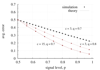
Figure 3: Estimation error for the majority rule. Average errors in simulations (circles) are compared with theoretical errors calculated by averaging eq. 7 over 10 (lines). Averages are over 3000 runs, $q=P(r_{i}=1)=0.7$ or $q=0.8$. Graphs $\cal G$ are random and regular with degree $c=3$ and $n=100$. Error bars are smaller than symbols in all three curves.

After convergence of the BP scheme reputations $r_{i}$ are estimated by marginal posterior maximization (MPM)

$$\hat{r}_{i}=\textrm{arg}\,\textrm{max}_{r_{i}}P(r_{i})=\textrm{sgn}(\hat{h}_{i}).$$ (14)

3 Simulations

As a basis of comparison we run the majority rule algorithm defined by eq. 8 for 3000 scenarios with reputations $\bm{r}$ chosen randomly with reputation bias $q$ and symmetric $\xi_{ik}$ with signal level $p$. In figure 3 we compare the average error in simulations of the majority rule with the theoretical error calculated by averaging eq. 7 over the distribution 10. The majority rule is not very far from what is used in common reputation systems on e-commerce websites. Note, however, that the error of this very simple scheme can be larger than $1-q$ if the signal level $p$ is low enough. The message is therefore clear: in noisy environments assigning good reputations by default may be actually more effective than using the majority recommendation.

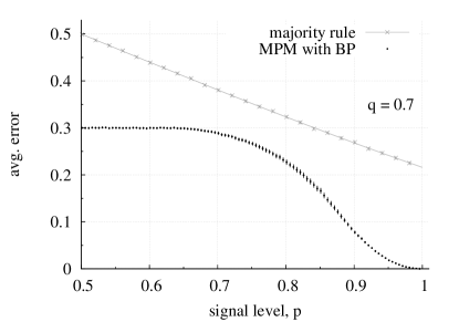
Figure 4: MPM estimate versus the majority rule. Comparison between the average error of the majority rule (eq. 8) and of the MPM estimate (eq. 14), for $q\equiv P(r_{i}=1)=0.7$, a regular random graph with degree $c=3$ and $n=100$. For the majority rule we show theory and simulations, with symbols larger than error bars. For the MPM estimate we show the average over $3000$ simulation runs with error bars representing one standard deviation.

In figure 4 we compare the majority rule with the average over $3000$ runs of the MPM estimate computed with the BP algorithm. For convenience, the algorithm is presented as a pseudocode in the A . The gains in performance when the collusion phenomena is built into the inference model are considerable even in very noisy environments.

A detailed view of the error surface for the approximate MPM estimates in terms of reputation bias $q$ and signal level $p$ is depicted in figure 5a. Two regions can be discerned with large error for low signal level (high noise) and low reputation bias. Other average quantities can also be evaluated in the simulations in order to access the algorithm’s performance. Figure 5b, for instance, shows the average number of iterations it took until convergence has been achieved. A distinctive region is observed with degraded time to convergence.

The inference algorithm has to assume (or estimate) values $\hat{p}$ and $\hat{q}$ for the signal level and reputation bias. Ideally parameters have to be set to the same values used to generate data. However, the environment can change without warning and we would also like to know how the inference scheme would perform in such circumstances. By simulation we can generate the vector $\bm{r}$ and the symmetric matrix $\xi$ as random variables with probability of being $+1$ set to $q$ and $p$, respectively, and then run the algorithm assuming $\alpha_{\hat{p}}$ and $\alpha_{\hat{q}}$.

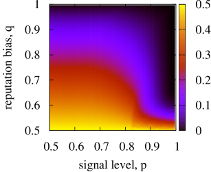
(a) average error

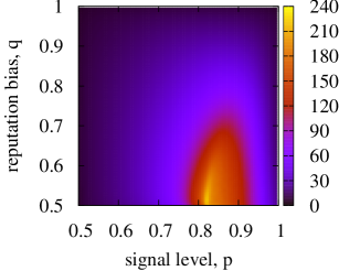
(b) iterations to convergence

Figure 5: Average error and number of iterations to convergence: $3000$ runs of the BP algorithm in a grid of values for signal level $p$ and reputation bias $q$, with $n=100$ and $c=3$. In each run $\mathcal{G}$, $\{r_{i}\}$ and $\{\xi_{ij}\}$ are sampled and ratings $\{J_{ij}=\xi_{ij}r_{i}r_{j}\}$ are calculated. Panel (a) depicts the average error as in eq. 7. Panel (b) represents the average number of iterations it took for the BP algorithm to converge.

Figure 6 depicts results of this simulations in the plane $p$–$\hat{p}$ for $q=0.6$. Small mismatches between $\hat{p}$ and $p$ are in general well absorbed by the inference scheme. A quick inspection of figure 8b reveals that for $q=0.6$, the neighborhood of $p=0.85$ exemplifies a specially sensitive region. Performance also deteriorates when estimates, in this case for the signal level, are too optimistic.

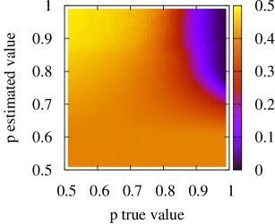
(a) empirical error

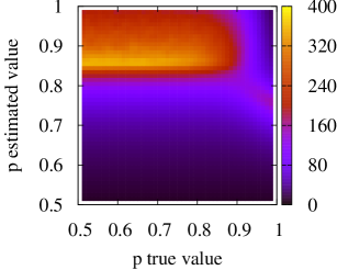
(b) iterations to convergence

Figure 6: Empirical analysis for mismatched signal level $p$ with reputation bias $q=0.6$. Panel (a): empirical error; panel (b): average number of iterations to convergence. Note that the performance is sensitive to small parameter mismatches in the neighborhood of $p=0.85$.

In the next section we use equilibrium statistical mechanics to calculate the phase diagram as a function of the control parameters $p-q$ and $p-\hat{p}$, and to explain low performance regions in both cases.

4 Theoretical analysis

The posterior distribution 6 suggests the description of the problem of inferring reputations in terms of the equilibrium properties of a spin glass in an external field

$$\mathcal{H}(\bm{s}|\bm{J},B)=-\sum_{(i,j)\in\Omega}J_{ij}s_{i}s_{j}-B\sum_{i}s_{i},$$ (15)

where we designate the dynamic variable as $s_{i}$, and the target variables $r_{i}$ are fixed (quenched). The MPM estimates described in section 3 correspond to $\hat{r}_{i}=\textrm{sgn}(m_{i})$, with $m_{i}=\tanh(\beta\hat{h}_{i})$ representing local equilibrium magnetizations.

At Nishimori’s condition [16] temperature and field are chosen as $\beta_{N}=\alpha_{p}$ and $B_{N}=\frac{\alpha_{q}}{\alpha_{p}}$, and the microstates of this physical system are distributed according to a Gibbs measure

$$P(\bm{s}|\bm{J})=\frac{1}{\mathcal{Z}}e^{-\beta_{N}\mathcal{H}(\bm{s}|\bm{J},B_{N})}$$ (16)

Other values of $\beta$ and $B$, corresponding to misspecified $p$ and $q$ can also be studied along the same lines.

We wish to calculate the equilibrium average error of eq. 7 which corresponds to the magnetization of the Hamiltonian in eq. 15 (gauge) transformed with $r_{i}s_{i}\to s_{i}$. As this Hamiltonian is not gauge invariant we now have to deal with a spin glass in a random field

$$\mathcal{H}(\bm{s}|\bm{\xi},\bm{r},B)=-\sum_{(i,j)\in\Omega}\xi_{ij}s_{i}s_{j}-B\sum_{i}r_{i}s_{i}.$$ (17)

Here $\{\xi_{ij}\}$ and $\{r_{i}\}$ are quenched variables with $P(\xi_{ij}=\xi_{ji}=1)=p$ and $P(r_{i}=1)=q$. The error $\varepsilon(\bm{\hat{r}},\bm{r})$ in the gauge transformed variables can be written as $\bar{\varepsilon}=\frac{1}{2}(1-\langle\textrm{sgn}(m)\rangle)$, where $m=\frac{1}{n}\sum_{i}s_{i}$ is the gauge transformed equilibrium magnetization.

In our analysis we employ the replica-symmetric cavity method along the lines of [19, 20]. In this section we calculate the phase diagram at Nishimori’s condition. We first write an equation for the distribution of cavity fields for the gauge transformed variables as calculated by the BP procedure in eq. 12

$$P(h)=\int\prod_{i=1}^{c-1}dh_{i}P(h_{i})\,\Big{\langle}\!\!\Big{\langle}\delta\left(h-Br-\sum_{i=1}^{c-1}u_{i}(\xi_{i},h_{i})\right)\Big{\rangle}\!\!\Big{\rangle}_{r,\{\xi_{i}\}},$$ (18)

or, more concisely

$$h\stackrel{{\scriptstyle d}}{{=}}\Big{\langle}\!\!\Big{\langle}Br+\sum_{i=1}^{c-1}u_{i}(\xi_{i},h_{i})\Big{\rangle}\!\!\Big{\rangle}_{r,\{\xi_{i}\}},$$ (19)

with $\stackrel{{\scriptstyle d}}{{=}}$ indicating equality in distribution. In this context, $h$ is the cavity field, and

$$u_{i}(\xi_{i},h_{i})=\frac{1}{\beta}\tanh^{-1}\left[\tanh(\beta\xi_{i})\tanh(\beta h_{i})\right]$$

are cavity biases [19, 21]. Note that we work here under the assumption that it makes sense to describe fixed points of the BP equations 12 in terms of a unique density $P(h)$. That is the replica symmetry (RS) assumption.

We calculate numerical solutions to 18 by the population dynamics algorithm (see B for details) and then calculate thermodynamic quantities. The magnetization is given by $m=\langle\tanh(\beta\hat{h})\rangle_{\hat{h}}$, where

$$\hat{h}\stackrel{{\scriptstyle d}}{{=}}\Big{\langle}\!\!\Big{\langle}Br+\sum_{i=1}^{c}u_{i}(\xi_{i},h_{i})\Big{\rangle}\!\!\Big{\rangle}_{r,\{\xi_{i}\}}$$ (20)

is the effective field. Note that the sum here ranges from $1$ to $c$.

The onset of a spin glass phase can be detected by finding divergences in the spin glass susceptibility. Provided that the disorder is spatially homogeneous, the spin glass susceptibility averaged over this disorder can be written as:

$$\chi_{sg}=\sum_{\ell=0}^{\infty}\mathcal{N}(\ell)\Big{\langle}\!\!\Big{\langle}\left[\langle s_{0}s_{\ell}\rangle-\langle s_{0}\rangle\langle s_{\ell}\rangle\right]^{2}\Big{\rangle}\!\!\Big{\rangle}_{r,\{\xi_{i}\},\mathcal{G}}.$$ (21)

where $s_{0}$ is a variable at an arbitrary central site, $s_{\ell}$ is an arbitrary variable at a site separated from $0$ by a chemical distance $\ell$ and $\mathcal{N}(\ell)$ is the number of sites at a distance $\ell$ from $0$.

The fluctuation-dissipation theorem, the symmetry introduced by averaging and the BP equations 12 yield

$$\chi_{sg}=\sum_{\ell=0}^{\infty}\mathcal{N}(\ell)\Big{\langle}\!\!\Big{\langle}\left[\frac{\partial m_{0}}{\partial\hat{h}_{0}}\frac{\partial\hat{h}_{0}}{\partial u_{\cdot\to 0}}\frac{\partial u_{\cdot\to 0}}{\partial u_{\cdot\to\ell}}\frac{\partial u_{\cdot\to\ell}}{\partial\hat{h}_{\ell}}\right]^{2}\Big{\rangle}\!\!\Big{\rangle}_{r,\{\xi_{i}\},\mathcal{G}},$$ (22)

where $u_{\cdot\to 0}$ and $u_{\cdot\to\ell}$ represent incoming messages in a path connecting $0$ to $\ell$. A sufficient condition for $\chi_{sg}$ to diverge is, therefore, that

$$\lim_{\ell\to\infty}\left[\frac{\partial u_{\cdot\to 0}}{\partial u_{\cdot\to\ell}}\right]^{2}>0.$$ (23)

This quantity measures the sensibility of the incoming message at a central site $0$ to a perturbation in a message forming at a far outside distance $\ell$. In terms of cavity field distributions we can write

$$\rho=\Big{\langle}\!\!\Big{\langle}\left\langle\lim_{\ell\to\infty}\left[\frac{\partial u_{0}[u_{\ell}(h)]}{\partial u_{\ell}}\right]^{2}\right\rangle_{h}\Big{\rangle}\!\!\Big{\rangle}_{r,\{\xi_{i}\}}.$$ (24)

A number of numerical methods can be used to evaluate $\rho$ [21, 20]. Using population dynamics (described in B), we introduce two slightly different initial states such that $\bm{u^{\prime}}_{0}[i]-\bm{u}_{0}[i]=\delta$ with $i=1,\cdots,N$ and $\delta=10^{-4}$. After a large number $\tau$ of iterations of the population dynamics algorithm we calculate

$$\rho\approx\frac{1}{N}\sum_{i}(\bm{u^{\prime}}_{\tau}[i]-\bm{u}_{\tau}[i])^{2}.$$ (25)

The order parameters $m$ and $\rho$ allow the identification of four different thermodynamic phases: paramagnetic if $\rho=0$, $m=0$, ferromagnetic if $\rho=0$, $m>0$, glassy if $\rho\neq 0$, $m=0$ and, mixed or ferromagnetic ordered spin glass for $\rho\neq 0$, $m>0$.

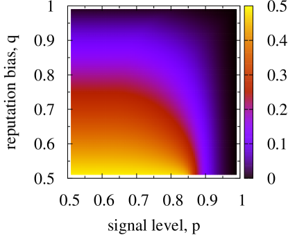
Figure 7: Theoretical error at Nishimori’s condition: theoretical error $\bar{\varepsilon}=\frac{1}{2}\left(1-\langle\textrm{sgn}(\hat{h})\rangle_{\hat{h}}\right)$ for different values of $p$ and $q$.

To measure the theoretical error, we also calculate $\langle\textrm{sgn}(\hat{h})\rangle_{\hat{h}}$. The theoretical results depicted in figure 7 are corroborated by simulations depicted in figure 5a . Under Nishimori’s condition, $\rho=0$ for all values of $p$ and $q$, and thus no glassy or mixed phase is present. Likewise, for all values of $p,q>0.5$, $m>0$, and the ferromagnetic phase covers the whole region.

Three rigorous results on phase diagrams of similar models are available: (A) if the Hamiltonian is gauge invariant the Nishimori line does not cross a spin glass phase [22]; (B) there is no spin glass phase in a random field Ising model [23]; and (C) provided that the parameters employed in the inference task are identical to those used to generate data (namely, we are at Nishimori’s condition), in a random graph with bounded maximum degree the BP scheme converges to the correct marginals in the thermodynamic limit [24].

In order to check our results we observe that choosing $q=1/2$ ($\alpha_{q}=0$) yields a gauge invariant model. Consistently with result (A), $\rho\approx 0$ over the line $q=0.5$ and only paramagnetic and ferromagnetic phases are observed with a transition around $p_{c}\approx 0.853$ for our example (see figure 7). Result (B) is only relevant if we can choose parameters such that $\xi_{ij}\geq 0$ (or $p=1$) for any $(i,j)\in\Omega$, any random field $r_{ij}$ and any $B$ in the Hamiltonian 17. At Nishimori’s condition, however, $p=1$ implies that $\beta_{N}=\infty$ and $B_{N}=0$. Thus the model is a trivial ferromagnet and result (B) is irrelevant. Yet if the inference model assumes $\hat{p}<1$ while $\xi_{ij}$ are generated with $p=1$, rigorous result (B) forbids either a spin glass or a mixed phase to show up. Accordingly, figure 8b exemplifies a phase diagram for $q>0.5$ with no mixed phase for $p=1$ (true value) and $\hat{p}<1$ (estimated value). Finally result (C) implies in the absence of a mixed phase anywhere at the Nishimori condition, which is indeed found as $\rho\approx 0$ .

This theoretical analysis may be repeated for the mismatched parameters case introduced in the previous section, by setting $\beta=\alpha_{\hat{p}}$ and $B=\frac{\alpha_{\hat{q}}}{\alpha_{\hat{p}}}$ while considering $r_{i}$ and $\xi_{i}$ as quenched $\pm 1$ random variables with parameters $q$ and $p$. Here again, the theoretical error obtained reproduces the empirical one. In the $p-\hat{p}$ plane, however, a mixed phase appears for a region of parameters. In this region, the free energy landscape becomes rugged, and BP will hardly converge to its global minimum. Also the RS cavity analysis does not necessarily provide asymptotically correct results, so the thermodynamic quantities computed in this region may not reflect the actual behavior of the system at equilibrium.

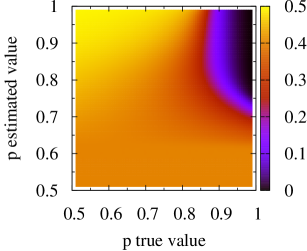
(a) theoretical error

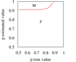
(b) phase diagram

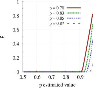
(c) $\rho$ as a function of $\hat{p}$

Figure 8: Theoretical analysis for mismatched signal level $p$ with reputation bias $q=0.6$. Panel (a): theoretical error, in good agreement with simulations. Panel (b): phase diagram, in which a mixed phase appears, explaining the algorithm’s degraded performance in that region. Panel (c): $\rho$ signals the onset of the mixed phase as $\hat{p}$ increases.

The onset of a mixed phase explains in part the degradation in algorithm’s performance for the upper left corner of the $p-\hat{p}$ plane. However, empirical results show that convergence rates also worsens outside this region of parameters, as well as on the $p-q$ plane even at Nishimori’s condition, where no glassy phase is to be found. In the next section, we investigate this issue further.

5 Dynamical properties

In order to understand such deterioration in the algorithm’s performance, we have studied the BP dynamical system. From 12, we obtain

$$\frac{\partial h_{i\to j}^{(t+1)}}{\partial h_{k\to i}^{(t)}}=\frac{\tanh(\beta)J_{ki}}{\cosh^{2}(\beta h_{k\to i}^{(t)})-\tanh^{2}(\beta)\sinh^{2}(\beta h_{k\ \to i}^{(t)})}\mathbb{I}(k\in\partial i/j).$$ (26)

The dynamical system in question has $nc$ equations, one for each direction of each edge on the graph. In order to study the linear stability of the BP dynamical system, we have calculated the spectral radius of the Jacobian matrix evaluated at a fixed point, that is, $R=\max|\lambda(\mathbb{J})|$, where $\mathbb{J}$ is a $nc\times nc$ matrix with entries $\mathbb{J}_{ij,ki}=\frac{\partial h_{i\to j}^{\ast}}{\partial h_{k\to i}^{\ast}}$.

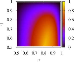
(a) Nishimori condition

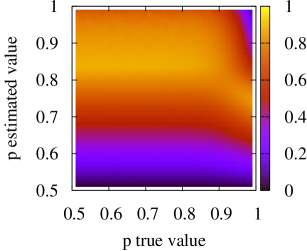
(b) mismatched $p$

Figure 9: Average spectral radius of the Jacobian of the BP dynamical system. For each value of $p$ and $q$ ($p$ and $\hat{p}$), the Jacobian’s spectral radius was computed for 2500 runs of the algorithm and then averaged. Larger values of $R$ correlate with slower convergence times. Panel (a): at Nishimori’s condition, to be compared with 5b. Panel (b): with a mismatch between $p$ and $\hat{p}$, to be compared with 6b.

The spectral radius gives us a measure of the convergence rate of the algorithm. In fact, as figure 9 shows, regions where the value of $R$ is larger coincide with those where the algorithm converges more slowly, in average.

Interestingly, this quantity may be also studied within the RS cavity scheme. The population dynamics algorithm, which we have used to obtain samples of $P(h)$, may be also seen as a dynamical system (the so called, density evolution equations):

$$\left\{\begin{array}[]{l l}u_{i}^{(\ell)}&=\frac{1}{\beta}\tanh^{-1}\left[\tanh(\beta\xi)\tanh(\beta h_{i}^{(\ell)})\right],\\ h_{i}^{(\ell+1)}&=Br+\sum_{j=1}^{c-1}u_{\gamma(j)}^{(\ell)},\\ \end{array}\right.$$ (27)

with $r$ and $\xi$ independently sampled for each $i$, and $\gamma(\cdot)$ representing random indices, that is $\gamma(\cdot)\sim\textrm{Uniform}([N])$.

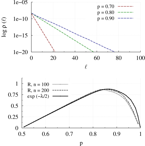
Figure 10: Decay of $\rho(\ell)$. Top panel: using population dynamics we find the rate $\lambda$ of decay as a function of $p$ for $q=0.6$. Bottom panel: the average spectral radius $R$ for finite size ($n=100,200$) maps are closely related to $e^{-\lambda/2}$. Notice the finite size effect in the large $p$ region.

In this context, the evolution of the order parameter $\rho$, $\rho(\ell)=\frac{1}{N}\sum_{i=1}^{N}({u_{i}^{\prime}}^{(\ell)}-{u_{i}}^{(\ell)})^{2}$, can be studied. As it can be seen in figure 10, $\rho(\ell)$ decays exponentially at a constant rate $\lambda$, that is, $\rho\propto e^{-\lambda\ell}$. In the neighborhood of a fixed point the decay rate of $\sqrt{\rho}$ is given by the dominant eigenvalue of the Jacobian matrix. We thus expect the relation $R\propto e^{-\frac{\lambda}{2}}$ to hold, where $R$ is the spectral radius of the Jacobian matrix. This relationship is clearly discerned in figure 10 — thus by computing the decay rate $\lambda$ for $\rho$, we also learn about the algorithm convergence rate.

We have observed two mechanisms leading to performance degradation: the onset of a glassy phase and the decreased stability of the BP fixed point. The former is a limitation intrinsic to the inference problem, the latter an issue that probably could be addressed by modifying the approximate inference algorithm. We however observe that the stability of the fixed point decreases as the parameters approach a mixed phase, as $p=0.8536,q=0.5$ defines a multicritical point in a model with $c=3$ [20], thus suggesting this can also be an intrinsic limitation of the problem.

6 Robustness

To this point our analysis has only considered ratings $\{J_{ij}\}$ distributed over a regular random graph of fixed degree $c=3$ and issued exactly as assumed by the inference model. In this section, we relax these assumptions to access both the performance of the algorithm and the validity of the theoretical analysis under more general conditions.

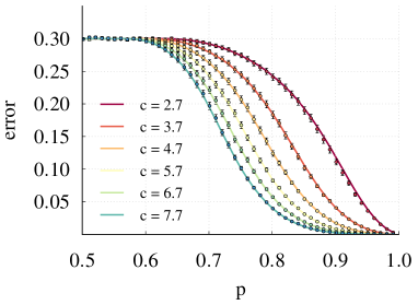
(a) empirical error

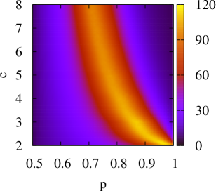
(b) iterations to convergence

Figure 11: Empirical and theoretical analysis at Nishimori’s condition for a random graph with degree distribution given by eq. 28 and $q=0.7$. The parameter $c$ is the average node degree while $p$ is the signal level. Panel (a) compares empirical (bars) and theoretical (lines) errors as a function of $p$ for (from top to bottom) $c=2.7$ to $c=7.7$ in steps of size $1$ . Panel (b) depicts the average number of iterations for the BP algorithm to converge.

6.1 Graph topologies

The set $\Omega$ of ratings issued by network entities define a graph $\mathcal{G}$ with each vertex representing an entity and an edge $(i,j)$ being connected if and only if $(i,j)\in\Omega$. The theoretical analysis based on the replica-symmetric cavity equation 18 relies on specifying an ensemble of graphs represented by a particular degree distribution (or profile). In the previous discussion we have used an ensemble of regular random graphs with a degree profile given by $\Lambda_{c}(\gamma)=\delta\,(\gamma-c)$. A natural extension to that is allowing non-integer values of $c$, for that we introduce:

$$\Lambda_{c}(\gamma)=\left\{\begin{array}[]{l l}1-(c-\lfloor c\rfloor)&\quad\textrm{for $\gamma=\lfloor c\rfloor$,}\\ c-\lfloor c\rfloor&\quad\textrm{for $\gamma=\lfloor c\rfloor+1$,}\\ 0&\quad\textrm{otherwise.}\end{array}\right.$$ (28)

In this way for $c=2.3$ we would have 30% of the nodes with degree 3 and the remaining with degree 2.

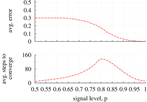
Figure 12: Simulations in a square lattice, for $q=0.7$ and different values of $p$. Despite the short cycle lengths, the algorithm exhibits a good performance.

The empirical analysis is done by simulating instances sampled from this ensemble of graphs. Figure 11(a) compares empirical and theoretical errors at Nishimori’s condition as a function of $p$ for several $c$ values, $q=0.7$. Figure 11(b) depicts the average number of iterations to convergence as a function of $p$ and $c$ which is explained by the stability of the unique BP fixed point.

The BP algorithm calculates exact marginals and allows for optimal Bayesian inference when the subjacent graph is a tree. The performance of the BP algorithm, however, can be studied by simulation on any topology. Figure 12 shows the resulting performance measures as a function of $p$ for $q=0.7$ and for $\mathcal{G}$ chosen to be a square lattice in two dimensions. The average error is always smaller than $1-q$ and vanishes as $p\rightarrow 1$ showing that even in this case the BP algorithm may yield good results.

6.2 Attacks

Malicious entities may issue ill-intentioned ratings to trick the reputation system and malfunctioning devices may issue erroneous ratings. These scenarios of targeted attacks can also be considered by the inference model and studied within the same theoretical framework and simulation techniques.

We suppose that a fraction $f$ of the ratings are issued by noisy entities while the inference process remains unchanged. Lets call the subset of noisy ratings $\Omega_{f}\subset\Omega$. To simulate this scenario, we uniformly sample and fix a fraction $\frac{f}{2}$ of the entities to be noisy, issuing ratings as $J_{ij}=\eta_{ij}$, where $\eta_{ij}=\eta_{ji}$ is a $\pm 1$ random variable with parameter $z=\frac{1}{2}$ and $(i,j)\in\Omega_{f}$ — since we require $J_{ji}=J_{ij}$, the total fractions of noisy ratings will be $f$. We then run the BP algorithm and study how the performance changes with $f$.

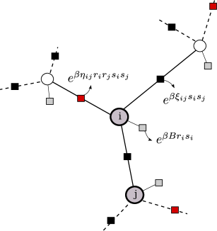
Figure 13: Factor graph for the posterior 30. A fraction $f$ of the function nodes represent noisy ratings (red squares).

For the theoretical analysis we calculate performance measures averaged over every disorder component: regular random graph with $c=3$ in our example, symmetric communication noise $\bm{\xi}$, symmetric random ratings $\bm{\eta}$ and symmetric ratings $\bm{J}$. As we are interested in checking algorithm robustness, we also assume that the inference scheme has no knowledge that the reputation system is under attack.

We first rewrite the posterior by taking into account noisy ratings:

$$P(\bm{r}|J)\propto\prod_{(i,j)\in\Omega\setminus\Omega_{f}}P(\xi_{ij})\prod_{(i,j)\in\Omega_{f}}P(\eta_{ij})\prod_{i}P(r_{i}).$$ (29)

Following the previous steps yields:

$$P(\bm{r}|J)\propto e^{\alpha_{p}\sum_{(i,j)\in\Omega\setminus\Omega_{f}}J_{ij}r_{i}r_{j}}e^{\alpha_{z}\sum_{(i,j)\in\Omega_{f}}\eta_{ij}+\alpha_{q}\sum_{i}r_{i}}$$ (30)

Since the algorithm considers the ratings $\Omega_{f}$ as subject to the same communication noise as regular ratings, we have $\alpha_{z}=\alpha_{p}$. The gauge transformed Hamiltonian for an equilibrium statistical mechanics description is

$$H(\bm{s})=-\sum_{(i,j)\in\Omega\setminus\Omega_{f}}\xi_{ij}s_{i}s_{j}-\sum_{(i,j)\in\Omega_{f}}\eta_{ij}r_{i}r_{j}s_{i}s_{j}-B\sum_{i}r_{i}s_{i}.$$ (31)

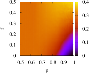
(a) empirical error

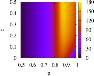
(b) iterations to convergence

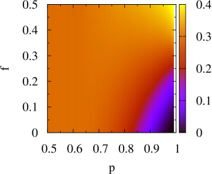
(c) theoretical error

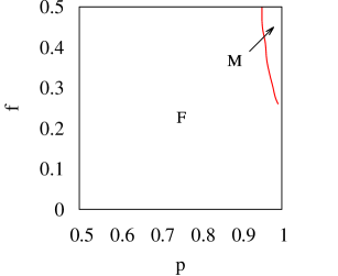
(d) phase diagram

Figure 14: Fraction $f$ of nodes broadcasting random ratings. Panels (a) and (b) depict simulation results for the error and for the average number of iterations to convergence. Panels (c) and (d) show theoretical error and phase diagram using the replica symmetric cavity approach. As expected, the error increases with $f$.

There is a new term $-\sum_{(i,j)\in\Omega_{f}}\eta_{ij}r_{i}r_{j}s_{i}s_{j}$ in the Hamiltonian, which can be treated by the inclusion of a new type of function node to the factor graph representation for the posterior 30. Figure 13 provides a snapshot of this factor graph. The replica symmetric cavity description can then be written as

$$h\stackrel{{\scriptstyle d}}{{=}}\Big{\langle}\!\!\Big{\langle}Br+\sum_{i=1}^{c-1}u_{i}(h)\Big{\rangle}\!\!\Big{\rangle}_{r,\xi,\eta},$$ (32)

where $u_{i}(h)=\frac{1}{\beta}\tanh^{-1}\left[\tanh(\beta\xi_{i})\tanh(\beta h_{i})\right]$ with probability $1-f$, and with probability $f$

$$u_{i}(h)=\frac{1}{\beta}\tanh^{-1}\left[\tanh(\beta\eta_{i}rr_{i})\tanh(\beta h_{i})\right],$$

where $\eta_{i}$ is a $\pm 1$ random variable with $P(\eta_{i}=1)=\frac{1}{2}$, $r$ is the same used in eq. 32 and the $\{r_{i}\}$ are independently sampled from $r$.

Figure 14 depicts simulation results for the error in Panel (a) and for the number of iterations to convergence in Panel (b). Panels (c) and (d) show theoretical error and phase diagram using the replica symmetric cavity approach. The increased time to convergence inside the ferromagnetic phase is explained by the decreased stability of the still unique BP fixed point. Inside the mixed phase new fixed points emerge and the inference process is fundamentally faulty as can be seen in the top right corner of the error surface.

7 Conclusions

The use of a belief propagation (BP) algorithm for approximate inference in reputation systems has been introduced in [25, 26]. We here extend previous work by calculating performance measures using the replica symmetric cavity approach after expressing the inference problem in terms of equilibrium statistical mechanics. We apply this framework to a basic scenario and to three simple variations.

The framework is very general and allows for the study of the algorithm performance when subjected to several scenarios of practical interest such as the presence of collusions, parameter mismatches and targeted attacks. Other questions of practical interest remain. Algorithms based on BP approximate inference seem to represent an interesting alternative for reputation systems such as wireless sensor networks, however implementation details that have been purposefully ignored in our analysis certainly deserve a more thorough analysis. For instance, sensors often operate with very limited resources, so that sampling of ratings and running of the algorithm should be scheduled taking these limitations into account. Also faulty elements would behave differently with lower signal to noise rates. In another direction, in a distributed scheme it would be interesting to study the role of different prescriptions for the matrix $\bm{J}$.

From a theoretical point of view reinforced belief propagation or survey propagation techniques promise better results in the deteriorated performance glassy phase. Also, expectation maximization-belief propagation [27] could allow the algorithm to run without the need of supplying signal level $p$ and reputation bias $q$ as inputs. For scenarios involving targeted attacks more information could be built into the rating mechanism that may allow for improved inference algorithms.

Appendix A Computation of marginals using belief propagation

The algorithm takes as input a distribution $P(h)$ from which the messages are initially sampled, a maximum to the number of iterations $t_{\max}$, a precision $\epsilon$ for convergence and estimated values of $p$ and $q$, $\{\hat{p},\hat{q}\}$. In what follows, we have used $P^{(0)}(h)=\delta(h)$, $t_{\max}\sim 100$, $\epsilon\sim 10^{-7}$ and $\{\hat{p},\hat{q}\}=\{p,q\}$ — this last condition is later relaxed. The complete pseudocode is as follows:

0:  $P^{(0)}(h)$, $t_{\max}$, $\epsilon$, $\{\hat{p},\hat{q}\}$; $\{J_{ij}\}$, $\mathcal{G}$

0:  $\{\hat{r}_{i}\}$

1:  initialize $\{h_{i\to j}\}$ sampling from $P^{(0)}(h)$

2:  $\beta\leftarrow\alpha_{\hat{p}}$, $B\leftarrow{\alpha_{\hat{q}}}/{\alpha_{\hat{p}}}$

3:  while $\Delta\geq\epsilon$ and $t<t_{\max}$ do

4:     for $i=1\to n$, $j\in\partial i$ do

5:        $h_{i\to j}^{\prime}=B+\sum_{k\in\partial i/j}u_{k\to i}(J_{ki},h_{k\to i})$

6:     end for

7:     $\Delta\leftarrow\max\,|h_{i\to j}^{\prime}-h_{i\to j}|$

8:     $t\leftarrow t+1$, $\{h_{i\to j}\}\leftarrow\{h_{i\to j}^{\prime}\}$

9:  end while

10:  if $\Delta<\epsilon$ then

11:     for $i=1$ to $n$ do

12:        $\hat{h}_{i}=B+\sum_{k\in\partial i}u_{k\to i}(J_{ki},h_{k\to i})$

13:        $\hat{r}_{i}=\textrm{sgn}(\hat{h}_{i})$

14:     end for

15:  end if

Appendix B Population dynamics

The population dynamics algorithm provides an approximate solution to 19 by iterating

$$\left\{\begin{array}[]{l l}u_{i}^{(\ell)}&=\frac{1}{\beta}\tanh^{-1}\left[\tanh(\beta\xi)\tanh(\beta h_{i}^{(\ell)})\right],\\ h_{i}^{(\ell+1)}&=Br+\sum_{j=1}^{c-1}u_{j}^{(\ell)}.\\ \end{array}\right.$$ (33)

We introduce two arrays of length $N=10^{4}$: $\bm{h}$ and $\bm{u}$. At the first step, the elements of $\bm{u}$ are initialized. We have considered two possible ways of initializing $\bm{u}$: by uniformly sampling from $[-\varepsilon,\varepsilon]$, $\varepsilon=10^{-2}$, or by assigning $u_{i}^{(0)}=\xi_{i}$ (i.e., $\tanh(\beta h_{i}^{(0)})=1$); the results obtained in our analysis were very similar for both. For discussions regarding the use of different initial conditions, the reader may refer to [21, 20].

Next, the elements of $\bm{h}$ are updated according to the rule, with $\{u_{j}\}$ uniformly sampled from $\bm{u}$ and $r$ sampled from $P(r)$; and the elements of $\bm{u}$ are calculated from the respective element in $\bm{h}$ and $\xi$ sampled from $P(\xi)$. The process is repeated $\tau=5000$ times. After this large number of iterations, the array $\bm{h}$ should be approximately distributed as the real distribution $P(h)$, and we are then able to calculate the desired averages.

In order to calculate $m=\left\langle\tanh(\beta\hat{h})\right\rangle_{\hat{h}}$, we may introduce an array $\bm{\hat{h}}$ with the same length $N$, and since $\hat{h}$ is given by a sum with an extra term, the array elements are computed by simply summing the elements of $\bm{h}$ with some uniformly sampled element of $\bm{u}$. We then have $m\approx\frac{1}{N}\sum_{i}\tanh(\bm{\hat{h}}[i])$.

References

References

- [1] M. Barbeau and E. Kranakis. Principles of Ad Hoc Networking. Wiley, 2007.
- [2] W. Dargie and C. Poellabauer. Fundamentals of Wireless Sensor Networks: Theory and Practice. Wiley, 2010.
- [3] J. Sabater and C. Sierra. Review on Computational Trust and Reputation Models. Artificial Intelligence Review, 24(1):33–60, September 2005.
- [4] L. Mui. Computational Models of Trust and Reputation: Agents, Evolutionary Games, and Social Networks. PhD thesis, Massachusetts Institute of Technology, 2002.
- [5] E. Buchmann. Trust Mechanisms and Reputation Systems. In Dorothea Wagner and Roger Wattenhofer, editors, Algorithms for Sensor and Ad Hoc Networks, pages 325–336. Springer, Berlin, 2007.
- [6] F. G. Marmol and G. M. Pérez. Towards pre-standardization of trust and reputation models for distributed and heterogeneous systems. Computer Standards & Interfaces, 32(4):185–196, June 2010.
- [7] A. Josang and J. Golbeck. Challenges for robust of trust and reputation systems. In Proceedings of the 5th International Workshop on Security and Trust Management, number September, 2009.
- [8] F. G. Marmol and G. M. Pérez. Security threats scenarios in trust and reputation models for distributed systems. Computers & Security, 28(7):545–556, October 2009.
- [9] K. Hoffman, D. Zage, and C. Nita-Rotaru. A survey of attack and defense techniques for reputation systems. ACM Computing Surveys, 42(1), December 2009.
- [10] A. Jøsang, R. Ismail, and C. Boyd. A survey of trust and reputation systems for online service provision. Decision Support Systems, 43(2):618–644, March 2007.
- [11] L. Mui, A. Halberstadt, and M. Mohtashemi. Notions of Reputation in Multi-Agents Systems: A Review. In Proceedings of AAMAS ’02, pages 280–287, New York, USA, 2002. ACM Press.
- [12] J. Sabater and C. Sierra. REGRET: reputation in gregarious societies. In Proceedings of AGENTS ’01, pages 194–195, New York, USA, 2001. ACM Press.
- [13] L. Page, S. Brin, R. Motwani, and T. Winograd. The PageRank Citation Ranking: Bringing Order To The Web. Technical report, Stanford University, 1998.
- [14] S. Ermon, L. Schenato, and S. Zampieri. Trust Estimation in autonomic networks: a statistical mechanics approach. In Proceedings of the 48th IEEE Conference on Decision and Control (CDC), pages 4790–4795, December 2009.
- [15] T. Jiang and J. S. Baras. Trust evaluation in anarchy: A case study on autonomous networks. In Proceedings of IEEE Infocom, 2006.
- [16] Y. Iba. The Nishimori line and Bayesian statistics. J. Phys. A: Math. Gen., (32):3875–3888, 1999.
- [17] F.R. Kschischang, B.J. Frey, and H.-A. Loeliger. Factor graphs and the sum-product algorithm. Information Theory, IEEE Transactions on, 47(2):498 –519, feb 2001.
- [18] H.-A. Loeliger. IEEE Signal Processing Magazine, January 2004.
- [19] M. Mezard and A. Montanari. Information, Physics, and Computation. Oxford University Press, USA, 2009.
- [20] Y. Matsuda, H. Nishimori, L. Zdeborová, and F. Krzakala. Random-field p-spin-glass model on regular random graphs. Journal of Physics A: Mathematical and Theoretical, 44(18):185002, May 2011.
- [21] L. Zdeborová. Statistical physics of hard optimization problems. Acta Physica Slovaca. Reviews and Tutorials, 59(3):169–303, June 2009.
- [22] H. Nishimori. Statistical Physics of Spin Glasses and Information Processing. Oxford University Press, 2001.
- [23] F. Krzakala, F. Ricci-Tersenghi, and L. Zdeborová. Elusive spin-glass phase in the random field ising model. Physical Review Letters, 104:207208, 2010.
- [24] A. Montanari. Estimating random variables from random sparse observations. European Transactions on Telecommunications, 19(4):385–403, 2008.
- [25] S. Ermon. Trust Estimation in autonomic networks: a message passing approach. In Proceedings of NECSYS, Venice, 2009, 2009.
- [26] E. Ayday. Application of belief propagation to trust and reputation management. In Proceedings of IEEE International Symposium on Information Theory (ISIT), pages 2173–2177, July 2011.
- [27] A. Decelle, F. Krzakala, C. Moore, and L. Zdeborová. Asymptotic analysis of the stochastic block model for modular networks and its algorithmic applications. Physical Review E, 84(6):1–25, December 2011.