Near Threshold Neutral Pion Electroproduction at High Momentum Transfers and Generalized Form Factors

Abstract

We report the measurement of near threshold neutral pion electroproduction cross sections and the extraction of the associated structure functions on the proton in the kinematic range $Q^{2}$ from $2$ to $4.5$ GeV² and $W$ from $1.08$ to $1.16$ GeV. These measurements allow us to access the dominant pion-nucleon $s$-wave multipoles $E_{0+}$ and $S_{0+}$ in the near-threshold region. In the light-cone sum-rule framework (LCSR), these multipoles are related to the generalized form factors $G_{1}^{\pi^{0}p}(Q^{2})$ and $G_{2}^{\pi^{0}p}(Q^{2})$. The data are compared to these generalized form factors and the results for $G_{1}^{\pi^{0}p}(Q^{2})$ are found to be in good agreement with the LCSR predictions, but the level of agreement with $G_{2}^{\pi^{0}p}(Q^{2})$ is poor.

I Introduction

Pion photo- and electroproduction on the nucleon $\gamma N\to\pi N$, $\gamma^{*}N\to\pi N$ close to threshold has been studied extensively since the 1950s both experimentally and theoretically. Exact predictions for the threshold cross sections and the axial form factor were pioneered by Kroll and Ruderman in 1954 for photo-production and are known as the low energy theorem (LET) Kroll and Ruderman (1954). This LET provided model independent predictions of cross sections for pion photoproduction in the threshold region by applying gauge and Lorentz invariance Drechsel and Tiator (1992). This was the first of the LET predictions to appear but was not without limitations. This LET predictions were restricted only to charged pions and the $\pi^{0}$ contribution was shown to vanish in the ‘soft pion’ limit, i.e., $m_{\pi}\sim p_{\pi}$. Here, $m_{\pi}$ and $p_{\pi}$ are the mass and momentum of the pion. Additionally, these cross section predictions were limited to diagrams with first order contributions in the pion-nucleon mass ratio. In later years, using vanishing pion mass chiral symmetry ($m_{\pi}\to 0$), these predictions were extended to pion electroproduction for both charged and neutral pions Nambu and Lurié (1962); Nambu and Shrauner (1962).

Of course, a vanishing pion mass doesn’t relate to the observed mass of the pion (the pion to nucleon mass ratio $m_{\pi}/m_{N}\sim 1/7$), so higher order finite mass corrections to the LET were formulated in the late sixties and early seventies before the appearance of QCD. These also included contributions to the non-vanishing neutral pion amplitudes for the cross section.

In the late eighties and early nineties, experiments at Mainz Beck et al. (1990) obtained threshold pion photo-production data on $\gamma p\to\pi^{0}p$. The theoretical predictions of LETs at the time were inconsistent with the data at low photon energies. With the emergence of chiral perturbation theory ($\chi$PT), the scattering amplitudes and some physical observables were systematically expanded in the low energy limit in powers of pion mass and momentum. Using this framework, the LET was re-derived to include contributions to the amplitudes from certain loop diagrams, which were lost when the expansion was performed in terms of the pion mass, as was done in the earlier works Vainshtein and Zakharov (1972); Scherer and Koch (1991). Further electroproduction experiments at NIKHEF Welch et al. (1992) on $\gamma^{*}p\to\pi^{0}p$ with photon virtuality $Q^{2}\sim 0.05-0.1$ GeV² provided good agreement with $\chi$PT predictions.

These LETs Kroll and Ruderman (1954); Nambu and Lurié (1962); Nambu and Shrauner (1962); Vainshtein and Zakharov (1972); Scherer and Koch (1991) are not applicable for $Q^{2}\gg\Lambda_{QCD}^{3}/m_{\pi}$, where $\Lambda_{QCD}\sim 200-300$ MeV is the QCD scale parameter. In the case of asymptotically large momentum transfers ($Q^{2}\to\infty$) perturbative QCD (pQCD) factorization techniques Pobylitsa et al. (2001); Efremov and Radyushkin (1980); Lepage and Brodsky (1980) have been used to obtain predictions for cross section amplitudes and axial form factors near threshold. In these factorization techniques, ‘hard’ ($Q^{2}\gg\Lambda^{2}_{QCD}$) and ‘soft’ ($k\sim\Lambda_{QCD}$) momentum contributions to the scattering amplitude can be separated cleanly and each contribution can be theoretically calculated using pQCD and LETs, respectively. Here, $k$ is the momentum of the virtual photon.

Recently, Braun et al. Braun et al. (2007, 2008) suggested a method to extract the generalized form factors, $G_{1}^{\pi N}(Q^{2})$ and $G_{2}^{\pi N}(Q^{2})$, for $1<Q^{2}<10$ GeV² using light cone sum rules (LCSR). The transition matrix elements of the electromagnetic interaction, $J_{\mu}$, can be written in terms of these form factors at threshold:

$$\langle N(P^{\prime})\pi(k)|J_{\mu}|p(P)\rangle=-\frac{i}{f_{\pi}}\bar{N}\gamma_{5}\left[(\gamma_{\mu}q^{2}-q_{\mu}\not{q})\frac{G_{1}^{\pi N}(Q^{2})}{m_{N}^{2}}-\frac{i\sigma_{\mu\nu}q^{\nu}}{2m_{N}}G_{2}^{\pi N}(Q^{2})\right]p.$$ (1)

Here, $N(P^{\prime})$ and $p(P)$ are spinors for the final and initial nucleons with momenta $P^{\prime}$ and $P$, respectively, $m_{N}$ is the mass of the nucleon, $f_{\pi}$ is the pion decay constant and $q$ is the 4-momentum of the virtual photon. Since the pion is a negative parity particle and the electromagnetic current is parity conserving, the $\gamma_{5}$ matrix is present to conserve the overall parity of the reaction.

These form factors are directly related to the pion-nucleon $s$-wave multipoles $E_{0+}$ and $L_{0+}$ Braun et al. (2007, 2008)

$$E_{0+} = \frac{\sqrt{4\pi\alpha}}{8\pi f_{\pi}}\sqrt{\frac{(2m_{N}+m_{\pi})^{2}+Q^{2}}{m_{N}^{3}(m_{N}+m_{\pi})^{3}}}$$ (2)

$$\times\left(Q^{2}G_{1}^{\pi N}-\frac{m_{N}m_{\pi}}{2}G_{2}^{\pi N}\right)$$

$$L_{0+} = \frac{\sqrt{4\pi\alpha}}{8\pi f_{\pi}}\frac{m_{N}|\omega^{th}_{\gamma}|}{2}\sqrt{\frac{(2m_{N}+m_{\pi})^{2}+Q^{2}}{m_{N}^{3}(m_{N}+m_{\pi})^{3}}}$$ (3)

$$\times\left(G_{2}^{\pi N}+\frac{2m_{\pi}}{m_{N}}G_{1}^{\pi N}\right).$$

Here, $\alpha$ is the electromagnetic coupling constant and $\omega_{\gamma}^{th}$ is the virtual photon energy at threshold in the c.m. frame and is given by the following relation:

$$\omega^{th}_{\gamma}=\frac{m_{\pi}(2m_{N}+m_{\pi})-Q^{2}}{2(m_{N}+m_{\pi})}.$$ (4)

In general, $E_{l\pm}$, $M_{l\pm}$, and $L_{l\pm}$ describe the electric, magnetic and longitudinal multipoles, respectively. Here, $l$ describes the total orbital angular momentum of the pion relative to the nucleon and $\pm$ is short for $\pm\frac{1}{2}$ so that the total angular momentum of the $\pi N$ system is $l\pm\frac{1}{2}$.

Additionally, the sum rules can be extended to the $Q^{2}\sim 1$ GeV² regime and the LETs are recovered to $O(m_{\pi})$ accuracy by including contributions from semi disconnected pion-nucleon diagrams Braun et al. (2008). This approach provides a connection between the low and high $Q^{2}$ regimes. Predictions for the axial form factor and the generalized form factors are also obtained in this approach.

In the low $Q^{2}<1$ GeV² regime and the chiral limit $m_{\pi}\to 0$, the LET $s$-wave multipoles at threshold can be written as Scherer and Koch (1991):

$$E_{0+} = \frac{\sqrt{4\pi\alpha}}{8\pi}\frac{Q^{2}\sqrt{Q^{2}+4m_{N}^{2}}}{m_{N}^{3}f_{\pi}}G_{1}^{\pi N},$$ (5)

$$L_{0+} = \frac{\sqrt{4\pi\alpha}}{32\pi}\frac{Q^{2}\sqrt{Q^{2}+4m_{N}^{2}}}{m_{N}^{3}f_{\pi}}G_{2}^{\pi N}.$$ (6)

$G_{1}^{\pi N}$ and $G_{2}^{\pi N}$ can be written in terms of the electromagnetic form factors for the neutral pion-proton $\pi^{0}p$ channel in this approximation:

$$\frac{Q^{2}}{m_{N}^{2}}G_{1}^{\pi^{0}p} = \frac{g_{A}}{2}\frac{Q^{2}}{(Q^{2}+2m_{N}^{2})}G_{M}^{p},$$ (7)

$$G_{2}^{\pi^{0}p} = \frac{2g_{A}m_{N}^{2}}{Q^{2}+2m_{N}^{2}}G_{E}^{p}.$$ (8)

In the above equations, $G_{M}^{p}$ and $G_{E}^{p}$ are the Sachs electromagnetic form factors of the proton and $g_{A}$ is the axial coupling constant obtained from weak interactions. Also, for the charged pion-neutron $\pi^{+}n$ channel, the generalized form factors can be written as:

$$\frac{Q^{2}}{m^{2}_{N}}G_{1}^{\pi^{+}n} = \frac{g_{A}}{\sqrt{2}}\frac{Q^{2}}{(Q^{2}+2m_{N}^{2})}G_{M}^{n}+\frac{1}{\sqrt{2}}G_{A},$$ (9)

$$G_{2}^{\pi^{+}n} = \frac{2\sqrt{2}g_{A}m_{N}^{2}}{Q^{2}+2m_{N}^{2}}G_{E}^{n}.$$ (10)

Here, $G_{M}^{n}$ and $G_{E}^{n}$ are the electromagnetic form factors of the neutron. Additionally, $G_{A}$ is the axial form factor that is induced by the charged current and its contribution comes from the Kroll-Ruderman term Kroll and Ruderman (1954).

These generalized form factors, $G_{1}^{\pi N}$ and $G_{2}^{\pi N}$, can be described as overlap integrals of the nucleon and the pion-nucleon wave functions. The wave function of the pion-nucleon system at threshold is related to the nucleon wave function without the pion by a chiral rotation in the spin-isospin space Pobylitsa et al. (2001); Braun et al. (2007). The measurement of these form factors for pion electroproduction is in essence the measurement of the overlap integrals of the rotated and non-rotated nucleon wave functions, which are not accessible in elastic form factor measurements. This information complements our understanding of the various components of the nucleon wave function (quarks and gluons) and the theory of strong interactions. Additionally, it provides insight into chiral symmetry and its violation in reactions at increasing $Q^{2}$.

The generalized form factor for the charged pion-neutron $G_{1}^{\pi^{+}n}(Q^{2})$ and the axial form factor $G_{A}(Q^{2})$ had been measured near threshold for $Q^{2}\sim 2-4.2$ GeV² Park et al. (2012). In this paper, we describe the measurement of the differential cross sections and the extraction of the $s$-wave amplitudes for the neutral pion electroproduction process, $ep\to ep\pi^{0}$, for $Q^{2}\sim 2-4.5$ GeV² near threshold, i.e., $W\sim 1.08-1.16$ GeV. From these cross sections, the generalized form factors $G_{1}^{\pi^{0}p}(Q^{2})$ and $G_{2}^{\pi^{0}p}(Q^{2})$ were extracted and compared with the theoretical calculations of Refs. Braun et al. (2008) and Scherer and Koch (1991).

II Kinematic Definitions and Notations

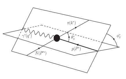
Figure 1: Neutral pion electroproduction in the center of mass frame.

The neutral pion reaction

$$e(l)+p(P)\to e(l^{\prime})+p(P^{\prime})+\pi^{0}(k)$$ (11)

is shown schematically in the virtual photon-proton center of mass frame in Fig. 1. Here, $l=(E_{e},\mathbf{p_{e}})$, $l^{\prime}=(E^{\prime}_{e},\mathbf{p^{\prime}_{e}})$, $P=(m_{p},\mathbf{0})$ and $P^{\prime}=(E^{\prime}_{p},\mathbf{p^{\prime}_{p}})$ are the initial and final electron and proton 4-momenta in the lab frame and $k=(E_{\pi},\mathbf{p_{\pi}})$ is the 4-momentum of the emitted pion. Also, $m_{p}$ refers to the mass of the proton. It is assumed that the incident electron interacts with the target proton via exchange of a single virtual photon with 4-momentum $q=l-l^{\prime}=(\omega,\mathbf{q})$. In this approximation, it is also assumed that the electron mass is negligible ($m_{e}\approx 0$). The two important kinematic invariants of interest are

$$Q^{2}\equiv-q^{2}=-\omega^{2}+|\mathbf{q}|^{2}=4E_{e}E^{\prime}_{e}\sin^{2}(\theta^{\prime}_{e}/2)$$

$$s=W^{2}=(q+P)^{2}=m_{p}^{2}+2\omega m_{p}-Q^{2}.$$ (12)

Here, $\theta^{\prime}_{e}$ is the polar angle of the scattered electron in the lab frame.

The five-fold differential cross section for the reaction can be written in terms of the cross section for the subprocess $\gamma^{*}p\to p\pi^{0}$ Amaldi et al. (1979), which depends only on the matrix elements of the hadronic interaction:

$$\frac{d^{5}\sigma}{dE^{\prime}_{e}d\Omega^{\prime}_{e}d\Omega^{*}_{\pi}}=\Gamma\frac{d^{2}\sigma_{\gamma^{*}p}}{d\Omega^{*}_{\pi}}.$$ (13)

Here, $d\Omega^{\prime}_{e}=d\cos\theta^{\prime}_{e}d\phi^{\prime}_{e}$ is the differential solid angle for the scattered electron in the lab frame and $d\Omega^{*}_{\pi}=d\cos\theta^{*}_{\pi}d\phi^{*}_{\pi}$ is the differential solid angle for the pion in the virtual photon-proton ($\gamma^{*}p$) center of mass frame. The azimuthal angle $\phi^{*}_{\pi}$ is determined with respect to the plane defined by the incident and scattered lepton Drechsel and Tiator (1992). The factor $\Gamma$ represents the virtual photon flux. In the Hand convention Amaldi et al. (1979) it is

$$\Gamma=\frac{\alpha}{2\pi^{2}}\frac{E^{\prime}_{e}}{E_{e}}\frac{W^{2}-m^{2}_{p}}{2m_{p}Q^{2}}\frac{1}{1-\varepsilon},$$ (14)

which depends entirely on the matrix elements of the leptonic interaction and contains the transverse polarization of the virtual photon

$$\varepsilon=\left(1+2\frac{|\mathbf{q}|^{2}}{Q^{2}}\tan^{2}\frac{\theta_{e}^{\prime}}{2}\right)^{-1}.$$ (15)

For unpolarized beam and target the reduced cross section from Eq. (13) can be expanded in terms of the hadronic structure functions:

$$\frac{d\sigma_{\gamma^{*}p}}{d\Omega^{*}_{\pi}} = \frac{|\mathbf{p_{\pi}^{*}}|}{K}\left[\frac{d\sigma_{T}}{d\Omega^{*}_{\pi}}+\varepsilon\frac{d\sigma_{L}}{d\Omega^{*}_{\pi}}+\varepsilon\frac{d\sigma_{TT}}{d\Omega^{*}_{\pi}}\cos 2\phi^{*}_{\pi}\right.$$ (16)

$$+\left.\sqrt{2\varepsilon(\varepsilon+1)}\frac{d\sigma_{LT}}{d\Omega^{*}_{\pi}}\cos\phi^{*}_{\pi}\right].$$

Here, $\mathbf{p_{\pi}^{*}}$ is the pion momentum and $K=(W^{2}-m_{p}^{2})/2W$ is the photon equivalent energy in the c.m. frame of the subprocess $\gamma^{*}p\rightarrow p\pi^{0}$. Additionally, $\sigma_{T}+\varepsilon\sigma_{L}$, $\sigma_{LT}$ and $\sigma_{TT}$ are the structure functions that describe the transverse, longitudinal, longitudinal-transverse interference, and transverse-transverse interference components of the differential cross section.

Each of these structure functions contain the $\cos\theta^{*}_{\pi}$ dependence and can be parameterized in terms of the multipole amplitudes $E_{l\pm}$, $M_{l\pm}$ and $S_{l\pm}$ that describe the electric, magnetic and scalar multipoles, respectively. The scalar multipoles $S_{l\pm}$ can be written in terms of the longitudinal multipoles $L_{l\pm}=\frac{\omega^{*}}{|\mathbf{q^{*}}|}S_{l\pm}$, where $\omega^{*}$ and $\mathbf{q^{*}}$ are the energy and 3-momentum of the virtual photon in the c.m. frame, respectively Drechsel and Tiator (1992).

III Experiment

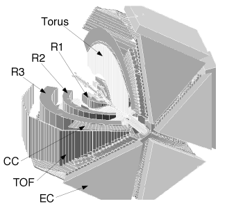
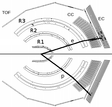
Figure 2: 2 A three-dimensional view of CLAS showing the superconducting coils of the torus, the three regions of drift chambers (R1-R3), the Čerenkov counters, the time-of-flight system, and the electromagnetic calorimeters. The positive ẑ-axis is out of the page along the symmetry axis. 2 A schematic view of a typical near threshold event showing the reconstructed electron and proton tracks with the corresponding detector hits in two opposite CLAS sectors. The $\pi^{0}$ is reconstructed using the missing mass technique as discussed in the text.

The near threshold reaction $ep\to ep\pi^{0}$ was studied using the CEBAF Large Acceptance Spectrometer (CLAS) in Jefferson Lab’s Hall-B Mecking et al. (2003). Fig. 2 shows the detector components that comprise CLAS. Six superconducting coils of the torus divide CLAS into six identical sectors and produce a toroidal magnetic field in the azimuthal direction around the beam axis. Each of the six sectors contain three regions of drift chambers (R1, R2, and R3) to track charged particles and to reconstruct their momentum Mestayer et al. (2000), scintillator counters for identifying particles based on time-of-flight (TOF) information Smith et al. (1999), Čerenkov counters (CC) to identify electrons Adams et al. (2001), and electromagnetic counters (EC) to identify electrons and neutral particles Amarian et al. (2001). The CC and EC are used for triggering on electrons and provide a mechanism to separate charged pions and electrons. With these six sectors, CLAS provides a large solid angle coverage with typical momentum resolutions of about $0.5\%-1.0\%$ depending on the kinematics Mecking et al. (2003).

A 5.754 GeV electron beam with an average intensity of 7 nA was incident on a 5 cm long liquid hydrogen target, which was placed 4 cm upstream of the CLAS center. Fig. 2 shows the electron beam entering CLAS from the top left and exiting from the bottom right through the symmetry axis. A small non-superconducting magnet (minitorus) surrounded the target and generated a toroidal field to shield the R1 drift chambers from low energy electrons of high intensity. These electrons originated primarily from the Møller scattering process. The data used in this experiment were collected from October 2001 to January 2002 and the integrated luminosity was about $0.28$ fb^-1. The electron beam energy of 5.754 GeV as determined in this experiment agrees within 6 MeV with an independent measurement in Hall A Alcorn et al. (2004).

IV Analysis

At the start of this analysis, a cut of $W<1.3$ GeV is applied to focus our events only in the kinematic region of interest. In this analysis the scattered electrons and protons are detected using CLAS and the $\pi^{0}$ is reconstructed using 4-momentum conservation. A typical event for this experiment is shown in Fig. 2.

IV.1 Particle Identification: Electron

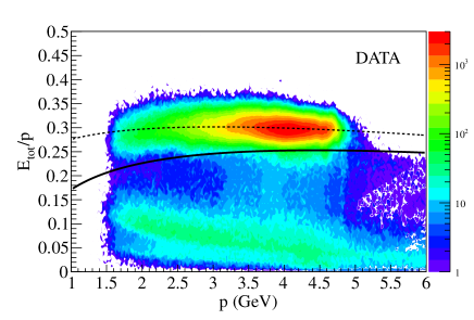
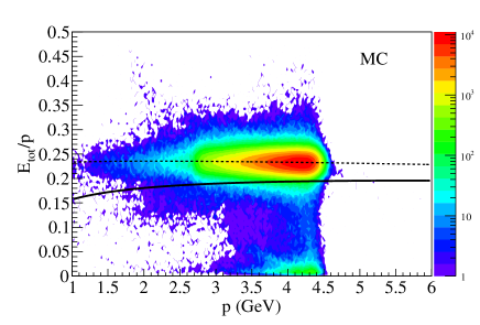
Figure 3: (Color online) EC sampling fraction as a function of electron momentum for one of the CLAS sectors for 3 Data and 3 Monte Carlo (MC) simulation. The dashed lines show the parameterized mean and the solid line indicates the $3\sigma$ cut.

The scattered electrons in the final state of the reaction are detected by requiring geometrical coincidence between the Čerenkov counters and the electromagnetic calorimeter in the same sector. The momentum of the electrons is reconstructed using the drift chambers. Using the energy deposited in the EC and the momentum, the electrons are isolated from most of the minimum ionizing particles (MIPs), e.g., pions, contaminating the electron spectra.

As electrons pass through the EC, they shower with a total energy deposition $E_{tot}$ that is proportional to their momenta $p$. The sampling fraction energy $E_{tot}/p$ is plotted as a function of momentum for each sector after applying all the other electron identification cuts. Fig. 3 shows this distribution for one of the CLAS sectors for experimental and Monte Carlo simulated events. In the figure, one can note the MIPs contamination near the smaller values of $E_{tot}/p$. This contamination is significantly larger in data than in simulated events. The electrons are concentrated near $E_{tot}/p\approx 0.3$. Ideally they should not show any dependence on momentum, albeit a slight momentum dependence is visible in the data. This dependence is parameterized and a cut of $3\sigma$ is applied as shown in the figure. The MIP events are well separated from the electrons below the $3\sigma$ cut.

IV.2 Particle Identification: Proton

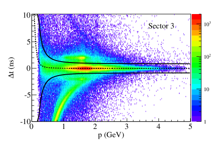
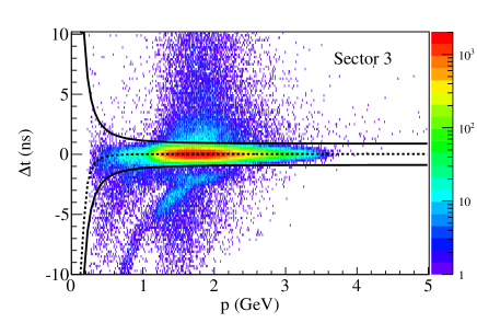
Figure 4: (Color online) $\Delta t$ as a function of $p$. The curves show the $\pm 3.5\sigma$ cut (solid lines) from the mean fit (dashed line) for one of the CLAS sectors for 4 experimental and 4 Monte Carlo simulated events.

The recoiled protons are identified using the measured momentum and the timing information obtained from the TOF counters. A track is selected as a proton whose measured time is closest to that expected of a real proton, i.e.,

$$\Delta t=t_{meas}-t_{calc}=\left(t_{TOF}-t_{tr}\right)-\frac{l}{\beta_{calc}c}.$$ (17)

In the above equation, $t_{TOF}$ is the time measured from the TOF counters, $l$ is the distance from the target center to the TOF paddle, and $t_{tr}$ is the event start time calculated from the electron hit time from the TOF traced back to the target position. Also, in Eq. (17) $\beta_{calc}=p/\sqrt{M^{2}_{pdg}+p^{2}}$, where $\beta_{calc}$ is computed using the PDG Beringer et al. (2012) value of the mass of the proton $M_{pdg}$ and the momentum of the track $p$.

Figs. 4 and 4 show the experimental and simulated event distributions, respectively, of $\Delta t$ as a function of $p$ for one of the CLAS sectors. The protons are centered around $\Delta t=0$ ns and have a slight momentum dependence for $p<1$ GeV. The dashed lines indicate the parameterized mean of the distributions and the solid lines indicate the $\pm 3.5\sigma$ cut applied to select the protons.

IV.3 Fiducial Cuts and Kinematic Corrections

For perfect beam alignment, the incident electron beam is expected to be centered at $(X_{beam},Y_{beam})=(0,0)$ cm at the target. But due to misalignments, the electron beam was actually at $(X_{beam},Y_{beam})=(0.090,-0.345)$ cm. This misalignment of the beam-axis is corrected for each sector, which also subsequently changes the reconstructed $z$-vertex positions of the electron and proton tracks. The details of this correction are described in previous works Ungaro et al. (2006); Park et al. (2008). A cut of $z\in(-8.0,-0.8)$ cm is placed on the $z$-vertex to isolate events from within the target cell.

The measured angles and momenta of the electrons and protons are corrected using the same method as used in previous analyses Ungaro et al. (2006); Park et al. (2008).

The electrons start to lose energy as they enter the electromagnetic calorimeter. When the electrons shower near the edge of the calorimeter, their shower is not fully contained and so their energies cannot be properly reconstructed. As such, a fiducial cut is applied to remove these events.

Electrons give off Čerenkov light in the CC, which is collected in the PMTs on either side of the counters in each sector. Inefficient regions in the CC are isolated by removing those regions where the average number of photo-electrons $\langle Nphe\rangle<5$. This cut results in keeping all events that lie in regions where the CC efficiency is about 99% Adams et al. (2001).

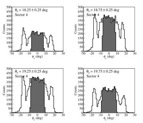
Figure 5: Electron $\phi_{e}$ distribution for CLAS Sector 4 for $p_{e}=4.1\pm 0.1$ GeV shown for different $\theta_{e}$ slices. The unshaded curves show $\phi_{e}$ distribution after electron selection and the shaded curves show the $\phi_{e}$ distribution after applying electron DC fiducial cuts.

To deal with edges and holes in the drift chambers, and to remove dead or inefficient wires, a fiducial cut for both electrons and protons is applied. Regions of non-uniform acceptance in the azimuthal angle $\phi$ resulting from these attributes are isolated on a sector-by-sector basis as a function of the electron’s momentum $p_{e}$ and polar angle $\theta_{e}$. For the electron, at fixed $p_{e}$ and $\theta_{e}$, one expects the angular distribution to be symmetric in $\phi_{e}$ and relatively flat. Empirical cuts are applied to select these regions of relatively flat $\phi_{e}$ as shown in Fig. 5 for electrons with $p=4.1\pm 0.1$ GeV for different slices of $\theta_{e}$ and one of the CLAS sectors. The same cuts are applied to both experimental and simulated events.

As for electrons, a fiducial cut on the proton’s azimuthal angle $\phi_{p}$ as a function of its momentum $p_{p}$ and polar angle $\theta_{p}$ is applied. However, the edges of the $\phi_{p}$ distributions are asymmetric for different slices of $\theta_{p}$. The upper and lower bounds on $\phi_{p}$ are extracted and parameterized as a function of $\theta_{p}$ and $p_{p}$. The result of this cut for one of the CLAS sectors is shown in Fig. 6.

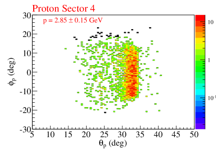
Figure 6: (Color online) Proton $\phi_{p}$ vs. $\theta_{p}$ distribution for CLAS Sector 4 for $p_{p}=2.85\pm 0.15$ GeV. Rejected tracks are shown in black.

IV.4 Background Subtraction and $\pi^{0}$ Identification

The neutral pion in the final state is reconstructed using energy and momentum conservation constraint. To do so, we use the conservation of 4-momentum and look at the missing mass squared distribution of the detected particles (i.e., the electron and the proton):

$$M_{X}^{2}(ep)=(l+P-l^{\prime}-P^{\prime})^{2}.$$ (18)

Here, $l$, $P$, $l^{\prime}$ and $P^{\prime}$ are 4-momenta of the incident and scattered particles as described in Section II.

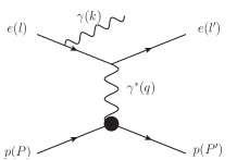
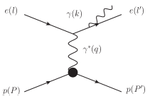
Figure 7: The Bethe-Heitler process $ep\to ep\gamma$ diagrams for 7 a photon emitted from an incident electron (pre-radiation) and for 7 a photon emitted from a scattered electron (post-radiation).

There are several difficulties in the analysis in the near threshold region. In this region, the pion electroproduction cross section goes to zero; so, the statistics are very low. Also, a major source of contamination to the neutral pion signal near threshold is the elastic Bethe-Heitler process $ep\to ep\gamma$. The two dominating Feynman diagrams for this process are shown in Fig. 7. Fig. 7 shows the diagram with a pre-radiated photon (emission from an incident electron) and Fig. 7 shows the diagram with a post-radiated photon (emission from a scattered electron). These photons are emitted approximately in the direction of the incident and scattered electron, respectively Schiff (1952); Ent et al. (2001). When these photons are emitted, the incident and scattered electrons lose energy. This feature of the Bethe-Heitler process can be exploited to our benefit.

For the elastic process $ep\to ep$, the proton angle can be computed independently of the incident or scattered electron energies:

$$\tan\theta^{p}_{1} = \frac{1}{\left(1+\frac{E^{\prime}}{m_{p}-E^{\prime}\cos\theta_{e}^{\prime}}\right)\tan\frac{\theta_{e}^{\prime}}{2}}$$ (19)

$$\tan\theta^{p}_{2} = \frac{1}{\left(1+\frac{E}{m_{p}}\right)\tan\frac{\theta_{e}^{\prime}}{2}}.$$ (20)

Here, $\theta^{p}_{1}$ and $\theta^{p}_{2}$ are the proton angles computed independently of the incident or scattered electron energies, respectively. Also, $\theta_{e}^{\prime}$ is the angle of the scattered electron in the lab frame, and $E$ and $E^{\prime}$ are the energies of the incident and scattered electron, respectively. We can calculate these angles for each event and look at its deviation ($\Delta\theta_{1,2}^{p}$) from the measured value ($\theta^{p}_{meas}$):

$$\Delta\theta_{1,2}^{p}\equiv\theta_{1,2}^{p}-\theta^{p}_{meas}.$$ (21)

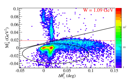
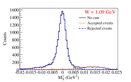
Figure 8: (Color online) 8 $M_{X}^{2}$ vs $\Delta\theta_{1}^{p}$ for $W=1.09\pm 0.01$ GeV. The red dashed line indicates the expected pion peak position. The left red spot centered around zero degrees corresponds to the elastic scattering events in which the incident electrons have undergone Bethe-Heitler radiation (pre-radiative) and the one on the right to the elastic post-radiative events. The events below the linear polynomial and outside the ellipse are selected as pions. 8 $M_{X}^{2}$ for events with $W=1.09\pm 0.01$ GeV. The black solid curve shows events prior to any Bethe-Heitler subtraction cuts, the blue dashed-dot curve shows events rejected from the cuts, and the red dashed curve shows those events that survive the Bethe-Heitler subtraction cuts.

Fig. 8 shows the $M_{X}^{2}$ plotted as a function of this deviation $\Delta\theta_{1}^{p}$ for one of the near threshold regions, $W=1.09\pm 0.01$ GeV. In the plot, we see two red spots along $M_{X}^{2}=0\,\textrm{GeV}^{2}$. The one on the left is centered along $\Delta\theta_{1}^{p}=0$ deg corresponding to the pre-radiated photon events. The other corresponds to the post-radiated photon events. Additionally, these radiative events are also present in the positive $M_{X}^{2}$. These are the radiative events that we need to isolate from the pion signal as indicated by the red dashed line in the plot. An ellipse and a linear polynomial are used to reject these events. These cuts are parameterized as a function of $W$. The result of these cuts is seen in Fig. 8 with the accepted events after the cut shown in red (dashed curve) as our pions and the rejected events in blue (dashed-dot curve).

After the Bethe-Heitler subtraction cuts are applied, the pions are selected by making a $\pm 3\sigma$ cut on $M_{X}^{2}$ from the mean position of the distribution. An example of the distributions and fit are shown in Fig. 9. The $M_{X}^{2}$ distributions (black circles) are fit with two Gaussians. The blue (dashed-dot) curve is an estimate of the remaining Bethe-Heitler background in the $M_{X}^{2}$ distribution, which was not eliminated by the elliptical cuts of Fig. 8. This was subtracted to yield the green (triangle) points. A systematic uncertainty of $\pm 8\%$ is associated with this background subtraction procedure, which is detailed in Sec. VII.

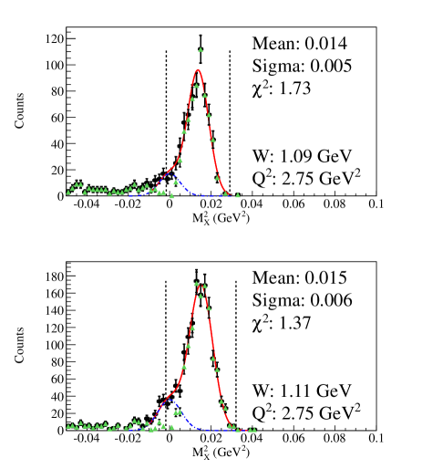
Figure 9: (Color online) An example of the $M_{X}^{2}(ep)$ distribution with a double Gaussian fit after applying the elliptical cuts (black circles) of Fig. 8 and after residual Bethe-Heitler and other contamination subtractions (green triangles) for $Q^{2}=2.75\pm 0.25$ GeV² and $W=1.09\pm 0.01$ GeV (top) and $W=1.11\pm 0.01$ GeV (bottom) integrated over all $\phi^{*}_{\pi}$ and $\cos\theta^{*}_{\pi}$. The black dashed lines indicate the $\pm 3\sigma$ cuts applied to select the pions. The $\chi^{2}$ is the goodness of fit per degree of freedom. See Sec. IV.4 for details.

V Simulations

To determine the cross section, a Monte Carlo simulation study is required, including a physics event generator and the detector geometry. Events are generated using the MAID2007 unitary isobar model (UIM) Drechsel et al. (2007), which uses a phenomenological fit to previous photo- and electroproduction data. Nucleon resonances are described using Breit-Wigner forms and the non-resonant backgrounds are modeled from Born terms and $t$-channel vector-meson exchange. To describe the threshold behavior, Born terms were included with mixed pseudovector-pseudoscalar $\pi NN$ coupling Drechsel et al. (2007). While the pion electroproduction world-data in the resonance region goes up to $Q^{2}\sim 7$ GeV² Villano et al. (2009) for $W>1.11$ GeV, there are no data near threshold for $Q^{2}>2$ GeV² and $W<1.11$ GeV (the kinematics of this work). Thus, cross sections for the kinematics of this work are described by extrapolations of the fits to the existing data in the MAID2007 model.

Events are generated to cover the entire kinematic range described in Table 1. About 73 million events are generated for the 2400 kinematic bins and 6.7 million events were reconstructed after all analysis cuts. The average resolutions of the kinematic quantities, $W$, $Q^{2}$, $\cos\theta_{\pi}^{*}$, and $\phi_{\pi}^{*}$ are 0.014 GeV, 0.008 GeV², 0.05, and 8 degrees, respectively. These resolutions are obtained by comparing the generated kinematic quantities with those after reconstruction.

Variable	Range	Number of Bins	Width
$W$ (GeV)	1.08 : 1.16	4	0.02
$Q^{2}$ (GeV2)	2.0 : 4.5	4	variable
$\cos\theta_{\pi}^{*}$	-1 : 1	5	0.4
$\phi_{\pi}^{*}$ (deg)	0 : 360	6	60

Table 1: Kinematic bin selection.

After the physics events are generated, their passage through the detector is simulated using the GEANT3 based Monte Carlo (GSIM) program. This program simulates the geometry of the CLAS detector during the experiment and the interaction of the particles with the detector material. GSIM models the effects of multiple scattering of particles in the CLAS detector and geometric mis-alignments. The information for all interactions with the detectors is recorded in raw banks, which is used for reconstruction of the tracks.

The events from GSIM are fed through a program called the GSIM Post Processor (GPP) to incorporate effects of tracking resolution and dead wires in the drift chambers, and timing resolutions of the TOF.

These events are then processed using the same codes as those events from the experiment to reconstruct tracks and higher level information such as 4-momentum, timing, and so on. The simulated events are analyzed the same way as the experimental data and are used to obtain acceptance corrections and radiative corrections for the cross sections calculations.

VI Corrections

VI.1 Acceptance Corrections

Acceptance corrections are applied to the experimental data to obtain the cross section for each kinematic bin. These corrections describe the geometrical coverage of the CLAS detector, inefficiencies in hardware and software, and resolution effects from track reconstruction.

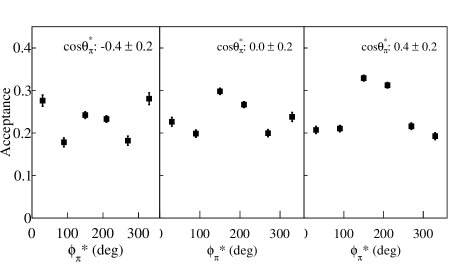
Figure 10: Acceptance corrections for $W=1.09$ GeV and $Q^{2}=2.75$ GeV² as a function of $\phi_{\pi}^{*}$. Each subplot shows the correction for a different $\cos\theta_{\pi}^{*}$ bin.

By comparing the number of events in each kinematic bin from the physics generator and the reconstruction process, the acceptance can be obtained as:

$$A_{i}=\frac{N^{i}_{rec}}{N^{i}_{gen}},$$ (22)

where $N^{i}_{rec}$ corresponds to those events that have gone through the entire analysis process including track reconstruction and all analysis cuts. $N^{i}_{gen}$ are those events that were generated. Fig. 10 shows the acceptances for a few of the near threshold bins as a function of $\phi_{\pi}^{*}$.

VI.2 Radiative Corrections

The radiative correction is obtained using the software package EXCLURAD Afanasev et al. (2002) that takes theoretical models as input to compute the corrections. For this experiment the MAID2007 model, the same model used to generate Monte Carlo events, is used to determine the radiative corrections. The radiative corrections are closely related to the acceptance corrections. For each kinematic bin the differential cross section can be written as:

$$\sigma=\frac{N_{meas}}{\mathcal{L}\,A}\frac{1}{\delta},$$ (23)

where $N_{meas}/\mathcal{L}$ is the number of events from the experiment normalized by the integrated luminosity (with appropriate factors) before acceptance and radiative corrections. Also, $A=N^{RAD}_{rec}/N^{RAD}_{gen}$ is the acceptance correction for the bin and $\delta$ is the radiative correction. It should be noted that the events for the acceptance correction were generated with a radiated photon in the final state using the MAID2007 model.

EXCLURAD uses the same model to obtain the correction $\delta=N^{RAD^{\prime}}_{gen}/N^{NORAD^{\prime}}_{gen}$, where $N^{NORAD^{\prime}}_{gen}$ are events generated without a radiated photon in the final state. Thus

$$\sigma=\frac{N_{meas}}{\mathcal{L}}\left(\frac{N^{RAD}_{gen}}{N^{RAD}_{rec}}\right)\times\left(\frac{N^{NORAD^{\prime}}_{gen}}{N^{RAD^{\prime}}_{gen}}\right).$$ (24)

The details of the radiative correction procedure are described in Ref. Park et al. (2008).

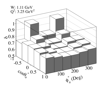
Figure 11: The radiative corrections for $W=1.11$ GeV and $Q^{2}=3.25$ GeV² as a function of $\cos\theta_{\pi}^{*}$ and $\phi^{*}_{\pi}$ obtained from EXCLURAD using the MAID2007 model.

Fig. 11 shows the radiative corrections calculated for one of the kinematic bins as a function of the pion angles in the c.m. system. One can observe that the corrections have a $\phi^{*}_{\pi}$ dependence. This is because the bremsstrahlung process only occurs near the leptonic plane, $i.e.$, at angles near 0 or 180 degrees with respect to the hadronic plane. Also, one can notice that the correction increases with $\cos\theta_{\pi}^{*}\to-1$. This is because the cross section is expected to approach zero at backwards angles and that is the region where the Bethe-Heitler events dominate. The average radiative correction over all kinematic bins is $\sim 25\%$.

VI.3 Other Corrections

Two other corrections were applied to the cross section. One of them involves estimating the fraction of the events originating from the target cell walls and the other is an empirical overall normalization factor.

To estimate the level of contamination from the target cell walls, events collected during the empty-target run period of the experiment are analyzed using the same process as those for the production run period. Only those events that fall within the target wall region for the empty target should be considered for the source of contamination. This is because even though there was no liquid hydrogen in the target, it was still filled with cold hydrogen gas. So, for this estimation only events within $\pm 0.5$ cm of the target wall region are selected. The correction is then calculated by taking the ratio of events within this target region from the empty target runs to those from the production run normalized to the total charge, $\rho$, collected during the run periods,

$$R=\frac{N_{\mathrm{empty\,target}}}{N_{\mathrm{production}}}\frac{\rho_{\mathrm{production}}}{\rho_{\mathrm{empty\,target}}}.$$ (25)

The average contamination is approximately $1\%-1.9\%$ depending on the $W$ kinematic bin. This ratio is then applied as a correction factor to the measured cross section $\sigma=\sigma_{meas}(1-R)$. Here, $\sigma$ is the corrected cross section and $\sigma_{meas}$ is the measured cross section for a particular bin in $W$.

The second correction (the empirical overall normalization factor) comes from comparing the measured $ep\to ep$ elastic and the $ep\to ep\pi^{0}$ cross sections in the $\Delta(1232)$ resonance region ($W=1.23$ GeV) to previously measured values Bosted (1995); Ungaro et al. (2006); Aznauryan et al. (2009); Drechsel et al. (2007). The measured elastic scattering cross section from this experimental data were compared to the known cross section values Bosted (1995) where both the electron and the proton were detected in the final state. A deviation of $\sim 11\%$ from the known cross section values is observed.

This deviation of $\sim 11\%$ from the known elastic electron-proton scattering cross section includes the inefficiencies associated with the proton detection in CLAS Mecking et al. (2003); Bedlinskiy et al. (2012).

To account for this discrepancy, an overall normalization factor of $R_{elastic}=0.89$ is applied to the $ep\to ep\pi^{0}$ differential cross section for every kinematic bin. An associated systematic uncertainty of $\pm 5\%$ is applied. After this correction is applied, the measured $ep\to ep\pi^{0}$ cross sections for the $\Delta(1232)$ resonance region, $W=1.23\pm 0.01$ GeV, are in agreement with previous measurements Ungaro et al. (2006); Aznauryan et al. (2009); Drechsel et al. (2007) to within $5\%$ on average. Fig. 12 shows the result of this correction for a few kinematic bins in the $\Delta(1232)$ resonance region.

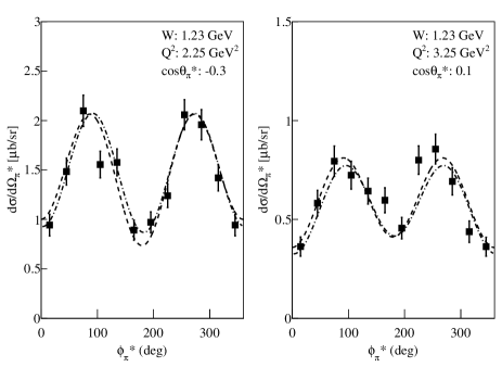
Figure 12: The differential cross section $ep\to ep\pi^{0}$ for the $\Delta(1232)$ resonance region, $W=1.23\pm 0.01$ GeV, for typical kinematic bins. The squares are the measured cross sections after applying the normalization correction factor (see text for details). The dashed curves are from Ref. Aznauryan et al. (2009) and the dashed-dot curves are from the MAID2007 model. The corrected values agree with the two curves to within $5\%$ on average.

Since the threshold region of interest for this experiment is sandwiched between the elastic and the $\Delta(1232)$ resonance region and the results in these two regions are consistent with previous measurements after applying this overall normalization factor, we believe this procedure is justified. This correction to the cross section also includes any detector inefficiencies and, as such, these inefficiencies will not be accounted for separately.

VII Systematic Studies

To determine the systematic uncertainties in the analysis, the parameters of the likely sources of those uncertainties are varied within reasonable bounds and the sensitivity of the final result is checked against this variation. A summary of the systematic uncertainties averaged over the kinematic bins of interest is shown in Table 2.

The electron and proton identification cuts, the electron fiducial cuts, the vertex cuts and the target cell correction cuts provide small contributions to the overall systematic uncertainties.

The electron EC sampling fraction cuts were varied from $3\sigma$ to $3.5\sigma$ and the extracted structure functions changed by about $0.4\%$ on average. The parameters for the electron fiducial cuts were similarly varied by about $10\%$ and the structure functions changed by about $1\%$ on average. As such, a systematic uncertainty of $0.4\%$ and $1\%$ was assigned to these sources.

The $\Delta t$ cuts to select the protons were varied from $3.5\sigma$ to $4\sigma$ and a variation of about $1.1\%$ on average was observed on the extracted structure functions, which was assigned as the systematic uncertainty associated with this source. The variations in the fiducial cuts for the proton had a negligible effect on the structure functions.

The vertex cuts were reduced by $5\%$ and a variation of about $0.1\%$ on average was observed on the extracted structure functions. So, a systematic uncertainty of $0.1\%$ was assigned to this source. The structure functions are compared before and after applying the target cell corrections. A variation of about $1\%$ is observed and this value was assigned as a source of systematic uncertainty.

The major sources of systematic uncertainty are the Bethe-Heitler background subtraction, the missing mass squared cut to select the neutral pions, the elastic normalization corrections and the model dependence of the acceptance and radiative corrections.

There are residual Bethe-Heitler events that escape the elliptical Bethe-Heitler cuts. These events peak at $M_{X}^{2}=0$, which have to be included in the overall fit. A Gaussian distribution was assumed for both the $\pi^{0}$ and the remaining Bethe-Heitler events. The pions are modeled by a Gaussian distribution near the expected pion mass and the Bethe-Heitler events are modeled by a Gaussian whose peak is at $M_{X}^{2}=0$. This accounts for much of the tail in Figs. 8 and 9. The resolution for $M_{X}^{2}$ for the Bethe-Heitler and the pion distributions is expected to be similar because of the same kinematics of the detected electron and the proton. The Gaussian fit for the Bethe-Heitler is obtained, which is then subtracted to yield the pions.

To see the effect of the background subtraction, the structure functions were compared with and without the application of the Bethe-Heitler background subtraction cuts. The structure functions changed by about $8\%$ on average and this was used as a systematic uncertainty for this procedure.

The missing mass squared cut was varied from $3\sigma$ to $4\sigma$ and this resulted in a change of about $3\%$ on average in the extracted structure functions.

The systematic uncertainty on the elastic normalization correction of $\pm 5\%$ was obtained by looking at the difference between the extracted structure functions before and after applying the correction factor to the data. The structure functions varied by about $5\%$ on average.

Additionally, a $\pm 4\%$ systematic uncertainty is assigned on the model dependence of the acceptance and radiative corrections based on previous analyses Ungaro et al. (2006); Park et al. (2008, 2012).

The total average systematic uncertainty, obtained by adding the individual contributions in quadrature is 10.8%.

Source	Estimate %
$e^{-}$ EC sampling fraction cuts	0.4
$e^{-}$ fiducial cuts	1
$p$ $\Delta t$ cuts	1.1
Vertex cuts	0.1
Background subtraction cuts	8
$\pi^{0}$ $M_{X}^{2}$ cut	3
Target cell correction	1
Elastic normalization correction	5
Acceptance and radiative correction	4
Total	10.8

Table 2: The average systematic uncertainties for the differential cross sections from various sources and the corresponding criteria. The final quoted systematic uncertainty, obtained by adding the different systematic uncertainties from each source in quadrature, is about 10.8%.

VIII Differential Cross Sections and Structure Functions

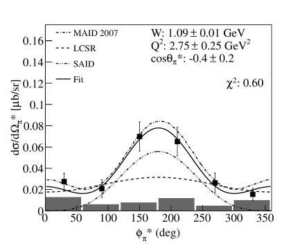
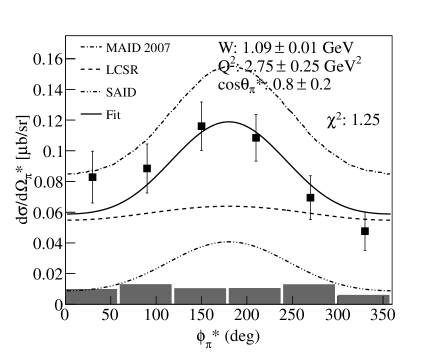
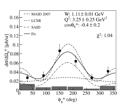
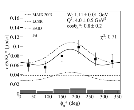
Figure 13: The differential cross sections in $\mu$b/sr for a few kinematic bins near threshold as a function of $\phi_{\pi}^{*}$. Experimental points (squares) are shown with statistical uncertainties only. The size of the estimated systematic uncertainties is shown in gray boxes below. The predictions from LCSR, MAID2007 and SAID are shown as dashed, dashed-dotted and dashed-double-dotted curves, respectively. The fit to the distributions is shown as a solid curve. See Sec. VIII for details.

The kinematic coverage of the experiment spans over $W$ from $1.08$ to $1.16$ GeV and $Q^{2}$ from $2$ to $4.5$ GeV². The reduced differential cross section for the reaction is computed for each kinematic bin. The cross sections are reported at the center of each kinematic bin. Fig. 13 shows the differential cross section for some of the kinematic bins near threshold as a function of $\phi_{\pi}^{*}$. The predictions from LCSR Braun et al. (2008), MAID2007 Drechsel et al. (2007) and SAID Arndt et al. (2009) are shown for comparison.

Using Eq. (16), the differential cross section is fitted to extract the structure functions $\sigma_{T}+\varepsilon\sigma_{L}$, $\sigma_{TT}$ and $\sigma_{LT}$. The result of the fit is shown as the solid curve in Fig. 13. The reduced $\chi^{2}$ for the fit is calculated using $\chi^{2}=\chi_{0}^{2}/\nu$, where $\nu$ is the number of degrees of freedom calculated for each $W$, $Q^{2}$, and $\cos\theta_{\pi}^{*}$ bin (i.e., $\nu=6$ data points $-3$ fit parameters $=3$), and $\chi_{0}^{2}$ is the unnormalized goodness of fit. The averaged $\chi^{2}$ of the fits is 0.9.

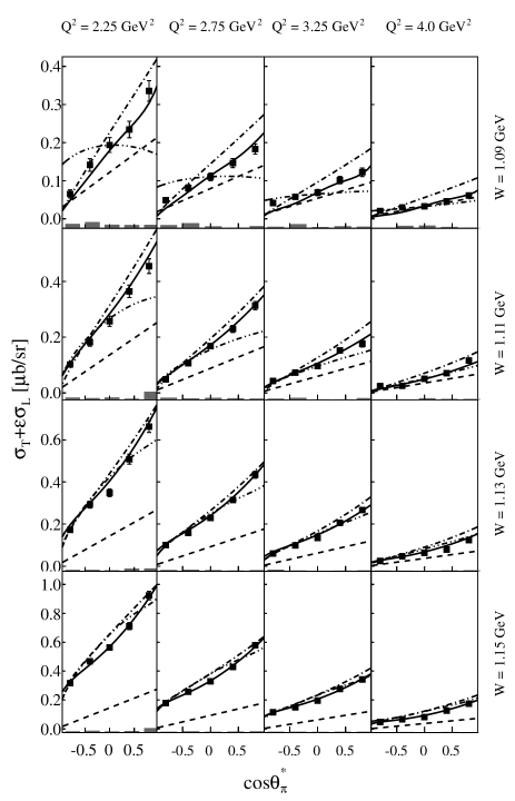
Figure 14: The structure function $\sigma_{T}+\varepsilon\sigma_{L}$ as a function of $\cos\theta_{\pi}^{*}$ in $\mu$b/sr for $W=1.08-1.16$ GeV and $Q^{2}=2.0-4.5$ GeV². Predictions from LCSR that include only $s$-wave contribution (dashed), MAID2007 (dashed-dot), and SAID (dashed-double-dot) are shown. The error bars represent statistical uncertainties only and the estimated systematic uncertainties are shown as gray boxes. The solid curve corresponds to the results obtained from the fit to the cross sections (see Sec. IX for details). The values of $Q^{2}$ (on top of the panels) and $W$ (on the right side of the panels) are the central values of the bins.

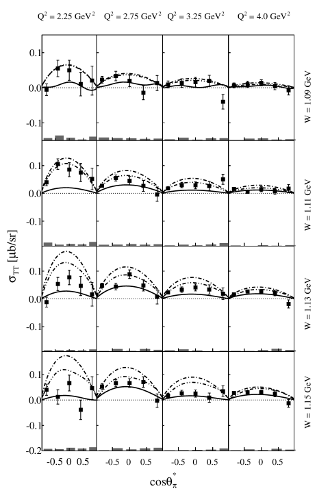
Figure 15: The structure function $\sigma_{TT}$ as a function of $\cos\theta_{\pi}^{*}$ in $\mu$b/sr for $W=1.08-1.16$ GeV and $Q^{2}=2.0-4.5$ GeV². Predictions from MAID2007 (dashed-dot) and SAID (dashed-double-dot) are shown. The LCSR predictions do not include any $\sigma_{TT}$ contributions, so they are not shown. The error bars represent statistical uncertainties only and the estimated systematic uncertainties are shown as gray boxes. The solid curve corresponds to the results obtained from the fit to the cross sections (see Sec. IX for details). The values of $Q^{2}$ (on top of the panels) and $W$ (on the right side of the panels) are the central values of the bins. The horizontal line at zero serves as a visual aid.

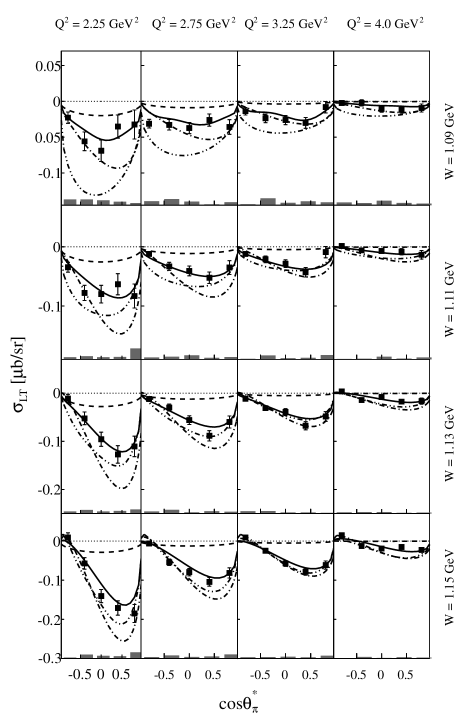
Figure 16: The structure function $\sigma_{LT}$ as a function of $\cos\theta_{\pi}^{*}$ in $\mu$b/sr for $W=1.08-1.16$ GeV and $Q^{2}=2.0-4.5$ GeV². Predictions from LCSR that include only $s$-wave contribution (dashed), MAID2007 (dashed-dot), and SAID (dashed-double-dot) are shown. The error bars represent statistical uncertainties only and the estimated systematic uncertainties are shown as gray boxes. The solid curve corresponds to the results obtained from the fit to the cross sections (see Sec. IX for details). The values of $Q^{2}$ (on top of the panels) and $W$ (on the right side of the panels) are the central values of the bins. The horizontal line at zero serves as a visual aid.

The extracted structure functions $\sigma_{T}+\varepsilon\sigma_{L}$, $\sigma_{TT}$ and $\sigma_{LT}$ are shown in Figs. 14, 15 and 16, respectively, as a function of $\cos\theta_{\pi}^{*}$ for $W=1.08-1.16$ GeV and $Q^{2}=2.0-4.5$ GeV². The data points are shown with statistical error bars only and the size of the systematic errors is shown as the gray boxes. Predictions from LCSR, MAID2007, and SAID are also included for $\sigma_{T}+\varepsilon\sigma_{L}$ and $\sigma_{LT}$. Since the LCSR does not include any $\sigma_{TT}$ contributions in the calculations, they are not shown.

The structure function $\sigma_{T}+\varepsilon\sigma_{L}$ (Fig. 14) is generally in good agreement with the MAID2007 predictions but there is some discrepancy for $W=1.09$ GeV at high $\cos\theta_{\pi}^{*}$. This discrepancy is reduced for higher $W$ bins. The results disagree with the LCSR predictions, especially for those bins away from threshold ($W>1.09$ GeV). This disagreement is also apparent for low $Q^{2}$ bins. As one moves closer to threshold and at high $Q^{2}$, the agreement is quite good, especially at backward angles $\cos\theta_{\pi}^{*}\to-1$. The LCSRs have been calculated and tuned especially for the threshold region at high $Q^{2}$ and thus, there exists a strong disagreement at higher $W$ and low $Q^{2}$ bins. The predictions from SAID strongly disagree for the first $W$ bin and low $Q^{2}$ bins, but converge toward the MAID2007 predictions for higher $W$ and $Q^{2}$.

The structure function $\sigma_{TT}$ (Fig. 15) results are in good agreement with the SAID and MAID2007 predictions for low $W$ and high $Q^{2}$ but disagree at high $W$ and low $Q^{2}$ bins. Most of the values are close to zero for all $W$. The LCSR predictions assume only $s$-wave contributions to the cross section from this structure function. The $d$-wave contribution to the total cross sections in SAID range from $0$ to $0.001$ $\mu$b for the near threshold bins Arndt et al. (2009).

The structure function $\sigma_{LT}$ (Fig. 16) also shows good agreement with the MAID2007 and LCSR predictions for high $Q^{2}$ and low $W$, but there is some discrepancy at other kinematics. The SAID prediction has a large disagreement at low $W$ and $Q^{2}$, but the level of agreement at other kinematics is similar to the MAID2007 model.

IX $S$-Wave Multipoles and Generalized Form Factors

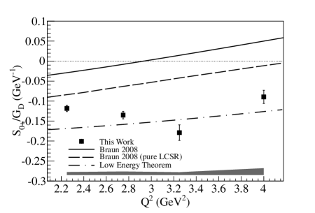
Figure 17: The $s$-wave multipoles 17 $E_{0+}$ and 17 $S_{0+}$ normalized to the dipole formula $G_{D}$ are plotted as a function of $Q^{2}$. The error bars include statistical and systematic uncertainties added in quadrature. The size of the estimated systematic uncertainties are shown in the bottom. The LCSR based model predictions and the LET predictions are also shown as curves. The horizontal line at zero serves as a visual aid.

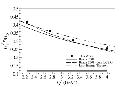
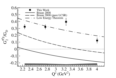
Figure 18: The generalized form factors 18 $G_{1}^{\pi^{0}p}$ and 18 $G_{2}^{\pi^{0}p}$ normalized to the dipole formula $G_{D}$ are plotted as a function of $Q^{2}$. The error bars include statistical and systematic uncertainties added in quadrature. The size of the estimated systematic uncertainties are shown in the bottom. The LCSR based model predictions and the LET predictions are also shown as curves. The horizontal line at zero serves as a visual aid.

In order to compare with the calculated generalized form factors of Ref. Braun et al. (2008), one must extract the $s$-wave multipole amplitudes from the measured cross sections. First, the structure functions are written in terms of the helicity amplitudes $H_{i}$. The helicity amplitudes are functions defined by transitions between eigenstates of the helicities of the nucleon and the virtual photon Amaldi et al. (1979). The helicity amplitudes are then expanded in terms of the multipole amplitudes.

The structure functions are related to the helicity amplitudes $H_{1,2,...6}(W,Q^{2},\cos\theta_{\pi}^{*})$ by:

$$\sigma_{T} = \frac{1}{2}(|H_{1}|^{2}+|H_{2}|^{2}+|H_{3}|^{2}+|H_{4}|^{2}),$$ (26)

$$\sigma_{L} = |H_{5}|^{2}+|H_{6}|^{2},$$ (27)

$$\sigma_{TT} = Re(H_{3}H_{2}^{*}-H_{4}H_{1}^{*}),$$ (28)

$$\sigma_{LT} = -\frac{1}{\sqrt{2}}Re[(H_{1}-H_{4})H_{5}^{*}+(H_{2}+H_{3})H_{6}^{*}].$$ (29)

The analysis of the data is based on the following expansion of the helicity amplitudes over multipole amplitudes (see, for example, Aznauryan and Burkert (2012)):

$$H_{1} = \frac{1}{\sqrt{2}}\sin\theta^{*}_{\pi}\cos\frac{\theta^{*}_{\pi}}{2}\sum(B_{l+}-B_{(l+1)-})$$ (30)

$$[P^{\prime\prime}_{l}(\cos\theta^{*}_{\pi})-P^{\prime\prime}_{l+1}(\cos\theta^{*}_{\pi})],$$

$$H_{2} = \sqrt{2}\cos\frac{\theta^{*}_{\pi}}{2}\sum(A_{l+}-A_{(l+1)-})$$ (31)

$$[P^{\prime}_{l}(\cos\theta^{*}_{\pi})-P^{\prime}_{l+1}(\cos\theta^{*}_{\pi})],$$

$$H_{3} = \frac{1}{\sqrt{2}}\sin\theta^{*}_{\pi}\sin\frac{\theta^{*}_{\pi}}{2}\sum(B_{l+}+B_{(l+1)-})$$ (32)

$$[P^{\prime\prime}_{l}(\cos\theta^{*}_{\pi})+P^{\prime\prime}_{l+1}(\cos\theta^{*}_{\pi})],$$

$$H_{4} = \sqrt{2}\sin\frac{\theta^{*}_{\pi}}{2}\sum(A_{l+}+A_{(l+1)-})$$ (33)

$$[P^{\prime}_{l}(\cos\theta^{*}_{\pi})+P^{\prime}_{l+1}(\cos\theta^{*}_{\pi})],$$

$$H_{5} = \frac{Q}{|\mathbf{q^{*}}|}\cos\frac{\theta^{*}_{\pi}}{2}\sum(l+1)(S_{l+}+S_{(l+1)-})$$ (34)

$$[P^{\prime}_{l}(\cos\theta^{*}_{\pi})-P^{\prime}_{l+1}(\cos\theta^{*}_{\pi})],$$

$$H_{6} = \frac{Q}{|\mathbf{q^{*}}|}\sin\frac{\theta^{*}_{\pi}}{2}\sum(l+1)(S_{l+}-S_{(l+1)-})$$ (35)

$$[P^{\prime}_{l}(\cos\theta^{*}_{\pi})+P^{\prime}_{l+1}(\cos\theta^{*}_{\pi})].$$

Here, $P^{\prime}_{l,l+1}(\cos\theta_{\pi}^{*})$ and $P^{\prime\prime}_{l,l+1}(\cos\theta_{\pi}^{*})$ are the first and second derivatives of the Legendre polynomials, respectively, and $\mathbf{q^{*}}$ is the virtual photon 3-momentum in the c.m. system. Also,

$$A_{l+} = \frac{1}{2}\left[(l+2)E_{l+}+lM_{l+}\right],$$ (36)

$$B_{l+} = E_{l+}-M_{l+},$$ (37)

$$A_{(l+1)-} = \frac{1}{2}\left[(l+2)M_{(l+1)-}-lE_{(l+1)-}\right],$$ (38)

$$B_{(l+1)-} = E_{(l+1)-}+M_{(l+1)-}.$$ (39)

The strong $\cos\theta^{*}_{\pi}$-dependence of the structure function $\sigma_{T}+\varepsilon\sigma_{L}$ and the nonzero values of $\sigma_{LT}$ found in the experiment (see Figs. 14 and 16) show that higher multipole amplitudes should be taken into account in addition to the $s$-wave amplitudes $E_{0+}$ and $S_{0+}$ at all $W$. Our understanding of the high-wave multipoles, which should be included in this analysis, was based on the results of the analysis of CLAS data Ungaro et al. (2006); Park et al. (2008) performed in Ref. Aznauryan et al. (2009) using the unitary isobar model (UIM) and dispersion relations (DR). These data are on the $\gamma^{*}p\rightarrow\pi^{+}n$ Park et al. (2008) and $\gamma^{*}p\rightarrow\pi^{0}p$ Ungaro et al. (2006) cross sections in a similar range of $Q^{2}$ but in a significantly wider energy range, which start from $W=$ 1.15 and 1.11 GeV, respectively. The precision in the present experimental results near threshold is much better than the precision in Refs. Ungaro et al. (2006); Park et al. (2008). However, the results of their analysis are useful to study the $p$- and $d$-wave contributions, which are determined mainly by the $\Delta(1232)P_{33}$, $N(1440)P_{11}$, and $N(1520)D_{13}$ resonances.

According to the results of the analysis Aznauryan et al. (2009) at $W=1.09$ to $1.15$ GeV, there are large $p$-wave contributions related to the $\Delta(1232)P_{33}$ and $N(1440)P_{11}$. The $d$-wave contributions are negligibly small for the following reasons: (i) near threshold, the $d$-wave multipole amplitudes are suppressed compared to the $p$-wave amplitudes by the additional kinematical factor $p^{*}_{\pi}$; (ii) at the values of $Q^{2}$ investigated in this experiment, the contribution of the $N(1520)D_{13}$ to the corresponding multipole amplitudes is significantly smaller than the contributions of the $\Delta(1232)P_{33}$ and $N(1440)P_{11}$ to the $p$-wave multipole amplitudes; (iii) in contrast with the $\Delta(1232)P_{33}$ and $N(1440)P_{11}$, the width of the $N(1520)D_{13}$ is significantly smaller than the difference between the mass of the resonance and total energy at the threshold. Therefore, in our analysis only multipole amplitudes $E_{0+}$, $S_{0+}$, $M_{1\pm}$, $S_{1\pm}$, and $E_{1+}$ were included.

The data were fitted simultaneously at $W=$ 1.09, 1.11, 1.13 and 1.15 GeV with statistical and systematic uncertainties added in quadrature for each point. The amplitudes were parametrized according to their threshold behavior and the results of the analysis in Ref. Aznauryan et al. (2009).

Due to the Watson theorem Watson (1954), the imaginary parts of the multipole amplitudes below the $2\pi$ production threshold are related to their real parts as $Im\mathcal{M}=Re\mathcal{M}\tan(\delta_{\pi N}^{I})$, where $\mathcal{M}$ denotes $E^{I}_{l\pm}$, $M^{I}_{l\pm}$ or $S^{I}_{l\pm}$ amplitudes, and $I$ is the total isotopic spin of the $\pi N$ system. Near threshold $\delta^{I}_{\pi N}\sim p_{\pi}^{*2l+1}$, and the imaginary parts of the multipole amplitudes are suppressed compared to their real parts. Therefore, in the analysis, only the real parts of the amplitudes were kept. These amplitudes were parameterized as follows: $E_{0+},S_{0+}\sim const$, $M_{1\pm}$, $S_{1\pm}$, and $E_{1+}\sim p^{*}_{\pi}$.

In the fitting procedure, the amplitudes $E_{0+}$, $S_{0+}$ and $M_{1\pm}$ were fitted without any restrictions. The relatively small amplitudes $S_{1\pm}$ and $E_{1+}$ were fitted within ranges found from the results of the analysis of the data Ungaro et al. (2006); Park et al. (2008) using the UIM and DR in Ref. Aznauryan et al. (2009). It should be mentioned that the results for the $M_{1\pm}$ contributions obtained in our fit of the $\gamma^{*}p\rightarrow\pi^{0}p$ cross sections near threshold are consistent with those of Ref. Aznauryan et al. (2009) obtained in the analysis of significantly larger range over $W$. The overall average $\chi^{2}$ per degree of freedom for the fit is approximately one.

The obtained results for the structure functions are plotted in Figs. 14-16 as solid curves. It can be seen that the multipole amplitudes $E_{0+}$, $S_{0+}$, $M_{1\pm}$, $S_{1\pm}$, and $E_{1+}$ parametrized in the way discussed above represent the data very well at all $W$. The obtained results for $E_{0+}$ and $S_{0+}$ are presented in Fig. 17. These multipoles have been normalized to the dipole formula $G_{D}(Q^{2})=\left(1+\frac{Q^{2}}{.71}\right)^{-2}$.

Fig. 18 shows the extracted generalized form factors, $G_{1}$ and $G_{2}$, as a function of $Q^{2}$. The error bars on the points include statistical and systematic uncertainties added in quadrature. The size of the estimated systematic uncertainties is shown separately at the bottom of the plots, which assumes all systematic errors for all the data points to be entirely uncorrelated (10.8%). The LET Scherer and Koch (1991) predictions are shown as dash-dotted curves.

The plots also show LCSR predictions Braun et al. (2008) as solid and dashed curves. Braun et al. have tried to minimize the uncertainties in their LCSR based model calculations by including electromagnetic form factor values known from experiment. These calculations are shown as solid curves in the figure. The “pure” LCSR based models are calculations where all the form factors are obtained entirely from theoretical calculations and the uncertainties have not been minimized. These are shown as dashed curves in the figure. The difference between these two curves can essentially be treated as the overall uncertainty in their predictions.

X Discussion

The results for the $E_{0+}$ multipole and $G_{1}^{\pi^{0}p}$ are in good agreement with the LCSR predictions. The extracted $E_{0+}$ values deviate significantly from the LET predictions over the entire $Q^{2}$ range even though the extracted $G_{1}^{\pi^{0}p}$ values are not too far off from the LET predictions. This is because the LET calculations for $E_{0+}$ only depend on $G_{1}^{\pi^{0}p}$ (Eq. (5)), whereas the LCSR calculations include contributions from both $G_{1}^{\pi^{0}p}$ and $G_{2}^{\pi^{0}p}$ (Eq. (2)). The overall trends of increasing $E_{0+}$ and decreasing $G_{1}^{\pi^{0}p}$ are similar to these two predictions, but the deviation of the extracted values for $G_{1}^{\pi^{0}p}$ from the LET predictions becomes much more apparent at $Q^{2}>3$ GeV².

One can observe a discrepancy of our results for the $S_{0+}$ multipole and $G_{2}^{\pi^{0}p}$ from the LCSR predictions. The results are closer to the LET predictions but are not entirely consistent for all $Q^{2}$.

The uncertainty in the LCSR predictions for the $S_{0+}$ multipole and $G_{2}^{\pi^{0}p}$ is much bigger than for $E_{0+}$ and $G_{1}^{\pi^{0}p}$. In the chiral limit approximation, $m_{\pi}\to 0$, the Pauli form factor $F_{2}(Q^{2})$, which is the primary contributor to the calculations of $S_{0+}$ and $G_{2}^{\pi^{0}p}$, is not reproduced very well. Also, the LCSR calculations exist in leading order only and do not include next-to-leading order (NLO) corrections. The NLO corrections are expected to be large. Additionally, the LCSR predictions contain approximations and were not expected to have an accuracy of better than 20% Braun et al. (2008).

Furthermore, the LCSR predictions do not include effects from terms proportional to the pion mass. In the $Q^{2}$ region of this experiment, the predictions indicate a suppression of the $S_{0+}$ multipole Braun et al. (2008) and this multipole is very sensitive to corrections of all kinds, including the pion mass corrections. In the LET predictions, some pion mass corrections have been included Scherer and Koch (1991). This may also explain the discrepancy between the predictions and the extracted results for $S_{0+}$ and $G_{2}^{\pi^{0}p}$.

Due to these theoretical uncertainties, the predictions of the magnitude of $S_{0+}$ and $G_{2}^{\pi^{0}p}/G_{D}$, and where they cross zero, differs for the two methods of calculation. The experimental results indicate that this sign change for $G_{2}^{\pi^{0}p}/G_{D}$ occurs at $Q^{2}>4$ GeV² rather than at the LCSR prediction of around $2.2$ GeV² or $3.5$ GeV².

The results of the structure functions, Figs. 14-16, indicate a significant contribution of the $p$-wave in the near threshold region as indicated by the almost linear dependence of the $\sigma_{T}+\varepsilon\sigma_{L}$ as a function of $\cos\theta_{\pi}^{*}$. This contribution increases as one moves away from threshold to higher $W$ (e.g., see Fig. 16). This is highly under-estimated in the overall LCSR predictions for the structure functions and cross section calculations. Their predictions are tuned to include mostly $s$-wave and very little $p$-wave contribution very close to threshold at high $Q^{2}$. This also explains the good agreement of the extracted $E_{0+}$ and $G_{1}^{\pi^{0}p}$ to their predictions but the strong disagreement of the $S_{0+}$, $G_{2}^{\pi^{0}p}$, the cross sections and the structure functions.

The extracted generalized form factors, $G_{1}^{\pi^{0}p}$ and $G_{2}^{\pi^{0}p}$, show a faster fall off than the dipole form. This suggests a broadening of the spatial distribution of the correlated pion-nucleon system. It suggests that the correlated pion-nucleon system is broader than the bare nucleon itself because the bare nucleon follows the dipole form factor.

The results for $G_{1}^{\pi^{0}p}$ show similar trends to the previously extracted $G_{1}^{\pi^{+}n}$ Park et al. (2012). In comparison, the former is about 30% higher in magnitude while the overall behavior as a function of $Q^{2}$ is similar. There are no results for $G_{2}^{\pi^{+}n}$ for comparison. However, the generalized form factor results for the $\pi^{0}p$ channel provide strong constraints on chiral aspects of the nucleon structure and the validity of the LETs at high $Q^{2}$.