Herschel-ATLAS/GAMA: a difference between star-formation rates in strong-line and weak-line radio galaxies

Abstract

We have constructed a sample of radio-loud objects with optical spectroscopy from the Galaxy and Mass Assembly (GAMA) project over the Herschel-ATLAS Phase 1 fields. Classifying the radio sources in terms of their optical spectra, we find that strong-emission-line sources (‘high-excitation radio galaxies’) have, on average, a factor $\sim 4$ higher 250-$\mu$m Herschel luminosity than weak-line (‘low-excitation’) radio galaxies and are also more luminous than magnitude-matched radio-quiet galaxies at the same redshift. Using all five H-ATLAS bands, we show that this difference in luminosity between the emission-line classes arises mostly from a difference in the average dust temperature; strong-emission-line sources tend to have comparable dust masses to, but higher dust temperatures than, radio galaxies with weak emission lines. We interpret this as showing that radio galaxies with strong nuclear emission lines are much more likely to be associated with star formation in their host galaxy, although there is certainly not a one-to-one relationship between star formation and strong-line AGN activity. The strong-line sources are estimated to have star-formation rates at least a factor 3-4 higher than those in the weak-line objects. Our conclusion is consistent with earlier work, generally carried out using much smaller samples, and reinforces the general picture of high-excitation radio galaxies as being located in lower-mass, less evolved host galaxies than their low-excitation counterparts.

1 Introduction

The relationship between AGN activity and star formation is a complex one. In order to maintain the observed black hole mass/bulge mass relationship, black holes must grow as new stars form (e.g. Magorrian et al., 1998) and black hole growth should result in AGN activity. The generally accepted picture is one in which mergers trigger both AGN activity and star formation (e.g. Granato et al., 2004; Di Matteo et al., 2005) and in which the AGN activity, at some point, shuts down star formation by one of a range of processes generally referred to as ‘feedback’ (e.g. Croton et al., 2006). The microphysics of this process presumably involves the driving of outflows either by luminous quasar activity (e.g. Maiolino et al., 2012) and/or radio jets (e.g. Hardcastle et al., 2012); an understanding of how feedback operates in populations of galaxies is crucial to models of galaxy and black hole evolution.

Radio-loud active galaxies form a particularly interesting sub-population of AGN in the context of this question. Firstly, they tend to reside in massive elliptical galaxies, traditionally thought to be ‘red and dead’ with little or no recent star formation; secondly, the large amount of kinetic energy that they inject into their environment means that they must both influence and be influenced by the galactic environment in which they are embedded. There is in fact long-standing observational evidence (e.g. Heckman et al., 1986) that some powerful radio galaxies have peculiar optical morphologies, plausibly the results of mergers with gas-rich galaxies. In these systems, we might expect AGN activity and star formation to go hand in hand, although the different timescales for star formation and AGN triggering will mean that they will not always be observed together; in radio-quiet systems, there may be several hundred Myr of delay between the starburst and the peak of AGN accretion (Wild et al., 2010). In contrast to these objects, we know that other radio galaxies, often equally powerful when their kinetic powers can be computed, reside in the centres of rich cluster or group environments where, on the one hand, gas-rich mergers must be very rare, and, on the other, the duty cycle of AGN activity must approach 100 per cent to account for the nearly universal detection of radio sources in these systems (e.g. Eilek & Owen, 2006). In these objects, we would be surprised to see evidence for a direct link between AGN activity and star formation.

It may be possible, as originally suggested by Heckman et al. (1986), to understand these apparently contradictory results in the context of a two-population model of the AGN activity in radio galaxies. The two populations in question probably correspond quite closely to classes A and B of Hine & Longair (1979), now known as high-excitation and low-excitation radio galaxies (hereafter HERGs and LERGs: e.g. Laing et al., 1994; Jackson & Rawlings, 1997). In recent years it has become clear that the differences between these objects are not simply a matter of emission-line strength but extend to optical (Chiaberge et al., 2002), X-ray (Hardcastle, Evans, & Croston, 2006) and mid-IR (Ogle, Whysong, & Antonucci, 2006; Hardcastle, Evans, & Croston, 2009). In the vast majority of LERGs, there is no evidence for any radiatively efficient AGN activity, setting aside non-thermal emission associated with the nuclear jet (e.g. Hardcastle et al. 2009 and references therein); the AGN power output is primarily kinetic and we observe it only through the radiation of the jet and lobes and through the work they do on the medium in which they are embedded. On the other hand, the HERGs, which include the traditional classes of narrow-line radio galaxies with spectra like those of Seyfert 2s, the broad-line radio galaxies and the radio-loud quasars, behave like textbook AGN with the addition of jets and lobes. Although LERGs are more prevalent at low radio powers and HERGs at high powers, both classes are found across the vast majority of the radio power range and, where they overlap, there is often no way of distinguishing between the radio structures that they produce.

The reason for the fundamental differences between the AGN activity in these two classes of radio source is not clear, but one proposal is that the differences arise because of different fuelling mechanisms. In this scenario (Hardcastle et al., 2007) the LERGs are fuelled directly from the hot gas halos of their host ellipticals and the groups and clusters in which they lie, while the HERGs are fuelled, often at a higher rate, by cold gas, presumably brought into the host elliptical by mergers or interactions with gas-rich systems. Because the LERGs dominate the population at low power and low redshift, this allows a picture in which nearby radio-loud AGN are driven by accretion of the hot phase and are responsible for balancing its radiative cooling (e.g. Best et al., 2006) while still allowing for merger- and interaction-driven radio-loud AGN at higher radio luminosity and/or redshift. This model makes a number of testable predictions. LERGs will tend to be associated with the most massive systems, will therefore tend to inhabit rich environments, and will largely have old stellar populations; as a population, they will evolve relatively slowly. HERGs can occur in lower-mass galaxies with lower-mass black holes, provided that there is a supply of (cold) fuel: we therefore expect them to be in less dense environments, to be associated with merger and star-formation signatures, to be in less evolved, lower-mass galaxies and to evolve relatively fast with cosmic time (since the merger rate was higher in the past). Many of these predictions have been tested. There is some evidence, particularly at low redshifts, for a difference in the environments and the masses of the host galaxies of LERGs and HERGs (Hardcastle, 2004; Tasse et al., 2008, Ching et al., in prep.), and there is strong evidence, also at low redshifts, for differences in the host galaxy colours in the sense expected from the model described above (Smolčić, 2009; Best & Heckman, 2012; Janssen et al., 2012). There is strong evidence for an increased fraction of signatures of merger or interaction in the galaxy morphologies of the HERGs with respect to the LERGs (Ramos Almeida et al., 2011b) and with respect to a background galaxy population (Ramos Almeida et al., 2012). And, most importantly from the point of view of the present paper, there is direct evidence for different star-formation histories in the hosts of HERGs and LERGs, in the sense predicted by the model, i.e. that HERGs show evidence for more recent star formation both at low redshift (Baldi & Capetti, 2008) and at $z\sim 0.5$ (Herbert et al., 2010).

Studies of the star formation in the different classes of radio galaxy have until recently been limited in size because of the techniques and samples used (e.g. HST imaging by Baldi & Capetti, analysis of optical spectroscopy by Herbert et al.). Only recently have large samples begun to be analysed (Best & Heckman, 2012; Janssen et al., 2012) and so far this work has been based only on optical colours at low redshift. Mid-infrared observations with Spitzer provide some evidence that individual HERGs may have strong star formation (e.g. Cygnus A, Privon et al. 2012) but systematic studies of large samples have generally shown that the luminosity in the mid-IR is dominated by emission from the AGN itself, by way of the dusty torus (e.g. Hardcastle et al., 2009; Dicken et al., 2009); detailed mid-IR spectroscopy in small samples (Dicken et al., 2012) has shown that there is not a one-to-one association between star formation signatures and AGN activity, but this type of work cannot easily be extended to very large samples. However, observations of cool dust in the far infrared (FIR) should, in principle, provide a very clear way of studying star formation, which should be uncontaminated by AGN activity, since the emission from the dusty torus of the AGN is found to peak in the rest-frame mid-IR (e.g. Haas et al., 2004). FIR observations can be carried out simply for large samples, and the method can extend to relatively high redshifts, with the only contaminant being emission from diffuse dust heated by the local interstellar radiation field rather than by young stars (at least until redshifts become so high that rest-frame mid-IR torus emission starts to appear in the observer-frame FIR bands). Earlier work on far-infrared/sub-mm studies of star formation in samples of radio galaxies necessarily concentrated on high-redshift objects, in which emission at long observed wavelengths (e.g. 850 $\mu$m, 1.2 mm) corresponds to rest-frame wavelengths around the expected peak of thermal dust emission (e.g. Archibald et al., 2001; Reuland et al., 2004) and thus applied only to very radio-luminous AGN. Much larger and more local samples can be studied using the Herschel Space Observatory (Pilbratt et al., 2010) and in particular by wide-field surveys such as the Herschel Astrophysical Terahertz Large Area Survey (H-ATLAS; Eales et al., 2010).

In an earlier paper (Hardcastle et al., 2010, hereafter H10), we studied the FIR properties of radio-loud objects in the 14-square-degree field of the Science Demonstration Phase (SDP) dataset of H-ATLAS, and showed that, as a sample, their FIR properties were very similar to those of normal radio-quiet galaxies of similar magnitude; however, our sample size was small and we were not able to classify our radio-loud objects spectroscopically. The full ‘Phase 1’ ATLAS dataset, consisting of three large equatorial regions, gives a field almost twelve times larger (161 square degrees). Our work on radio galaxies in the Phase 1 dataset is divided between two papers. Virdee et al. (2012; hereafter V12) use the same sample selection process as H10, but use the much larger sample available from the Phase 1 datasets to investigate the relationship between radio galaxies and normal galaxies in more detail, dividing the radio-loud sample by properties such as host galaxy mass and radio source size. In the present paper, we select our sample so as to be able to classify our radio sources spectroscopically, using data derived from the Galaxy and Mass Assembly project (Driver et al. 2009, 2011; hereafter GAMA) and search for differences in the far-infrared and star-formation properties of HERGs and LERGs.

Throughout the paper we use a concordance cosmology with $H_{0}=70$ km s^-1 Mpc^-1, $\Omega_{\rm m}=0.3$ and $\Omega_{\Lambda}=0.7$. Spectral index $\alpha$ is defined in the sense that $S\propto\nu^{-\alpha}$.

2 Sample selection and measurements

2.1 The GAMA sample

The GAMA survey is a study of galaxy evolution using multiwavelength data and optical spectrosopic data. In phase I of GAMA, target galaxies are drawn from the SDSSDR6 photometric catalogue in three individual $12^{\circ}\times 4^{\circ}$ rectangles along the equatorial regions centred at around 9, 12 and 15 hours of right ascension. A $r$-band magnitude limit of 19.4 was used for the 9 and 15-h fields while the 12-h field had a deeper 19.8 mag limit (Driver et al., 2011). The H-ATLAS Phase I data is taken from regions corresponding closely to these three fields. Reliable spectroscopic redshifts from previous surveys (e.g. SDSS, 6dF Galaxy Survey, etc.) were used for GAMA sources that had them. Those without reliable spectroscopic redshifts from previous surveys were spectroscopically observed on the Anglo-Australian Telescope (AAT).

We built a sample of candidate radio galaxies by cross-matching the Faint Images of the Radio Sky at Twenty-cm (FIRST, Becker et al., 1995) catalogue (16 July 2008) with optical sources ($i<20.5$ mag, extinction corrected) from the Sloan Digital Sky Survey Data Release 6 (SDSSDR6; Adelman-McCarthy et al., 2008) in all GAMA regions. The full details of the cross-matching will be described by Ching et al. (in prep.), but a short summary is provided here. The cross-matching firstly involved grouping FIRST components that were likely subcomponents of a single optical source (e.g. the core and lobes of a radio galaxy). The optical counterparts for the groups were matched automatically if they satisfied certain criteria based on symmetries of the radio sources, and/or manually when groups were more complex, by overlaying SDSS images with FIRST and NRAO VLA Sky Survey (NVSS; Condon et al., 1998) contours. Groups that appeared to be separate individual radio sources were split into appropriate subgroups matched to their individual optical counterpart. All FIRST components that were not identified as a possible subcomponent were cross-matched to the nearest SDSS optical counterpart with a maximum separation of 2.5 arcsec. This process gave us a sample of 3168 objects with radio/optical identifications. Some of these objects, predominantly at low redshifts, had spectra from the SDSS spectroscopic observations; GAMA does not re-observe such objects. Others were part of the GAMA main sample. To increase the spectroscopic sample size, we identified galaxies that were not part of the GAMA main sample (internal data management unit TilingCatv16, SURVEY_CLASS$\neq 1$), and observed some of them as spare-fibre targets during the main GAMA observing programme (see Ching et al., in prep., for more details). The resulting sample, by construction, contained only sources with usable spectra and spectroscopically determined redshifts ($nQ\geq 3$, from GAMA data management unit SpecCatv08; Driver et al. 2011), and is flux-limited in the radio, with a lowest 1.4-GHz flux density around 0.5 mJy and most sources having flux density above 1.0 mJy, as a result of the use of FIRST in constructing the sample. There were 2559 sources with spectroscopic redshifts in this parent sample.

2.2 Spectral classification

Spectral classification of the objects with radio/optical identifications was carried out by inspection of their spectra. A detailed description of the process will be given by Ching et al. (in prep.); here we simply summarize the steps we followed. The emission line measurements used in this paper for GAMA spectra were made from the Gas and Absorption Line Fitting (GANDALF; Sarzi et al. 2006) code as part of the GAMA survey (see Hopkins et al. 2012 for a description of the GAMA spectroscopy and spectroscopic pipeline), while for SDSS spectra we used the measurements from the value-added MPA-JHU emission-line measurements derived from SDSS DR7. Both of these measurements fit the underlying stellar population before making emission line measurements, and hence take into account any stellar absorption. Only high-quality GAMA spectra were used.

We firstly removed Galactic sources by imposing a lower redshift limit of $z>0.002$. Such objects are classified ‘Star’ and play no further part in the analysis in this paper. Next, we visually selected objects with broad emission lines; these are classified ‘AeB’ in this paper, and are broad-line radio galaxies or radio-loud quasars.

Galaxies that are within $z<0.3$ and have 1.4-GHz luminosity (hereafter $L_{1.4}$) below $10^{24}$ W Hz^-1 have a high probability of having star-formation dominated radio emission (see e.g. Mauch & Sadler 2007). For all such objects having [Oiii], [Nii], H$\alpha$ and H$\beta$ emission lines detected with a signal-to-noise ratio $>3$, we used a simple line diagnostic (BPT; Baldwin et al., 1981) to classify ‘pure star-forming galaxies’ as classified by Kauffmann et al. (2003). These are classed as ‘SF’ in the following analysis. However, as pointed out by Best et al. (2005), line diagnostics alone are not enough to ensure a clean sample of radio-loud AGN, since the emission lines may arise from a radio-quiet AGN, while the detected radio emission might arise from star formation in another region. In addition, the lines required for BPT analysis are not available at $z>0.3$. We therefore also classified as ‘SF’ any object whose H$\alpha$ and 1.4-GHz radio emission placed it within $3\sigma$ of the relation between these two quantities derived by Hopkins et al. (2003) for star-forming objects. We emphasise that ‘SF’ objects are not discarded from the analysis at this stage – therefore nothing in this classification prejudices the results of the H-ATLAS analysis.

Finally, we expected the remaining galaxies to be a reasonably robust sample of radio-loud AGN, possibly contaminated by $z>0.3$ and/or extremely luminous ($L_{1.4}>10^{24}$ W Hz^-1) star-forming objects. We therefore classified them using a scheme intended to differentiate between HERG and LERG radio galaxies. Our preliminary classification was visual, i.e. objects were classed as ‘Ae’ (corresponding to HERGs) if they showed strong high-excitation lines such as [Oiii], [Nii], [Mgii], [Ciii], [Civ] or Ly$\alpha$, and as ‘Aa’ (corresponding to LERG) otherwise, using a similar classification scheme to that of Mauch & Sadler (2007) – see their Section 2.5 for more discussion of this approach and its reliability. However, we then found that the equivalent width of the [Oiii] line gave a very similar division between objects with the advantage of removing the subjective element of the visual classification. In the final analysis we classified all galaxies with SNR([Oiii])$>3$ and EW([Oiii])$>5$Å as ‘Ae’ (HERG-like) and all objects not otherwise classified as ‘Aa’ (LERG-like). The choice of 5Å as the equivalent-width cut gives the best match to our preliminary visual analysis, but we verified that small variations in this choice made little or no difference to the results presented in the rest of the paper.

A summary of the classification scheme and the number of objects in the sample in each of the emission-line classes is given in Table 1. Throughout the rest of the paper, we retain a distinction between the observational classifications (SF, Aa, Ae, AeB) and the physical distinction between star-forming non-AGN sources, LERGs and HERGs; we discuss how well the observational emission-line classifications map on to the physical distinctions in the course of the paper, with a summary in Section 4.

Table 1: The classification scheme used in this paper and the number of objects in each class in the H-ATLAS subsample. Also shown are the numbers of objects after the application of the ‘SF cut’ based on the radio/FIR relation, as described in the text.

Name	Characteristics	RL AGN class	Number in sample
			(Total)	(‘SF cut’ applied)
Aa	AGN spectra with EW([Oiii])$\leq 5$Å	LERG	1247	1186
Ae	AGN spectra with EW([Oiii])$>5$Å	HERG/NLRG	199	156
AeB	AGN spectra with strong broad high-excitation lines	HERG/BLRG/QSO	187	194
SF	Star forming galaxy based on BPT or $H\alpha$-radio correlation	–	191	8

2.3 Herschel flux-density measurements

The classification over the GAMA fields and the removal of stars gives us 2066 objects, all of which have positions, SDSS identifications, FIRST flux densities, spectroscopic redshifts from SDSS, GAMA proper or the spare-fibre programme, and spectroscopic classifications. Our next step was to extract flux densities for these objects from the H-ATLAS ‘Phase 1’ images. ‘Phase 1’ of H-ATLAS consists of observations of 161 square degrees of the sky coincident with the GAMA fields, including the much smaller SDP field discussed by H10; further information on the Phase 1 dataset will be provided by Hoyos et al. and Valiante et al. (in prep). We discarded all GAMA objects which were outside the area covered by H-ATLAS (i.e. where flux densities were not available): this reduced the sample to 1836 objects, and it is this ‘H-ATLAS subsample’ that we discuss from now on.

H-ATLAS maps the FIR sky with Herschel’s Spectral and Photometric Imaging Receiver (SPIRE; Griffin et al., 2010) and the Photodetector Array Camera and Spectrometer (PACS; Poglitsch et al., 2010). The process of deriving the images used in this paper is described by Pascale et al. (2011) and Ibar et al. (2010) for SPIRE and PACS respectively. For each of the objects in our H-ATLAS subsample we derived the maximum-likelihood estimate of the flux density at the object position in the three SPIRE bands (250 $\mu$m, 350 $\mu$m and 500 $\mu$m) by measuring the flux density from the PSF-convolved H-ATLAS images as in H10, together with the error on the fluxes. We also extracted PACS flux densities and corresponding errors from the images at 100 and 160 $\mu$m using circular apertures appropriate for the PACS beam (respectively 15.0 and 22.5 arcsec) and using the appropriate aperture corrections, which take account of whether any pixels have been masked. We add an estimated absolute flux calibration uncertainty of 10 per cent (PACS) and 7 per cent (SPIRE) in quadrature to the errors measured from the maps for the purposes of fitting and stacking, as recommended in H-ATLAS documentation, but this uncertainty is not included when considering whether individual sources are detected.

Only 368 of the H-ATLAS subsample (20 per cent) are detected in the conservative ‘$5\sigma$’ H-ATLAS source catalogue (created as described by Rigby et al., 2011). This is a similar $5\sigma$ detection fraction to that obtained by H10. We can relax this criterion for detection slightly, as we know that there are objects (the host galaxies of the radio sources) at the positions of interest. A detection criterion of $2\sigma$ implies that 2.3 per cent of ‘detected’ sources will be spurious, which is acceptable for our purposes. However, care needs to be taken when applying such a criterion to the H-ATLAS data. The images at 250, 350 and 500 $\mu$m are badly affected by source confusion, and this means that the statistics of the ‘noise’ – including confusing sources – are not Gaussian. We have therefore conservatively determined our $2\sigma$ cutoff by sampling a large number of random background-subtracted flux densities from the PSF-convolved maps, and determining the flux level below which 97.7 per cent of the random fluxes lie, to get a flux density limit which takes account of confusion. This process returns twice the local r.m.s. noise if the noise is Gaussian, which turns out to be the case for the PACS data, but gives substantially higher flux density limits of 24.6, 26.5 and 25.6 mJy for the 250, 350 and 500-$\mu$m SPIRE maps respectively, corresponding to around 3.8 times the local noise estimates for 250 $\mu$m. These limits are essentially independent of the local noise estimates (from the noise maps), which is as expected since the upper tail of the flux density distribution in the maps is dominated by the effects of confusing sources. In what follows, we say that a source is ‘detected’ in a given band if it lies above these confusion limits (for the SPIRE data) or above the standard $2\sigma$ value (for PACS). By these criteria, 486 sources (26 per cent) are detected at 250 $\mu$m, the most sensitive SPIRE band; the number falls to 244 (13 per cent) at 500 $\mu$m and 328 (18 per cent) at 100 $\mu$m.

We compared this radio-galaxy sample to the sample of V12, which uses the method described in H10 to select candidate radio galaxies, requiring a cross-match between the NVSS and the UKIDSS-LAS (Lawrence et al., 2007), over the original 135-square-degree Phase 1 field. 786 of the current sample match objects in the sample of V12, and for those objects we find good agreement between the NVSS and FIRST flux densities, suggesting that there is little missing flux. The objects that are in the H-ATLAS subsample but are not identified as radio galaxies in the sample of V12 are either not LAS sources or are faint radio sources that fall below the NVSS flux density limit but are detectable with FIRST, and so would not be expected to be in our NVSS catalogue. We conclude that there is good consistency between the method used here and the method of H10, in the set of objects where they overlap, and that there is no reason to suppose that the results are less robust for the population of faint radio sources that we study for the first time in this paper.

As noted above, our spectroscopically identified sample is not complete, in the sense that not all objects that would meet the selection criteria for spectroscopy have high-quality spectra, and this should be borne in mind in what follows. No selection bias has been consciously imposed by our choice of objects for spectroscopic analysis.

2.4 Luminosity and dust mass calculations

The rest-frame 1.4-GHz radio luminosity of the sample sources is calculated from the FIRST 1.4-GHz flux density and the spectroscopic redshift, assuming $\alpha=0.8$ as in H10. (We comment on constraints on the spectral index of objects in the sample in the next subsection.)

H10 used integrated FIR luminosities, but these depend very strongly on the assumptions made about the underlying spectrum, in particular the $\beta$ and temperature of the modified blackbody model which is assumed to describe the data. In this paper we instead use the monochromatic luminosity at rest-frame 250 $\mu$m, $L_{250}$. This has the advantage that the assumptions we make about the spectrum only affect the $K$-correction, and so have negligible effect at low redshift. We still have to make a choice of the spectrum to use for $K$-correction, since we cannot fit models to the vast majority of our objects. H10 used a modified blackbody with $T=26$ K, $\beta=1.5$, but in this paper we use $T=20$ K, $\beta=1.8$, for reasons that will be justified by temperature fits in Section 3.5.

The disadvantage of this approach is that we lose the ability to estimate the star-formation rate directly from the integrated FIR luminosity, as we attempted to do in H10: however, the relationships commonly used to do this (e.g., those given by Kennicutt, 1998) are calibrated using starburst galaxies and are not necessarily applicable in the temperature and luminosity range that most radio galaxies occupy. Instead, we can consider the 250-$\mu$m luminosity as representing a dust mass (as in Dunne et al., 2011); the ‘isothermal’ dust mass, i.e. the mass derived on the assumption of a single temperature for the dust, is given by

$$M_{\rm iso}=\frac{L_{250}}{4\pi\kappa_{250}B(\nu_{250},T)}$$ (1)

where $\kappa_{250}$ is the dust mass absorption coefficient, which Dunne et al. take to be 0.89 m² kg^-1, and $B(\nu,T)$ is the Planck function. It is clear for this mass estimation method, and also turns out to be the case for the more complex method discussed by Dunne et al., that for a roughly constant $T$ we have a linear relationship between mass and luminosity, while we also expect a strong correlation between $L_{\rm 250}$ and $T$ for a fixed dust mass. Moreover, we expect high values of $T$ to be indicators of strong star formation, independent of $M_{\rm iso}$. In this paper we will initially use $L_{250}$ to indicate possible differences in star formation, and use comparisons of fitted temperatures $T$ to confirm them. Later we will show that $L_{250}$ can be calibrated to give a quantitative measure of star-formation rate, subject to some important caveats.

It is important to note that the Herschel SPIRE PSF has a FWHM of 18 arcsec at 250 $\mu$m, which corresponds to linear sizes up to $\sim 150$ kpc at the redshift of the most distant objects in our sample. As we noted in H10, the luminosities we measure, and any corresponding dust masses or temperatures, apply not just to the host galaxy of the radio source but also to its immediate environment. Star formation associated with a given AGN might actually be taking place in a merging system or a nearby companion galaxy.

3 Results

3.1 Subsample properties

Table 1 gives the numbers of objects in the H-ATLAS subsample that fall into the various emission-line classes defined above. We see that absorption-line only or weak emission-line spectra (‘Aa’: unambiguously corresponding to the expected spectra of ‘low-excitation’ radio galaxies or LERGs) dominate the population. There are then roughly equal numbers of the ‘Ae’ objects, corresponding to the high-excitation narrow-line radio galaxies (HERGs, or NLRGs), broad-line objects (‘AeB’) and objects classed as star-forming on the basis of their spectra (‘SF’).

The redshift distributions within the emission-line classes are somewhat different. The objects in the Aa and Ae classes have very similar redshift distributions, with median redshifts around 0.4, as we might expect for bright galaxies drawn from the parent (SDSS) sample, and maximum redshift $\sim 1$. We cannot distinguish between the redshift distributions of the Aa and Ae classes on a Kolmogorov-Smirnov (KS) test at the $3\sigma$ confidence level. The SF galaxies have a clearly different distribution, with median $z\sim 0.08$ and maximum $z\sim 0.3$, suggesting that these are mainly local, fainter galaxies (as expected from the known different luminosity functions of the AGN and SF populations; see Mauch & Sadler, 2007). We retain the SF objects in the sample so as not to exclude the possibility, at this stage, that some are NLRG with strong star formation. The broad-line objects have a much wider redshift distribution, with median $z\sim 1.3$ and maximum $z\sim 3.7$. These objects are clearly mostly quasars that are in the sample due to their bright AGN emission. Similarly, if we consider the radio flux density distributions, we cannot distinguish between the Aa or Ae classes at high confidence with a KS test, but the SF objects have a significantly different flux distribution from the Aa and Ae, tending to have fainter radio flux densities.

The AeB objects are systematically very much brighter in the radio, suggesting that the combination of radio and optical selection for these quasars is picking up strongly beamed objects, and this is true even if we consider only the $z<1$ subsample of the AeB objects. Among other things, this means that we need to be alert to the possibility of non-thermal contamination in the Herschel bands. To check this, we cross-matched the objects in our sample to the GMRT catalogue of Mauch et al. (in prep.), who have imaged the majority of the Phase 1 area at 325 MHz, using a simple positional matching algorithm with a maximum offset of 5 arcsec. A total of 536/1836 objects have counterparts in the GMRT catalogue; the low matching fraction reflects the incomplete sky coverage and variable sensitivity of the GMRT survey, as described in detail by Mauch et al. Nevertheless, we can look for spectral index differences in the matching objects. The number of cross-matches, together with the mean spectral index and the values at the 10th and 90th percentile, are tabulated as a function of emission-line class in Table 2.

Table 2: Spectral indices between 325 MHz and 1.4 GHz for sample sources with GMRT survey counterparts

Source type	Number of matches	Mean spectral index	10th percentile	90th percentile
All	536	0.70	0.27	1.09
SF	45	0.88	0.58	1.34
Aa	356	0.77	0.37	1.09
Ae	55	0.68	0.34	0.99
AeB	80	0.50	$-0.03$	1.12

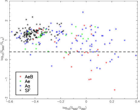
Figure 1: Radio sources with a 500-$\mu$m detection plotted on the diagnostic plot of López-Caniego et al. (2012). Colours indicate different emission-line classes. The dashed line indicates the threshold in FIR/radio radio used by López-Caniego et al. (2012); below this line, synchrotron emission might be bright enough to affect the SPIRE bands.

While the large number of non-detections in the GMRT survey means that we cannot carry out a detailed analysis, we note first of all that the mean spectral index of detected sources is close enough to our previously adopted value of 0.8 that our $K$-correction in the radio will not be badly in error, and secondly that the mean spectral index of the AeB objects is very much flatter than any of the other emission-line classes, although there is still clearly a population of steep-spectrum AeBs. Given that the detected objects are likely to be biased, if at all, towards the steep-spectrum end of the intrinsic distribution, it seems likely that the AeB objects contain a significant number of flat-spectrum quasars.

We investigated this issue further by considering the diagnostic methods used by López-Caniego et al. (2012) in searching for blazars. They relied on detections at 500 $\mu$m, and, as noted above, only a small fraction of our sources have $2\sigma$ detections at that band. We plotted the sources that do on the diagnostic radio/FIR colour-colour diagram used by López-Caniego et al. (2012), which is intended to search for non-thermal contamination in the SPIRE bands; the result is shown in Fig. 1. We see that of the 24 AeB objects with 500-$\mu$m detections, about half lie in the region occupied by the López-Caniego blazar candidates in which synchrotron emission might affect the SPIRE bands, a much higher fraction than for any other emission-line class. While red 500/350-$\mu$m colours may just be an indication of low dust temperatures, and the AeB sources have higher redshifts than the comparison objects, this is a further sign that the AeBs cannot safely be merged with the Ae objects in what follows.

3.2 Herschel and radio luminosity

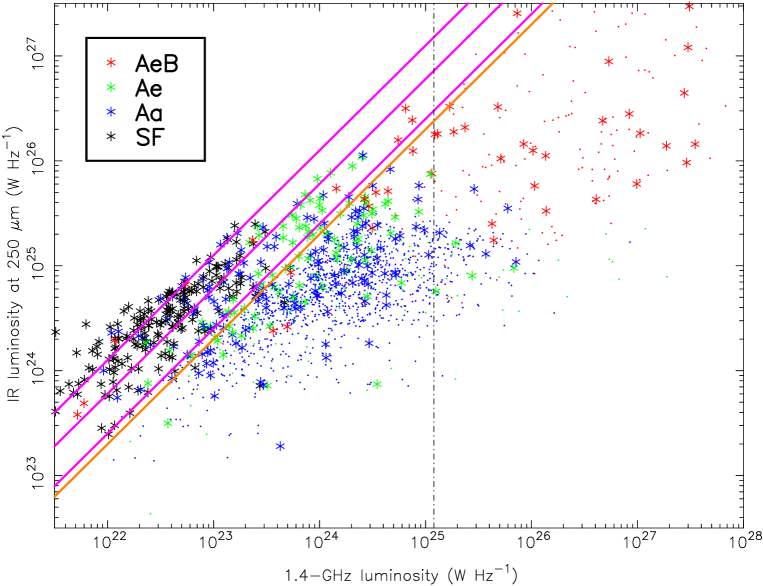
Figure 2: 250-$\mu$m luminosity against radio luminosity for all the objects in the sample. Stars indicate Herschel detections at $2\sigma$ or better as defined in the text, points show $2\sigma$ upper limits in IR luminosity derived from the confusion limit. Colours correspond to emission-line classes as follows: Aa, blue; Ae, green; AeB, red; SF, black. The solid magenta lines indicate the expected radio-FIR correlation for star-forming objects, $q_{\rm 250}=1.78$, and the approximate scatter about this relation, $1.4<q_{250}<2.1$ (from Jarvis et al., 2010). The solid orange line shows our adopted ‘SF cut’ at $q_{250}=1.3$, and the dot-dashed vertical line shows the nominal FRI/FRII break luminosity.

Fig. 2 shows the IR luminosity, $L_{250}$, against the radio luminosity for all the objects in the sample. This plot shows several important features of the sample. First, we note that the vast majority of the broad-line objects (in red) lie at the very high-luminosity end of the plot, presumably due to their high redshifts. As we noted above that some of these objects may well have FIR fluxes contaminated by non-thermal emission, and as their high redshift makes it difficult to compare them with radio galaxies in any case, we exclude them from further analysis.

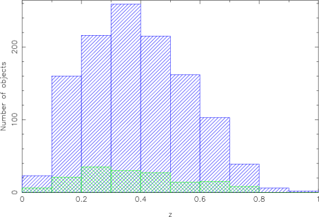
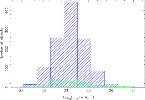
Figure 3: The distribution of (left) redshift and (right) radio luminosity in the Aa (blue) and Ae (green) objects after the SF cut. The redshift and luminosity distributions of the samples are very similar.

Fig. 2 also shows the expected linear radio-FIR correlation for star-forming objects (magenta lines), together with the dispersion seen in that relationship, based on the parameter $q_{250}$, which is defined as $\log_{10}(L_{250}/L_{1.4})$ (Jarvis et al., 2010). We see that objects classed as SF on the basis of their emission-line properties or their radio/H$\alpha$ relation (black points) almost all lie in this region of the plot and close to the best-fitting line; there is some positive deviation above the line at low luminosities/redshifts, but this was also seen by Jarvis et al.. However, at higher luminosities, a number of objects of other emission-line classes also fall in the star-forming region, meaning that their radio emission is not bright enough to definitively classify them as radio galaxies. Conservatively, every object that lies in the star-forming region of this plot should be excluded from a discussion of the FIR properties of radio galaxies; following V12, we adopt a cut at $q_{250}\geq 1.3$. The numbers of sources remaining, if these objects are excluded, are given in Table 1. The vast majority of the SF objects are removed by the cut (hereafter the ‘SF cut’), and although some of the 8 remaining sources may be radio galaxies which have erroneously been classified as SF, we conservatively exclude them from subsequent analysis (given the small numbers involved, including them as though they were Ae objects would have little effect on our results).

Considering only the remaining objects, which we expect to be radio-loud AGN, we see that these span a very large range in radio luminosity, from $10^{22}$ to $10^{27}$ W Hz^-1 if we ignore the broad-line objects. The vast majority of these lie below the nominal FRI-FRII luminosity divide (Fanaroff & Riley, 1974) of $1.2\times 10^{25}$ W Hz^-1 (plotted on Fig. 2 for reference) and so would normally be classed as low-luminosity radio galaxies, though we emphasise that the FRI/FRII division is a morphological one and we have made no attempt to classify these objects morphologically. In terms of our observational emission-line classifications, we see that Aa objects dominate numerically by a large factor, but that there are Ae objects at all powers. Assuming that Aas trace LERGs and Aes HERGs, this is consistent both with what is seen in brighter radio-selected samples at low redshift (see, e.g., Hardcastle et al., 2009) and with the work of Best & Heckman (2012) over a comparable luminosity range. The Aa and Ae objects left after the SF cut has been made have redshift and radio luminosity distributions that are indistinguishable on a KS test (Fig. 3), but this is not surprising, since the differences in the slope of the luminosity function for the two populations, leading to the dominance of HERGs at high luminosities, start to become significant only at $L_{1.4}>10^{25}$ W Hz^-1 (Best & Heckman, 2012), where we have relatively few sources.

3.3 LERG/HERG comparisons and stacking

Some differences between the FIR properties of the Aa and Ae objects after the SF cut are immediately obvious on inspection of the data. For example, 53/156 (34 per cent) of the Ae objects are detected at the $2\sigma$ level or better at 250 $\mu$m, while only 93/1186 (8 per cent) of the Aa objects are detected at this level.

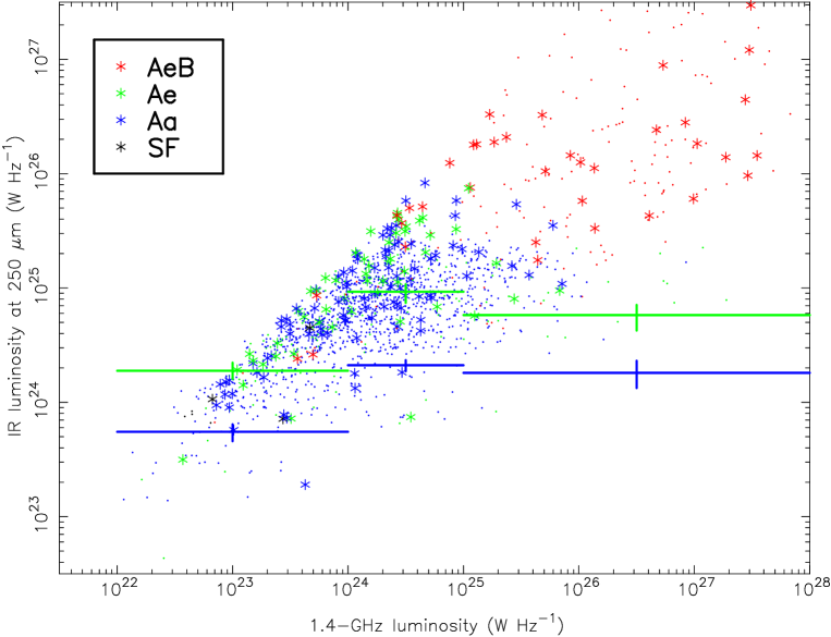
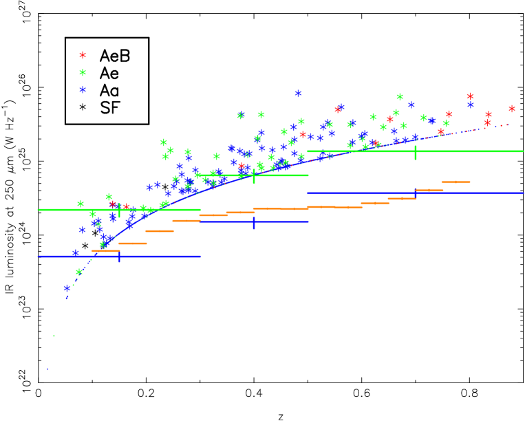
Figure 4: Comparisons between the IR luminosities of the Aa and Ae objects, after excluding objects near the star-formation line, as a function of (top) radio luminosity and (bottom) redshift. Symbols and colours as for Fig. 2. The large crosses indicate the results of stacking the IR luminosities of all Ae (green) and Aa (blue) objects in the corresponding radio luminosity or redshift range. Other types of object are plotted but not stacked. The orange bins indicate stacking of comparison galaxies, as described in the text.

Overall, both individual sub-samples still being considered (i.e. Aa and Ae after SF cut) are significantly detected with respect to the background at all three Herschel-SPIRE bands. We follow H10 in testing this with a KS test on the distribution of flux densities compared to random flux densities from the field; the highest null hypothesis probability is $6.6\times 10^{-8}$ for the Aa sources at 500 $\mu$m, corresponding to a minimum significance of $5.5\sigma$ for both classes and all SPIRE bands, and the significance is much higher at 250 $\mu$m. For the two PACS bands, the Aa sub-sample is detected at around 98 per cent confidence (i.e. a marginal detection, $2.3\sigma$) but the Ae objects are significantly detected with a null hypothesis probability around $2\times 10^{-7}$ ($5.2\sigma$).

We are therefore able to adopt the approach of H10 and divide our sources into luminosity and redshift bins for a stacking analysis. Since we have relatively few Ae sources, we use only three bins in both, ensuring that the highest-luminosity bin includes all sources above the nominal FRI/II luminosity boundary at $L_{1.4}=1.2\times 10^{25}$ W Hz^-1, which, as noted above, can roughly be taken to separate ‘low-power’ and ‘high-lower’ radio galaxies. We then used KS tests to see whether these subsamples were detected (distinguished from the background flux density distribution) at each of the five H-ATLAS wavelengths. The results are shown in Tables 3 and 4.

Table 3: Mean bin flux densities and K-S probabilities that the Herschel fluxes of objects in redshift bins (after the SF cut) are drawn from the background distribution, as a function of emission-line class and wavelength. Low probabilities (below 1 per cent) imply significant differences between the bin being considered and the distribution of flux densities measured from randomly selected positions in the sky, as described in the text. Note that the bins do not include quite all the objects in the sample.

Class	$z$ range	Objects	Mean bin flux density (mJy)					K-S probability (%)
		in bin	SPIRE bands			PACS bands		SPIRE bands			PACS bands
			250 $\mu$m	350 $\mu$m	500 $\mu$m	100 $\mu$m	160 $\mu$m	250 $\mu$m	350 $\mu$m	500 $\mu$m	100 $\mu$m	160 $\mu$m
Aa	0.00 – 0.30	399	$5.5\pm 0.3$	$1.0\pm 0.4$	$2.5\pm 0.4$	$2.7\pm 1.5$	$8.7\pm 1.9$	$<10^{-3}$	$<10^{-3}$	0.3	2.2	3.6
	0.30 – 0.50	475	$4.7\pm 0.3$	$0.7\pm 0.3$	$2.1\pm 0.4$	$3.1\pm 1.4$	$7.0\pm 1.7$	$<10^{-3}$	0.004	0.09	46.1	9.9
	0.50 – 0.90	310	$5.3\pm 0.4$	$1.4\pm 0.4$	$2.6\pm 0.5$	$0.2\pm 1.7$	$5.9\pm 2.1$	$<10^{-3}$	$<10^{-3}$	0.01	41.1	35.4
Ae	0.00 – 0.30	62	$27.9\pm 0.9$	$10.2\pm 0.9$	$6.4\pm 1.1$	$68.2\pm 3.8$	$50.3\pm 4.6$	$<10^{-3}$	$<10^{-3}$	0.05	$<10^{-3}$	0.06
	0.30 – 0.50	57	$22.8\pm 0.8$	$8.1\pm 0.9$	$3.8\pm 1.1$	$25.6\pm 3.8$	$30.7\pm 4.7$	$<10^{-3}$	0.005	2.1	0.3	1.5
	0.50 – 0.90	37	$20.4\pm 1.0$	$9.8\pm 1.2$	$7.6\pm 1.4$	$23.5\pm 5.0$	$14.2\pm 6.1$	$<10^{-3}$	0.002	0.10	11.9	20.8

Table 4: Mean bin flux densities and K-S probabilities that the Herschel fluxes of objects in luminosity bins (after the SF cut) are drawn from the background distribution, as a function of wavelength. Notes as for Table 3.

Class	Range in	Objects	Mean bin flux density (mJy)					K-S probability (%)
	$L_{1.4}$	in bin	SPIRE bands			PACS bands		SPIRE bands			PACS bands
			250 $\mu$m	350 $\mu$m	500 $\mu$m	100 $\mu$m	160 $\mu$m	250 $\mu$m	350 $\mu$m	500 $\mu$m	100 $\mu$m	160 $\mu$m
Aa	22.0 – 24.0	457	$4.7\pm 0.3$	$0.5\pm 0.3$	$1.9\pm 0.4$	$3.2\pm 1.4$	$6.9\pm 1.8$	$<10^{-3}$	0.002	0.2	2.1	14.5
	24.0 – 25.0	589	$5.7\pm 0.3$	$1.5\pm 0.3$	$2.6\pm 0.3$	$2.4\pm 1.2$	$7.5\pm 1.5$	$<10^{-3}$	$<10^{-3}$	$<10^{-3}$	49.6	8.1
	25.0 – 28.0	140	$3.6\pm 0.5$	$0.7\pm 0.6$	$2.8\pm 0.7$	$-1.7\pm 2.5$	$7.4\pm 3.1$	0.006	0.4	1.8	34.0	19.8
Ae	22.0 – 24.0	71	$19.0\pm 0.8$	$6.3\pm 0.9$	$3.7\pm 1.0$	$27.2\pm 3.4$	$30.7\pm 4.2$	$<10^{-3}$	$<10^{-3}$	1.7	0.006	2.0
	24.0 – 25.0	57	$35.3\pm 0.8$	$14.2\pm 0.9$	$8.0\pm 1.1$	$69.2\pm 4.0$	$52.5\pm 4.8$	$<10^{-3}$	$<10^{-3}$	0.01	0.002	0.09
	25.0 – 28.0	28	$15.2\pm 1.2$	$7.2\pm 1.3$	$6.4\pm 1.6$	$24.3\pm 5.6$	$7.8\pm 7.0$	$<10^{-3}$	0.004	0.4	4.0	94.5

As found by H10, the detection of all our subsamples is best at 250 $\mu$m, although with this larger sample most bins are significantly detected at 350 $\mu$m as well (see Tables 3 and 4). 500-$\mu$m detections are less robust, and only the low-redshift Ae subsamples are significantly detected in the PACS bands. We therefore rely on the 250 $\mu$m flux densities for our first estimate of luminosities. With the division of the samples into the two emission-line classes, we can see that the mean 250-$\mu$m flux density for the Ae objects is much higher than for the Aa objects in every bin.

Our stacking analysis follows the method of H10; we determine the luminosity for each source from the background-subtracted flux density, even if negative, on the grounds that this is the maximum-likelihood estimator of the true luminosity, and take the weighted mean within a bin to estimate stacked bin luminosities. Unlike H10, we determine errors on the bins by bootstrapping, having verified that this method gives very similar results to the much more time-consuming and complex method used in the earlier paper. As Fig. 4 shows, we find a clear and significant difference between the FIR luminosities of the Ae and Aa objects in every bin in either radio luminosity and redshift.

3.4 Comparison with normal galaxies

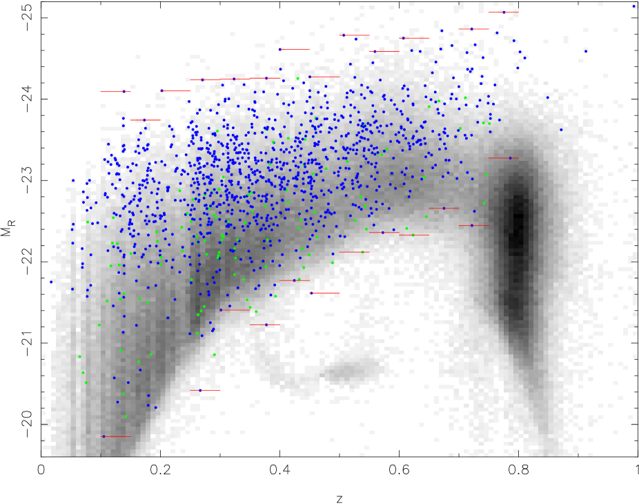
Figure 5: The $M_{R}$-redshift distribution ($K$-corrected as described in the text) of sample objects in the Aa (blue) and Ae (green) classes, after the ‘SF cut’, plotted on top of the same information for the comparison galaxies discussed in the text (greyscale shows a density plot with square-root transfer function). Red lines show the range of absolute magnitudes of the radio-selected sample, used to generate the comparison galaxy sample discussed in the text. The peak in redshift around $z\approx 0.8$ is probably an artefact of the photometric redshifting, but does not affect our comparison sample.

As a result of our procedure for generating our radio galaxy catalogue in H10, we automatically had a comparison galaxy population. There is no equivalent in the present work, in the sense that there is no galaxy population selected in the same way as the radio-loud objects. Spectroscopic redshifts for the GAMA sample run out at around $z\sim 0.6$ because of the magnitude limit used by GAMA (Driver et al., 2011) while our spectroscopic sample extends to fainter galaxies and higher redshifts. However, a rough comparison with radio-quiet galaxies is useful to put our results in context. We therefore constructed a comparison galaxy sample as follows:

1. We based the sample on the galaxy catalogue over the Phase 1 fields provided as part of the H-ATLAS data release, constructed in the manner described by Smith et al. (2011), and selected galaxies that had either a spectroscopic redshift (from GAMA or SDSS) or a photometric redshift with nominal error $<0.1$, had measured SDSS $r$ and $i$ magnitudes, and were not point-like in $r$ or $i$.

2. From this sample we took all objects which lay on the observed H-ATLAS fields and measured their background-subtracted 250-$\mu$m flux densities as for the radio galaxies (giving 318,244 objects in total, the vast majority with only photometric redshifts). We excluded at this point all objects that formed part of the radio-galaxy sample.

3. We $K$-corrected the $r$-band absolute magnitudes of the radio galaxies and the comparison sample to $z=0$ using kcorrect v. 4.2 (Blanton & Roweis, 2007).

4. Comparing the range of $r$-band absolute magnitude in the radio-galaxy sample with that in the comparison galaxies (Fig. 5) we saw that the radio-selected objects tend to be bright galaxies at all redshifts. At lower $z$ there is a tendency for the Ae galaxies to be fainter than the Aa (as seen by, for example, Tasse et al. 2008 and Best & Heckman 2012; note that our sample is not complete, which reduces the extent to which we can draw conclusions from this observation), but they occupy similarly bright galaxies at high $z$ (Fig. 6).

5. Clearly for even a rough comparison we should compare the radio galaxies with optical objects of comparable magnitudes. In each of 14 bins of width $\Delta z=0.05$ between $z=0.1$ and $z=0.8$, we selected only the comparison galaxies that lay in the absolute $r$ magnitude range spanned by the Aa and Ae objects (post-SF cut) in that redshift range.

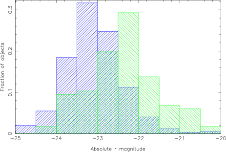
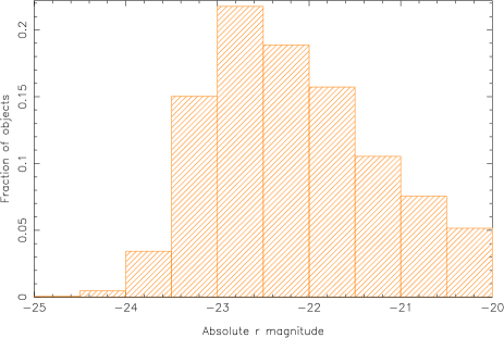
Figure 6: Histogram of (left) the absolute $r$ magnitudes of Aa (blue) and Ae (green) galaxies in the sample, after application of the SF cut, and (right) the absolute magnitudes of the comparison objects after the magnitude range selection. Aa objects are generally more massive galaxies than Aes, but the distributions have substantial overlap; the distribution of comparison galaxy absolute magnitudes has an intermediate peak.

We then stacked the Herschel FIR luminosities of the galaxies in those 14 bins, deriving them from the 250-$\mu$m flux densities on the assumption $T=20$ K, $\beta=1.8$ in the same way as for the radio galaxies. These stacks are plotted as a function of $z$ on Fig. 4. We emphasise that this is intentionally a crude comparison: for example, we could also have performed a colour selection on the comparison galaxies, but this would have involved an investigation of the optical colours of the Aa and Ae objects, accounting for possible AGN contamination, which we wish to defer to a later paper (Ching et al., in prep.); similarly, we are not attempting to separate spirals and ellipticals in the comparison sample, and we have made no attempt to match the actual distributions of magnitudes (and thus stellar masses) of the comparison galaxies within the absolute magnitude ranges used (Fig. 6). Our optical selection, which is required to allow matching to the radio galaxies, also potentially biases us against the most strongly star-forming radio-quiet galaxies, which will tend to be more dust-obscured. However, the result of the comparison is clear. The luminosities for the comparison galaxies tend to lie in between those for the Aa and the Ae radio-loud objects; thus, in the redshift range where we have data, Ae galaxies are on average more luminous in the FIR than the average galaxy of comparable optical magnitude at a given redshift, and Aa galaxies are on average less luminous, at least in the low-redshift bins where a comparison is possible. We note that the comparison sample, though differently selected, is behaving in a very similar manner to that of H10 in terms of its FIR luminosity as a function of redshift; but now that we have a larger sample and can separate radio galaxies by emission-line class, we are able to see differences between the radio-loud and radio-quiet populations.

3.5 Individual dust temperatures and masses

Our large sample and the availability of the PACS data allow us to investigate the temperatures and isothermal dust masses (Section 2.4) of radio-selected objects for the first time.

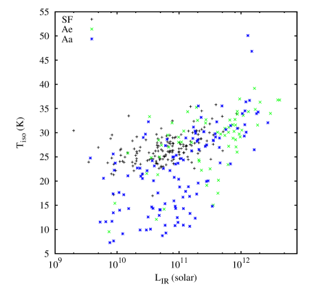
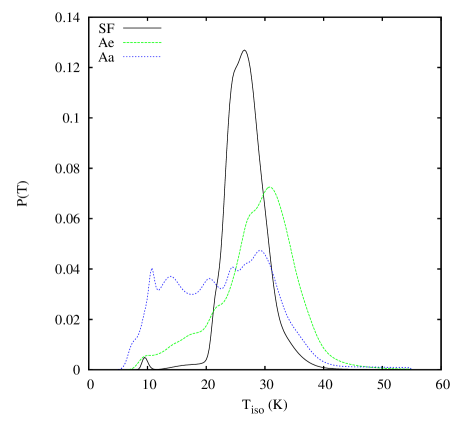
Figure 7: Left: a temperature-luminosity plot for the SF, Aa and Ae sources with individually determined temperatures. Right: stacked, normalized posterior distribution functions (PDFs) for temperature fits to the SF, Ae and Aa emission-line classes.

We began by fitting single-temperature modified black-body models to all the sources for which this was possible. We selected all objects which had a $2\sigma$ detection, as defined above, in at least two Herschel bands, in order to ensure that there was at least in principle sufficient signal-to-noise to constrain parameters, and then used standard Levenberg-Marquardt $\chi^{2}$ minimization to find the best-fitting values of temperature and normalization for the modified blackbody model to the flux densities measured at all five H-ATLAS bands.

One decision that has to be taken here concerns the emissivity parameter $\beta$. Earlier work, including H10 and Dunne et al. (2011), takes this to be 1.5, but work on local galaxies (e.g. Davies et al., 2012) has obtained good fits (using much better data than available to us) with $\beta=2$. Fitting for $\beta$ across the whole sample (marginalizing over temperature and normalization for each object) we find that the best fits are found with $\beta=1.8$ (the validity of this approach will be discussed by Smith et al., in prep). We fixed $\beta$ to this value and then fitted for temperature and normalization, determining errors by mapping the $\Delta\chi^{2}=2.3$ error ellipse (corresponding to $1\sigma$ for two parameters of interest). For these final fits, only individual fits with an acceptable $\chi^{2}$ value (defined as a reduced $\chi^{2}<2$) and a well-constrained temperature ($\Delta T/T<2$) are considered in what follows. This process gives us 385 measured temperatures and normalizations, including 128 Aa objects (10 per cent of the total), 70 Aes (35 per cent) and 170 SF objects (88 per cent); the ‘SF cut’ was not applied to the parent sample. Integrated FIR luminosity ($L_{\rm IR}$, integrated between 8 and 1000 microns) and isothermal dust masses were then calculated from the fitted temperature and normalization.

Clearly the quantities we measure in this way are expected to be biased towards the brightest and hottest objects, but it is still instructive to see how they relate to our emission-line classifications. Fig. 7 shows the temperature-luminosity and temperature-dust mass plots for these objects broken down by emission-line class. We exclude the broad-line objects, because of concerns noted above about contamination of the FIR bands by non-thermal emission. We see what appears to be a bimodal distribution of temperatures, with one set of objects, here seen to be mostly Aas, having temperatures in the range $10<T<20$ K, while the other, comprising most of the SF and Ae objects together with a significant minority of Aas, has $25<T<40$ K. The typical error bar on fitted temperature (not plotted for clarity) is of order 10 per cent. These temperatures generally seem realistic: the isothermal dust temperatures measured by Dunne et al. (2011) span the range 10–50 K, and, unsurprisingly, our temperatures also lie in this range, while temperatures measured for early-type galaxies in the Herschel Reference Survey (Smith et al., 2012b) are $\sim 24$ K, which is comparable to what we see for the Ae sample. What is more surprising is the cold temperatures found for a number of the Aa objects. Integrated temperatures of the order of 10 K are perhaps just plausible for dust in thermal equilibrium with the old stellar population of elliptical galaxies, if the distribution of dust is chosen carefully; Goudfrooij & de Jong (1995) show that temperatures of tens of K are expected for dust in the centres of elliptical galaxies, but the effective temperature should be an emission-weighted average over the dust distribution throughout the galaxy, and the energy density in photons falls off very rapidly with distance from the centre of the galaxy, so the integrated temperature depends on dust distribution, but could be substantially lower than the peak value. However, the lowest temperatures found by the fits would imply dust masses of up to $10^{10}M_{\odot}$, which is probably not realistic. Inspection of the images for the sources with very low temperatures suggests that several of them are the result of flux confusion: given our $2\sigma$ flux cuts, up to 30 of the Aa sources that we have fitted could be spurious detections, and while we do not expect the numbers to be this high in practice, confusion seems likely to account for a number of the sources with the lowest fitted temperatures and highest dust masses. In addition, synchrotron contamination of the SPIRE bands, which is observed in nearby LERGs like M87 (Baes et al., 2010) could be affecting a few Aas – several fall below the dividing line in the plot of Fig. 1, although not all of these will have the flat integrated radio spectrum required for non-thermal emission to appear at 500 $\mu$m.

Another way of investigating the temperature differences between the samples, which does not put so much weight on individual objects, is to consider the stacked posterior probability distribution over $T$, marginalizing over normalization, for the fitted objects, and this is shown in the right-hand panel of Fig. 7. Here a prior of $5<T<55$ K is used. We see that this plot reproduces the broad trends seen in the left-hand panel: the SF objects have a fairly well-defined peak in temperature at around 26 K, the Aes have a broader peak at around 30 K, and the Aas span a range between around 10 and 30 K. Even taking into account possible contamination by confused sources and/or synchrotron emission in a few cases, it does not seem likely that the Aa and Ae sources have the same intrinsic temperature distribution. In addition, it is hard to see how this difference in the PDFs could be explained by, for example, different $\beta$ values for different populations.

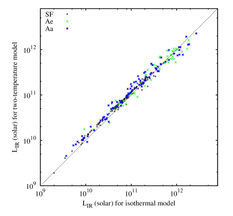
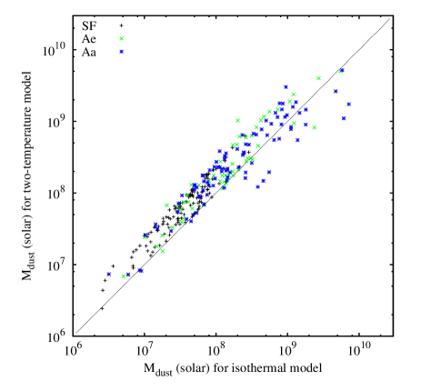
Figure 8: The relationships between (left) the integrated IR luminosity and (right) the dust mass for objects with fits of both a single-temperature and a two-temperature model.

It is natural to interpret the wide range of temperatures in the temperature-luminosity plots in terms of two populations of dust: (1), a cold dust component which is always present, which is essentially in thermal equilibrium with the old stellar population ($T\sim 15$ K might be reasonable for this as an average over the dust properties of an elliptical galaxy, as noted above) and whose mass scales with the total galaxy mass, perhaps with some redshift dependence; and (2), a warmer dust component with $T\sim 30$ K which traces current star formation and whose mass and luminosity are primarily an indicator of the star-formation rate (cf. Dunne et al., 2011; Smith et al., 2012a). In fact, such a two-temperature model might help to explain the lack of objects with $T\sim 20$ K in Fig. 7: although there should be objects where the two components contribute roughly equally to the Herschel SED, these would tend to be poorly fitted with a single-temperature model and would be rejected by our fitting procedure.

The type of broad-band fitting to the FIR through ultraviolet SEDs carried out by Smith et al. (2012a) is beyond the scope of this paper, but we investigated a two-temperature model by fitting the same dataset for the normalizations of two modified-blackbody models with $\beta=1.8$ and fixed temperatures of 15 K and 30 K (normalizations here are explicitly constrained to be positive to avoid trading off negative flux in one component against positive flux in another). These models in general fit less well and therefore give fewer sources with acceptable fits, presumably because there are objects with well-determined temperatures for the warm component that are significantly different from 30 K, but we do note that they provide good fits to a population of objects that are rejected by the $\chi^{2}$ criterion for the single-temperature fits and that generally have non-zero contributions to the dust luminosity from both hot and cold components. Moreover, and importantly for what follows, we find a good correlation between the total luminosities for objects where these can be obtained using both methods (Fig. 8), while the estimated dust masses show some systematic differences. This suggests that, at least for this sample, the total IR luminosity can be used without worrying too much about more complex models, while the dust mass must be interpreted with a little more care. If we interpret the mass of warm dust (or, equivalently for this model, its luminosity) in these fits as tracing star-formation rate, then, using the results of (Smith et al., 2012a), the typical SF object in our sample has a star-formation rate of $\sim 10M_{\odot}$ yr^-1, while the most luminous Ae objects might have star-formation rates more than ten times higher. More detailed methods for estimating star-formation rates are discussed in the following subection.

Finally, we note that the weighted mean of the best-fitting single temperatures of the Aas and Aes, for $\beta=1.8$, is 20.3 K. This justifies the assumptions we used for $K$-corrections in the luminosity stacking of Section 3.3.

3.6 $L_{250}$ as a star-formation rate indicator; comparing emission-line classes

As we noted in the previous subsection, contributions to $L_{250}$ are made both by cold dust (driven by the old stellar population) and warm dust (driven by star formation). It follows that neither $L_{250}$ nor the integrated $L_{\rm IR}$ are reliable indicators of star formation rates (SFR) in general. However, they should both be usable to estimate SFR for an object whose FIR emission is dominated by emission from warm dust: these will be the objects whose best-fitting temperatures are $\sim 25$ K or more. For objects with a contribution from cold dust, the SFR estimated from $L_{\rm 250}$ or $L_{\rm IR}$ will be an upper limit.

To use the quantity that we have used for stacking, $L_{\rm 250}$, in this way we need to calibrate the relationship between it and SFR. We choose to do this by considering the objects classed optically as ‘SF’, as, where temperature information is available, all of these have FIR temperatures consistent with being dominated by star formation (Section 3.5). For SF objects with SDSS spectra estimated star formation rates, derived using the methods of Brinchmann et al. (2004) (i.e. by model-fitting to the optical emission lines and stellar continuum), are available in the MPA-JHU database. Cross-matching our SF objects against this database gives a sample of 158 objects with both SFR and $L_{\rm 250}$ estimates; we use the median likelihood estimates given in the MPA-JHU database, as being the most robust, and take half the difference between the 16th and 84th percentiles as an estimate of the error on the SFR. As these objects are all at low redshifts ($z<0.24$, and median $z=0.08$) we need not be concerned about the $K$-correction used to derive $L_{\rm 250}$. When we plot $L_{\rm 250}$ against SFR derived in this way, we see a good correlation (Fig. 9) with a slope that is, by eye, close to unity. A Markov-Chain Monte Carlo regression, taking the errors on both SFR and $L_{\rm 250}$ into account and incorporating an intrinsic dispersion in the manner described by Hardcastle et al. (2009), gives Bayesian estimates of the slope and intercept of the correlation:

$$\log_{10}(L_{250}/{\rm W}\ {\rm Hz}^{-1})=23.64+0.96\log_{10}({\rm SFR}/M_{\odot}\ {\rm yr}^{-1})$$

Although a slope of unity is not ruled out, we will use this slightly non-linear relationship in what follows. We emphasise again that it is only valid for objects whose FIR emission is known to be dominated by warm dust heated by star formation.

As a sanity check on this approach, we can also estimate the relationship between SFR and integrated $L_{\rm IR}$ by using our temperature fits from Section 3.5. The vast majority (143) of SF objects with SFR estimates also have estimates of $T_{\rm IR}$ and thus $L_{\rm IR}$, and this quantity also correlates well with SFR (Fig. 9). Regression gives a linear relation

$$\log_{10}(L_{\rm IR}/L_{\odot})=9.90+1.00\log_{10}({\rm SFR}/M_{\odot}\ {\rm yr}^{-1})$$

whose normalization is only a factor 1.4 away from the standard relation given by Kennicutt (1998), derived for starbursts. Thus we can use our IR-derived SFR with reasonable confidence.

Applying the $L_{250}$/SFR relation to Fig. 4, we can see that the most luminous detected radio galaxies, at around $9\times 10^{25}$ W Hz^-1, should correspond to star-formation rates around 250 $M_{\odot}$ yr^-1, which does not seem unreasonable – these would be radio galaxies associated with starbursts – although it should be noted that there is a non-negligible uncertainty associated with the $L_{250}$ values of these luminous, high-$z$ sources because of the poorly known $K$-correction. Individual powerful, high-$z$ radio galaxies have been associated with star formation at levels even higher than this (Barthel et al., 2012; Seymour et al., 2012). The mean $L_{250}$ of the most radio-luminous Aes, with $L_{1.4}>10^{25}$ W Hz^-1, corresponds to $15M_{\odot}$ yr^-1, which is well above the SFRs expected for normal ellipticals in the local universe. The factor $\sim 4$ between the stacked $L_{250}$ values for Aes and Aas means that the mean star formation rate in the latter is at least a factor 4 below that in the Aes; ‘at least’ because the temperature measurements suggest that the emission from some, and perhaps most, Aas is dominated by cold dust.

Figure 9: The relationship between star-formation rate (SFR), determined for the SF class from the MPA-JHU emission-line database using the methods of Brinchmann et al. (2004), and the two types of FIR luminosity discussed in this paper, $L_{250}$ (left) and $L_{\rm IR}$ (right). The green lines show the results of a MCMC regression, as described in the text. Error bars are not plotted for clarity – the uncertainty on SFR can be $\pm 0.5$ dex.

3.7 Stacked dust temperatures, masses and SFR

Table 5: Results of temperature fitting, dust mass and star formation rate estimation in redshift bins.

Class	Range in	Objects	Best-fit $T$	Reduced	$\log_{10}(L_{250}/{\rm W}\ {\rm Hz}^{-1})$	$\log_{10}(M_{\rm iso}/M_{\odot})$	$\log_{10}({\rm SFR}/M_{\odot}\ {\rm yr}^{-1})$
	$z$	in bin	(K)	$\chi^{2}$
Aa	0.00 – 0.30	398	$17.0^{+0.9}_{-0.8}$	1.65	$23.9\pm 0.1$	$7.6\pm 0.1$	$0.2\pm 0.1$
	0.30 – 0.50	472	$17.4^{+0.6}_{-0.6}$	1.52	$24.3\pm 0.1$	$8.0\pm 0.1$	$0.7\pm 0.1$
	0.50 – 0.90	309	$27.8^{+2.1}_{-3.4}$	1.44	$24.6\pm 0.1$	$7.7\pm 0.1$	$1.0\pm 0.1$
Ae	0.00 – 0.30	62	$32.8^{+0.7}_{-0.8}$	2.11	$24.3\pm 0.1$	$7.3\pm 0.1$	$0.7\pm 0.1$
	0.30 – 0.50	55	$30.9^{+0.7}_{-0.8}$	1.45	$24.8\pm 0.1$	$7.8\pm 0.1$	$1.2\pm 0.1$
	0.50 – 0.90	36	$34.2^{+1.4}_{-1.5}$	1.99	$25.1\pm 0.1$	$8.0\pm 0.1$	$1.5\pm 0.1$

Table 6: Results of temperature fitting, dust mass and star formation rate estimation in luminosity bins.

Class	Range in	Objects	Best-fit $T$	Reduced	$\log_{10}(L_{250}/{\rm W}\ {\rm Hz}^{-1})$	$\log_{10}(M_{\rm iso}/M_{\odot})$	$\log_{10}({\rm SFR}/M_{\odot}\ {\rm yr}^{-1})$
	$\log_{10}(L_{1.4})$	in bin	(K)	$\chi^{2}$
Aa	22.0 – 24.0	456	$15.1^{+0.6}_{-0.5}$	1.50	$24.0\pm 0.1$	$7.9\pm 0.1$	$0.4\pm 0.1$
	24.0 – 25.0	589	$23.8^{+0.8}_{-0.7}$	1.65	$24.5\pm 0.1$	$7.7\pm 0.1$	$0.9\pm 0.1$
	25.0 – 28.0	140	$15.3^{+0.7}_{-0.6}$	1.48	$24.7\pm 0.1$	$8.6\pm 0.1$	$1.1\pm 0.1$
Ae	22.0 – 24.0	71	$26.3^{+0.6}_{-0.7}$	1.70	$24.3\pm 0.1$	$7.5\pm 0.1$	$0.7\pm 0.1$
	24.0 – 25.0	57	$30.9^{+0.5}_{-0.6}$	2.08	$25.0\pm 0.1$	$8.0\pm 0.1$	$1.5\pm 0.1$
	25.0 – 28.0	28	$27.0^{+1.7}_{-1.8}$	1.59	$24.9\pm 0.2$	$8.0\pm 0.2$	$1.3\pm 0.2$

As noted above, direct estimation of dust temperatures can only be carried out for the brightest (and possibly hottest) objects, and so might give misleading results if used in the interpretation of our stacking analysis of the whole sample. As an alternative, we can estimate mean temperatures for objects in the sample as follows. We bin our objects in redshift or radio luminosity as in the previous two sections. For each redshift/luminosity bin, we determine the single dust temperature that gives the best $\chi^{2}$ fit to the observed flux densities of every galaxy in the bin, allowing each galaxy to have a free normalization (which may be negative) and taking a fixed $\beta=1.8$. Errors in this fitted temperature are estimated by finding the range that gives $\Delta\chi^{2}=1$. We can then use the best-fitting temperature and normalizations for all the sources to estimate the 250-$\mu$m luminosity of the bins, determining error bars by bootstrap as before. The results of this process are tabulated in Tables 5 and 6. The $\chi^{2}$ fitting gives acceptable, though not particularly good results, as we would expect since, from the analysis of Section 3.5, we know that there is a wide range of temperatures in each bin. Nevertheless, we can attempt to interpret the results.

Three points are of interest. Firstly, we note that the luminosities we estimate are broadly consistent, within the errors, with the luminosities estimated from the stacking analysis of Section 3.3; this gives us confidence that the luminosities from the earlier analysis are reasonable and that the assumption of a single temperature for the $K$-correction does not have a big effect on the inferred monochromatic luminosities. The luminosity difference between the Aa and Ae spectral classes clearly persists in this analysis. Secondly, we see that the temperatures are systematically different for the two emission-line classes: Aes have systematically higher dust temperatures. Thirdly, we can compute isothermal dust masses from eq. 1 using the best-fitting temperature and mean luminosity – these are of course a complicated weighted mean of the dust masses of all the objects in the bin, but still gives us some information on the properties of the galaxies. These mean isothermal dust masses are tabulated for each bin in Tables 5 and 6. No very strong difference between the dust masses for the emission-line classes is seen in these mean masses. It therefore seems plausible that the clear observed difference in monochromatic FIR luminosity at 250 $\mu$m between the populations is driven by a difference in dust temperature rather than by dust mass.

Finally, we can attempt to convert the $L_{\rm 250}$ values from this fitting into star formation rates, using the results of Section 3.6. As already noted, this gives us upper limits if we have reason to suppose that some of the FIR emission comes from cold dust unrelated to star formation. The results of this conversion, given in the final column of Tables 5 and 6, must be treated with caution, therefore. Since the mean fitted temperatures of the Aes are $>30$ K, their SFR estimates may be a reasonable estimate of the true mean SFR in these systems; the same is not true of the Aas, and so, again, the safest interpretation is to say that the mean SFR in the Aes is of order a few tens of solar masses per year, and is at least $\sim 0.5$ dex higher than that in the Aas.

3.8 Radio source sizes

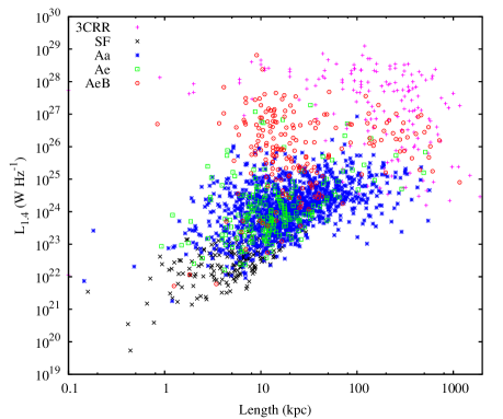
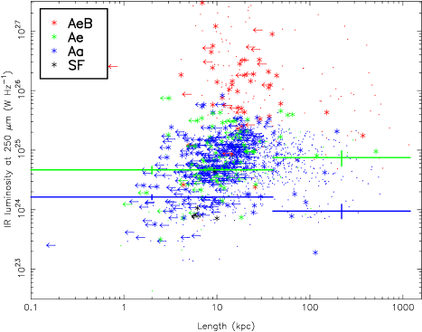
Figure 10: The physical sizes of radio sources in our sample and their relationship to radio and FIR luminosity. Left: the power/linear-size plot for the sample, broken down by emission-line class, and without the SF cut. Colours are as in Fig. 2; for comparison, 3CRR sources are plotted in magenta. Right: the FIR luminosity/linear size plot, with stacking in bins at $<40$ and $>40$ kpc, after the SF cut. Colours and symbols as in Fig. 2; upper limits in length are denoted by arrows.

V12 noted a strong relationship between the FIR luminosity or temperature of the objects they studied and the radio source size, in the sense that larger objects had systematically lower $L_{250}$ or $T$. They also showed that this discrepancy was largely driven by the most massive objects in their sample.

It is clearly interesting to ask how this result relates to the observed differences between emission-line classes. One of us (JSV) therefore determined the largest angular size of every object in the present sample, taking the sizes used by V12 for objects in common between the two samples and otherwise making measurements directly from the FIRST images. Where objects were unresolved in FIRST, an upper limit was assigned, as described by V12. Scaling by the angular size distance, this gives the distribution of source physical sizes for the current sample.

An important caveat in this analysis is that the current sample is not complete. This is illustrated by the left panel of Fig. 10, which shows the power/linear-size plot (the ‘$PD$ diagram’) for the current sample together with the equivalent plot for the complete and well-studied 3CRR sample. For clarity, upper limits are not marked on this plot, but it should be noted that all sources with a physical size $\geq 40$ kpc are actually resolved. We see that all emission-line classes are heavily biased towards smaller physical sizes with respect to 3CRR: of course, this is not a completely fair comparison, since the 3CRR objects are the most luminous objects in the radio sky at any given redshift, and we might expect lower-luminosity sources to be systematically smaller than the most luminous ones. However, there are more subtle signs of bias, such as the fact that there are more large AeB sources than there are Aes: this arises principally because a broad-line object is more likely to have a bright radio core and so to be identified with a galaxy or quasar in our original selection (though there is an additional effect due to the different redshift distribution of AeBs and Aes). The Aa sources, which should have the full range of angles to the line of sight, have a length distribution intermediate between the Aes and AeBs, as expected. This bias towards compact sources, or sources with compact cores, is particularly problematic for our sample because of the selection from FIRST radio images, which resolve out large-scale emission: the sample of V12 will be closer to being complete.

Having said this, it is still possible to investigate the FIR properties as a function of length. To do this we apply the SF cut and then stack the FIR luminosities as in Section 3.3, binning by length: we use only two length bins and the division is set at 40 kpc to ensure that all upper limits are in the correct bin. The results are shown in Fig. 10 (right panel). We see first of all that the Ae/Aa difference persists in this analysis: Ae sources have higher $L_{250}$ than Aas irrespective of length. Secondly, we see no evidence for any length dependence of the $L_{250}$ of the Ae population, although the error bars are large because the sample is small. Thirdly, we note a marginally significant difference between the $L_{250}$ values for the small and large Aa sources, in the sense noted by V12: the null hypothesis that these two are equal can be rejected at the 95 per cent confidence level. If, instead of stacking $L_{250}$, we fit temperatures to all the sources in each bin as described in Section 3.7, we find no significant difference in luminosities as a function of length for either emission-line class, but there are significant differences in best-fitting temperature ($29.4\pm 0.5$ vs $22\pm 2$ K for Ae; $21.8\pm 0.5$ vs $12.2\pm 0.4$ K for Aa), in both cases in the sense that the larger objects have lower best-fitting temperatures. This is again broadly consistent with the results of V12.

4 Discussion

The results of the previous section show very clearly that there is a difference between the average far-infrared properties of radio galaxies whose spectra show strong emission lines and those of radio galaxies that do not. How can we interpret this?

It is first of all important to consider the issue of possible AGN contamination, discussed in Section 1, in more detail. There are two possible sources for this: (1) emission from the warm dusty torus, which is expected to be seen predominantly in HERGs, and (2) synchrotron emission from the jets and lobes, which may appear in all objects. The first of these is particularly important, as torus-related emission in the FIR bands might give rise to a HERG/LERG difference, but we are confident that it is not a significant effect in our sample, for several reasons. Firstly, when the required mid-IR data are available, which is not the case for our sample at present, decompositions of the SEDs of radio-loud and radio-quiet AGN tend to show that observer-frame Herschel SPIRE bands are dominated by cool dust rather than by the torus component, even for powerful AGN with luminous tori (e.g Barthel et al., 2012; Del Moro et al., 2012). Secondly, we know, as pointed out by H10, that the mid-IR torus luminosities even for the most powerful HERGs in our sample, if they follow the correlation between radio power and mid-IR luminosity established by Hardcastle et al. (2009), should be about two orders of magnitude less than the total FIR luminosities estimated e.g. in Fig. 7, implying that even if the torus SEDs were strikingly different from those of known radio-loud AGN, it would still be energetically impossible for them to affect the observed FIR emission significantly. The second possible source of contamination, synchrotron emission, we believe to affect mostly the broad-line objects, as discussed in Section 3.1, together with at most a very few of the Aas; there is certainly no reason to expect that it would give rise to the observed Aa/Ae difference, since the radio fluxes and spectra of these two classes are very similar. We therefore consider it safe to discuss our observations in terms of a difference in the properties of cool dust in the two populations.

Our result cannot be significantly affected by contamination by pure star-forming objects whose radio emission is bright enough to cause them to be misidentified as radio galaxies. While our spectroscopic classification alone does not identify all objects whose radio emission is dominated by star formation (Fig. 2) the combination of optical spectroscopy and the ‘SF cut’ that we impose on the radio-FIR luminosity plane, where a clear star-forming sequence is visible, should remove all such objects. Moreover, the highest radio luminosities in our sample are well above even the $\sim 10^{25}$ W Hz^-1 expected from a starburst of a few thousand $M_{\odot}$ yr^-1, and we see a clear difference between the different emission-line classes in this luminosity range.

Along similar lines, we do not believe that the relationship between emission-line class and FIR emission can be a result of optical emission-line activity due to the star formation process itself. Our emission-line classification uses [Oiii], which, at least at high luminosities, is widely used as an AGN indicator, although it can be produced by hot, young stars. We do not have a direct estimate of the [Oiii] luminosities of our sample objects in the version of the GANDALF-derived database we use, but we have derived a rough indicator of luminosity from the measured equivalent widths and the $K$-corrected absolute magnitude in the SDSS $g$ band. Calibrating this indicator using the MPA-JHU emission-line measurements, for which both equivalent width and [Oiii] flux are tabulated, we see that almost all the Ae objects would be expected to have $L([\rm{O\hskip 0.56917pt\scriptscriptstyle{III}}])>10^{40}$ erg s^-1, and are thus in the range classified by e.g. Kauffmann et al. (2003) as ‘strong AGN’. Further work in this area will require measurements of the [Oiii] fluxes, and ideally those of other lines, for a large radio-galaxy sample, but we are confident that we are assessing genuine AGN activity in the vast majority of cases.

We can therefore move on to interpreting the relationship as being one between FIR properties of the host galaxy and the AGN-related emission-line properties of radio galaxies that we discussed in Section 1, with the Aa population corresponding to LERGs and the Ae population to HERGs. It then appears that HERGs, on average, have significantly higher $L_{250}$ than LERGs (Section 3.3); moreover, HERGs appear to have higher $L_{250}$ than normal galaxies of comparable absolute magnitude at all redshifts (Section 3.4). In a simple isothermal model, higher luminosity can arise either because of higher masses of dust or higher temperatures; what we see from the analysis of Sections 3.5 and 3.7 is that it is plausible that the dust masses of the different systems are similar, but that the mean isothermal temperatures of the HERGs are higher. In resolved local galaxies, it has been shown that low-temperature dust emission ($T\sim 15$ K) is driven by the old stellar population, while significantly hotter temperatures are seen from star-forming regions (e.g. Bendo et al., 2010; Boquien et al., 2011). By far the most obvious interpretation of our result is therefore that the star-formation rates are significantly higher in the HERG subsamples than in the LERGs, giving rise to a significant component of emission from hot dust which raises the isothermal temperature as seen in the analysis of Dunne et al. (2011). If so, this is strong confirmation, using a much larger sample, of the picture that emerges from the earlier work discussed in Section 1 (e.g. Baldi & Capetti, 2008; Herbert et al., 2010; Ramos Almeida et al., 2011b, 2012). By calibrating $L_{\rm 250}$ as a star formation indicator using SFRs derived from local radio-loud star-forming galaxies (Section 3.6) we have been able to quantify this, showing that the mean SFR in the most luminous/high-$z$ Aes is probably at the level of around $30M_{\odot}$ yr^-1, and is at least $\sim 0.5$ dex higher than that in the Aas at all redshifts and radio luminosities.

What does this tell us about the association between star formation and AGN activity in radio galaxies? The first point to note is that the association between a HERG classification and increased FIR luminosity (and therefore star-formation rate) is statistical only. It can be seen from Fig. 4 that there are individual LERGs with high FIR luminosities, while at the same radio luminosity we see HERGs with FIR luminosities 0.5-1 dex lower. Similarly, the temperature analysis of Section 3.5 shows that there are LERGs with best-fitting temperatures comparable (within the large errors) to those of the warm dust in known star-forming galaxies. Nothing appears to require HERGs to be associated with high star-formation rates or LERGs to be associated with completely quiescent galaxies, consistent with the conclusions of Tadhunter et al. (2011). This suggests that the mechanism of the association is not the simplest possible one, in which some single event, such as a merger, always triggers both HERG activity and star formation. If this were the case, we would not see individual LERGs with high star-formation rates (setting aside the possibility, which we regard as remote, that these sources are all misidentified HERGs).

Another piece of evidence supporting this picture comes from the lobe length analysis of Section 3.8. If HERGs were associated with AGN triggering following a merger, we might expect them to show a very strong relationship between FIR properties and lobe physical size, since star formation would be expected to peak on average at early times in the radio source’s lifetime. This was a possible interpretation of the results of V12, who showed that larger sources in general have lower FIR temperatures and luminosities. However, our analysis shows that this result is not driven by the HERG (Ae) population, and in fact for our sample is more obvious for the LERGs (which, however, have considerably better statistics).

We would therefore argue that we are not seeing a simple triggering relationship, but rather that the difference between HERGs and LERGs is that HERGs tend to inhabit environments in which star formation is favoured relative to the general galaxy population, while by contrast star formation is disfavoured in the environments of LERGs. The FIR differences as a function of source length would then be explained by some other process, such as jet-induced star formation when the bow shock of the source is within the host galaxy, which can in principle take place in both emission-line classes (although we note there is not yet any direct evidence for this process affecting emission seen in the FIR band). Such a model is consistent both with all the observations to date (e.g. Baldi & Capetti, 2008; Herbert et al., 2010; Best & Heckman, 2012; Janssen et al., 2012) and with the explanation of the HERG/LERG dichotomy in terms of accretion mode discussed in Section 1. It will be of great interest to see whether this result is confirmed by the larger samples that will be made available by the full H-ATLAS dataset, whether it can be extended to higher redshifts using deeper spectroscopic or photometric surveys, and whether the same results are obtained when the HERG/LERG classification is made using data at other wavebands (e.g. X-ray or mid-IR).

5 Summary and conclusions

The key results from the analysis and discussion above can be summarized as follows:

• We have used individual measurements and stacking analyses to determine the FIR properties (mean luminosities and temperatures) of a large sample of radio-selected sources with spectroscopic redshifts and HERG/LERG classifications from optical spectroscopy. Sources near the known FIR-radio correlation are excluded from our analysis; the vast majority of the objects we study should be bona fide radio galaxies.

• We find a clear difference between the FIR properties of the two populations in the sense that the rest-frame 250-$\mu$m luminosities are systematically higher in the HERGs than in the LERGs; the host galaxies of LERGs in fact occupy galaxies with lower FIR luminosities than normal galaxies matched in absolute magnitude, while HERGs tend to have higher FIR luminosities. This difference is apparent at all redshifts and all radio luminosities sampled by our targets.

• A comparison of the temperatures and dust masses of HERGs and LERGs, stacked in coarse bins, suggests that the dust masses are reasonably comparable for the two samples but that the temperatures in the HERGs are systematically higher. This provides strong evidence that the higher FIR luminosities we are seeing imply, on average, higher star formation rates (which are required to raise the mean temperature of the dust) rather than just higher dust masses. The low mean temperatures seen for LERGs are consistent with what would be expected for quiescent dust which is in thermal equilibrium with the photon field of the old stellar population of the host galaxy, although the fact that these objects are detected at all implies that large masses of dust are present.

• Quantifying the SFR by calibrating $L_{250}$ as a star-formation indicator in the ‘SF’ sources known to be dominated by hot dust, we find that the mean SFR in the radio-luminous Aes is $\sim 30M_{\odot}$ yr^-1, and is at least $\sim 0.5$ dex higher than that in the Aas at all luminosities and redshifts.

• Consistent with the results of V12, we find that both emission-line classes in our sample show some evidence for a dependence of FIR properties on radio source size.

• We argue that there is certainly not a simple triggering relation, and not even a one-to-one association, between enhanced star formation and a particular AGN type (a conclusion consistent with detailed studies of starburst radio galaxies such as that of Tadhunter et al., 2011). However, the statistical trend for HERGs to have higher star formation rates is consistent both with what is known from other wavebands (e.g. Best & Heckman, 2012; Janssen et al., 2012) and with the general class of models (Hardcastle et al., 2007) in which HERG activity takes place in lower-mass galaxies where the black hole is able to accrete significant quantities of cold gas.

As more H-ATLAS data and supporting optical imaging and spectroscopy become available we expect to extend this work to much larger samples, allowing more detailed binning and temperature analysis, to investigate different methods of carrying out the LERG/HERG classification, and to consider radio galaxies at higher redshifts in order to search for evidence of cosmological evolution of the star-formation properties of the radio-loud AGN population.

REFERENCES

- Adelman-McCarthy et al. (2008) Adelman-McCarthy J. K. et al., 2008, ApJS, 175, 297
- Archibald et al. (2001) Archibald E. N., Dunlop J. S., Hughes D. H., Rawlings S., Eales S. A., Ivison R. J., 2001, MNRAS, 323, 417
- Baes et al. (2010) Baes M. et al., 2010, A&A, 518, L53
- Baldi & Capetti (2008) Baldi R. D., Capetti A., 2008, A&A, 489, 989
- Baldwin et al. (1981) Baldwin J. A., Phillips M. M., Terlevich R., 1981, PASP, 93, 5
- Barthel et al. (2012) Barthel P., Haas M., Leipski C., Wilkes B., 2012, ApJ, 757, L26
- Becker et al. (1995) Becker R. H., White R. L., Helfand D. J., 1995, ApJ, 450, 559
- Bendo et al. (2010) Bendo G. J. et al., 2010, A&A, 518, L65
- Best & Heckman (2012) Best P. N., Heckman T. M., 2012, MNRAS, 421, 1569
- Best et al. (2006) Best P. N., Kaiser C. R., Heckman T. M., Kauffmann G., 2006, MNRAS, 368, L67
- Best et al. (2005) Best P. N., Kauffmann G., Heckman T. M., Brinchmann J., Charlot S., Ivezić Z., White S. D. M., 2005, MNRAS, 362, 25
- Blanton & Roweis (2007) Blanton M. R., Roweis S., 2007, AJ, 133, 734
- Boquien et al. (2011) Boquien M. et al., 2011, AJ, 142, 111
- Brinchmann et al. (2004) Brinchmann J., Charlot S., White S. D. M., Tremonti C., Kauffmann G., Heckman T., Brinkmann J., 2004, MNRAS, 351, 1151
- Chiaberge et al. (2002) Chiaberge M., Macchetto F. D., Sparks W. B., Capetti A., Allen M. G., Martel A. R., 2002, ApJ, 571, 247
- Condon et al. (1998) Condon J. J., Cotton W. D., Greisen E. W., Yin Q. F., Perley R. A., Taylor G. B., Broderick J. J., 1998, AJ, 115, 1693
- Croton et al. (2006) Croton D. et al., 2006, MNRAS, 365, 111
- Davies et al. (2012) Davies J. I. et al., 2012, MNRAS, 419, 3505
- Del Moro et al. (2012) Del Moro A. et al., 2012, ArXiv e-prints:1210.2521
- Di Matteo et al. (2005) Di Matteo T., Springel V., Hernquist L., 2005, Nature, 433, 604
- Dicken et al. (2009) Dicken D., Tadhunter C., Axon D., Morganti R., Inskip K. J., Holt J., González Delgado R., Groves B., 2009, ApJ, 694, 268
- Dicken et al. (2012) Dicken D. et al., 2012, ApJ, 745, 172
- Driver et al. (2011) Driver S. P. et al., 2011, MNRAS, 413, 971
- Driver et al. (2009) Driver S. P. et al., 2009, Astronomy and Geophysics, 50, 050000
- Dunne et al. (2011) Dunne L. et al., 2011, MNRAS, 417, 1510
- Eales et al. (2010) Eales S. et al., 2010, PASP, 122, 499
- Eilek & Owen (2006) Eilek J. A., Owen F. N., 2006, in Heating vs. cooling in galaxies and clusters of galaxies, Böhringer H., Pratt G.W., Finoguenov A. & Schuecker P., ed., Springer-Verlag, Heidelberg, p. 0612111
- Fanaroff & Riley (1974) Fanaroff B. L., Riley J. M., 1974, MNRAS, 167, 31P
- Goudfrooij & de Jong (1995) Goudfrooij P., de Jong T., 1995, A&A, 298, 784
- Granato et al. (2004) Granato G. L., De Zotti G., Silva L., Bressan A., Danese L., 2004, ApJ, 600, 580
- Griffin et al. (2010) Griffin M. J. et al., 2010, A&A, 518, L3
- Haas et al. (2004) Haas M. et al., 2004, A&A, 424, 531
- Hardcastle (2004) Hardcastle M. J., 2004, A&A, 414, 927
- Hardcastle et al. (2006) Hardcastle M. J., Evans D. A., Croston J. H., 2006, MNRAS, 370, 1893
- Hardcastle et al. (2007) Hardcastle M. J., Evans D. A., Croston J. H., 2007, MNRAS, 376, 1849
- Hardcastle et al. (2009) Hardcastle M. J., Evans D. A., Croston J. H., 2009, MNRAS, 396, 1929
- Hardcastle et al. (2012) Hardcastle M. J. et al., 2012, MNRAS, 424, 1774
- Hardcastle et al. (2010) Hardcastle M. J. et al., 2010, MNRAS, 409, 122
- Heckman et al. (1986) Heckman T. M., Smith E. P., Baum S. A., van Breugel W. J. M., Miley G. K., Illingworth G. D., Bothun G. D., Balick B., 1986, ApJ, 311, 526
- Herbert et al. (2010) Herbert P. D., Jarvis M. J., Willott C. J., McLure R. J., Mitchell E., Rawlings S., Hill G. J., Dunlop J. S., 2010, MNRAS, 406, 1841
- Hine & Longair (1979) Hine R. G., Longair M. S., 1979, MNRAS, 188, 111
- Hopkins et al. (2012) Hopkins A. M., Driver S. P., et al., 2012, MNRAS, submitted
- Hopkins et al. (2003) Hopkins A. M. et al., 2003, ApJ, 599, 971
- Ibar et al. (2010) Ibar E. et al., 2010, MNRAS, 409, 38
- Jackson & Rawlings (1997) Jackson N., Rawlings S., 1997, MNRAS, 286, 241
- Janssen et al. (2012) Janssen R. M. J., Röttgering H. J. A., Best P. N., Brinchmann J., 2012, A&A, 541, A62
- Jarvis et al. (2010) Jarvis M. J. et al., 2010, MNRAS, 409, 92
- Kauffmann et al. (2003) Kauffmann G. et al., 2003, MNRAS, 346, 1055
- Kennicutt (1998) Kennicutt R., 1998, ARA&A, 36, 189
- Laing et al. (1994) Laing R. A., Jenkins C. R., Wall J. V., Unger S. W., 1994, in The First Stromlo Symposium: the Physics of Active Galaxies, Bicknell G.V., Dopita M.A., Quinn P.J., ed., ASP Conference Series vol. 54, San Francisco, p. 201
- Lawrence et al. (2007) Lawrence A. et al., 2007, MNRAS, 379, 1599
- López-Caniego et al. (2012) López-Caniego M. et al., 2012, MNRAS, submitted
- Magorrian et al. (1998) Magorrian J. et al., 1998, AJ, 115, 2285
- Maiolino et al. (2012) Maiolino R. et al., 2012, MNRAS, 425, L66
- Mauch & Sadler (2007) Mauch T., Sadler E., 2007, MNRAS, 375, 931
- Merloni & Heinz (2008) Merloni A., Heinz S., 2008, MNRAS, 388, 1011
- Ogle et al. (2006) Ogle P., Whysong D., Antonucci R., 2006, ApJ, 647, 161
- Pascale et al. (2011) Pascale E. et al., 2011, MNRAS, 415, 911
- Pilbratt et al. (2010) Pilbratt G. L. et al., 2010, A&A, 518, L1
- Poglitsch et al. (2010) Poglitsch A. et al., 2010, A&A, 518, L2
- Privon et al. (2012) Privon G. C., Baum S. A., O’Dea C. P., Gallimore J., Noel-Storr J., Axon D. J., Robinson A., 2012, ApJ, 747, 46
- Ramos Almeida et al. (2012) Ramos Almeida C. et al., 2012, MNRAS, 419, 687
- Ramos Almeida et al. (2011a) Ramos Almeida C., Dicken D., Tadhunter C., Asensio Ramos A., Inskip K. J., Hardcastle M. J., Mingo B., 2011a, MNRAS, 413, 2358
- Ramos Almeida et al. (2011b) Ramos Almeida C., Tadhunter C. N., Inskip K. J., Morganti R., Holt J., Dicken D., 2011b, MNRAS, 410, 1550
- Reuland et al. (2004) Reuland M., Röttgering H., van Breugel W., De Breuck C., 2004, MNRAS, 373, 377
- Rigby et al. (2011) Rigby E. E. et al., 2011, MNRAS, 415, 2336
- Sarzi et al. (2006) Sarzi M. et al., 2006, MNRAS, 366, 1151
- Seymour et al. (2012) Seymour N. et al., 2012, ApJ, 755, 146
- Smith et al. (2012a) Smith D. J. B. et al., 2012a, ArXiv e-prints: 1208.3079
- Smith et al. (2011) Smith D. J. B. et al., 2011, MNRAS, 416, 857
- Smith et al. (2012b) Smith M. W. L. et al., 2012b, ApJ, 748, 123
- Smolčić (2009) Smolčić V., 2009, ApJ, 699, L43
- Tadhunter et al. (2011) Tadhunter C. et al., 2011, MNRAS, 412, 960
- Tasse et al. (2008) Tasse C., Best P. N., Röttgering H., Le Borgne D., 2008, A&A, 490, 893
- Wild et al. (2010) Wild V., Heckman T., Charlot S., 2010, MNRAS, 405, 933