Precision cosmology in muddy waters: Cosmological constraints and -body codes
Abstract
Future large-scale structure surveys of the Universe will aim to constrain the cosmological model and the true nature of dark energy with unprecedented accuracy. In order for these surveys to achieve their designed goals, they will require predictions for the nonlinear matter power spectrum to sub-percent accuracy. Through the use of a large ensemble of cosmological -body simulations, we demonstrate that if we do not understand the uncertainties associated with simulating structure formation, i.e. knowledge of the ‘optimal’ simulation parameters, and simply seek to marginalize over them, then the constraining power of such future surveys can be significantly reduced. However, for the parameters , this effect can be largely mitigated by adding the information from a CMB experiment, like Planck. In contrast, for the amplitude of fluctuations and the time-evolving equation of state of dark energy , the mitigation is mild. On marginalizing over the simulation parameters, we find that the dark-energy figure of merit can be degraded by . This is likely an optimistic assessment, since we do not take into account other important simulation parameters. A caveat is our assumption that the Hessian of the likelihood function does not vary significantly when moving from our adopted to the optimal simulation parameter set. This paper therefore provides strong motivation for rigorous convergence testing of -body codes to meet the future challenges of precision cosmology.
keywords:
Cosmology: large-scale structure of Universe.1 Introduction
Future spectro/imaging surveys of the low-redshift Universe such as DES111www.darkenergysurvey.org/, KiDS222www.astro-wise.org/projects/KIDS/ Euclid333sci.esa.int/euclid and WFIRST444wfirst.gsfc.nasa.gov/ will aim to constrain the cosmological model to unprecedented accuracy. This will require impressive handling of every step of the observational pipeline in order to limit the possibility of systematic errors that may degrade the constraints on cosmological parameters. Besides the observational processing, there will also be a similarly high demand placed on our ability to generate theoretical predictions that are sufficiently accurate not to bias inferred cosmological parameters. These predictions will take the form of a set of estimators for the primary observables that we intend to measure and their covariance, and also most likely their cross-covariance. The latter will be required for robustly testing for modifications to gravity (Reyes et al., 2010).
In galaxy clustering or cosmic shear surveys of the Universe, the primary observables of interest are related to the matter power spectrum and its evolution with redshift. The matter power spectrum is the two-point covariance of the matter fluctuations transformed into Fourier space. The power spectrum provides a wealth of information on the cosmological parameters (Dodelson, 2003; Weinberg, 2008). In order to maximize the amount of information obtainable from the power spectrum, we need to understand its dependence on the cosmological parameters in the nonlinear regime.
A number of theoretical and semi-empirical techniques are available for predicting the nonlinear power spectrum: such as the halo model (Seljak, 2000; Peacock & Smith, 2000; Ma & Fry, 2000; Smith et al., 2003); perturbation theory (Bernardeau et al., 2002; Crocce & Scoccimarro, 2008); and scale transformations (Hamilton et al., 1991; Peacock & Dodds, 1996). However, it is widely acknowledged that -body simulations provide the most direct path towards this answer. Cosmological -body simulations are not without pit-falls (Heitmann et al., 2005, 2008; Reed et al., 2012), and in general they depend on a number of pseudo-free parameters, such as: the number of particles used to represent the phase-space; the box-size; the redshift at which the initial conditions are given; the scale on which two-body forces are softened, etc. If a particle-mesh (PM) approach is employed then one additionally needs to set the scale above which forces are solved using mesh based techniques. If a tree technique is used, then one additionally needs to adopt a choice for the multipole order to which forces are expanded and the type and depth of the tree to be used. If both are used, then one also needs to set parameters that interpolate between the tree and PM methods.
Given the complexity of the state-of-the-art -body codes, we are then lead to ask the following questions:
-
•
How do we determine the values of the optimal simulation parameters?
-
•
How much would forecasted parameter constraints be degraded if we were to marginalize over the simulation parameters?
-
•
How does this affect the dark energy ‘figure of merit’?
In this paper we shall employ a large ensemble of -body simulations to directly answer these latter two questions, and leave the first for future study.
The paper can be broken down as follows: In §2 we provide a brief overview of the necessary theoretical background, and in particular we give a brief review of the Fisher matrix approach to forecasting cosmological constraints. In §3 we describe the large ensemble of simulations that we employ. In §4 we present results concerning the fiducial model power spectrum and its covariance matrix. In §5 we explore the dependence of the matter power spectrum on cosmological and simulation parameters. In §6 we use the Fisher matrix approach to explore how various assumptions concerning our understanding of -body simulations can impact the cosmological parameter forecasts from future large-scale-structure surveys. In §7 we focus on the question of constraining the time evolution of dark energy and how ignorance of simulation parameters impacts the figure of merit. Finally, in §8 and §9 we discuss this approach, summarize our findings and conclude.
2 Forecasting cosmological constraints
2.1 The Gemeinsam likelihood function
We are interested in forecasting the ability of a future survey of the universe to constrain the cosmological parameter space. We may assess this using the Fisher matrix approach.
Consider a particular statistic that we will estimate from the survey data, and let us be concrete and take this to be the matter power spectrum . The power spectrum may be defined as (Peebles, 1980):
| (1) |
where the Fourier modes of the density field are given by
| (2) |
and where the over-density field is defined as:
| (3) |
with and being the local and background density.
A given theoretical cosmological power spectrum depends on the wavenumber – here we focus on the real-space isotropic function – and also the cosmological parameters . We are also interested in the case where the theoretical predictions also depend on a set of internal simulation parameters . Let us write the augmented vector of cosmological and simulation parameters as . We denote the measurement of at wavenumber by and the theoretical (simulated) spectra by . Notice that here we are making the approximation that does not depend on ; this in fact is not true and any measurement of requires the assumption of a cosmological model (we reserve further discussion of this for future work and note that this simply makes the analysis sub-optimal).
Let us adopt a Bayesian approach to the analysis of our data and write the measurements of the power spectra at wavenumbers , as . The probability that our survey yields observations , given the cosmological and simulation parameters , is – the likelihood. If the likelihood is Gaussian, then we have
| (4) |
where we have made use of the Einstein summation convention. In the above equation we also defined
| (5) |
where is the expectation for the theory power spectrum. is the covariance matrix, which may be defined as:
| (6) |
and is the determinant of the covariance matrix.
Using Bayes theorem, the likelihood is directly related to the posterior probability, , through a set of priors, , and is normalized by the evidence, :
| (7) |
If the priors are flat, then the posterior probability is simply proportional to the likelihood. Close to its maximum, at , we may Taylor expand the logarithm of the posterior, and for flat priors also the log likelihood (), to obtain:
| (8) | |||||
where in the above: are deviations of the parameters from the fiducial values; the first derivative vanished at the maximum; the second derivative is identified as
| (9) |
and it is given the name of Hessian, or curvature matrix. We have also used the notation: . In truncating this expression for the posterior at second order we are implicitly assuming that the likelihood is also Gaussian in the parameters. Hence, we may rewrite the above expression for the posterior as,
| (10) |
Thus informs us about errors on the parameters and how different parameters may be correlated with respect to each other – in the context of their effects on the data.
Since the likelihood itself depends on the data, it is also a random variable. Taking an ensemble average over many realizations of the data, we arrive at the Fisher matrix:
| (11) |
Considering the division into cosmological and simulation parameters, this matrix may be written schematically as:
| (12) |
where , and denote the Fisher matrices of the cosmological, cosmological-cross-simulation and simulation parameter spaces, respectively.
From the Fisher matrix one can obtain the expected marginalized error on parameter and the covariance between parameters :
| (13) |
We can also obtain conditional errors for the cosmological parameters, conditioned on the simulation parameters possessing a particular value:
| (14) |
These expressions represent the minimum variance bounds (MVB) (for a derivation see Heavens, 2009).
Lastly, we note that for the specific case of a Gaussian likelihood, it can be shown that the Fisher matrix takes on the special form (Tegmark et al., 1997; Heavens, 2009):
| (15) |
Our first objective may now be reformulated as the following questions:
-
•
How do the MVBs obtained from compare with those for ? How do our parameter forecasts degrade when we marginalize over simulation parameters?
| Param. | |||||||
|---|---|---|---|---|---|---|---|
| Fid. | 0.25 | 0.04 | -1.0 | 0.0 | 0.8 | 1.00 | 0.7 |
| V1 | 0.20 | 0.04 | -1.0 | 0.0 | 0.8 | 1.00 | 0.7 |
| V2 | 0.30 | 0.04 | -1.0 | 0.0 | 0.8 | 1.00 | 0.7 |
| V3 | 0.25 | 0.035 | -1.0 | 0.0 | 0.8 | 1.00 | 0.7 |
| V4 | 0.25 | 0.045 | -1.0 | 0.0 | 0.8 | 1.00 | 0.7 |
| V5 | 0.25 | 0.04 | -1.2 | 0.0 | 0.8 | 1.00 | 0.7 |
| V6 | 0.25 | 0.04 | -0.8 | 0.0 | 0.8 | 1.00 | 0.7 |
| V7 | 0.25 | 0.04 | -1.0 | -0.1 | 0.8 | 1.00 | 0.7 |
| V8 | 0.25 | 0.04 | -1.0 | 0.1 | 0.8 | 1.00 | 0.7 |
| V9 | 0.25 | 0.04 | -1.0 | 0.0 | 0.7 | 1.00 | 0.7 |
| V10 | 0.25 | 0.04 | -1.0 | 0.0 | 0.9 | 1.00 | 0.7 |
| V11 | 0.25 | 0.04 | -1.0 | 0.0 | 0.8 | 0.95 | 0.7 |
| V12 | 0.25 | 0.04 | -1.0 | 0.0 | 0.8 | 1.05 | 0.7 |
| V13 | 0.25 | 0.04 | -1.0 | 0.0 | 0.8 | 1.00 | 0.65 |
| V14 | 0.25 | 0.04 | -1.0 | 0.0 | 0.8 | 1.00 | 0.75 |
| Simulation | Parameters | Fiducial | Low | High |
|---|---|---|---|---|
| S1/S2 | ErrTolForceAcc | 0.005 | 0.004 | 0.006 |
| S3/S4 | ErrTolIntAcc | 0.025 | 0.02 | 0.03 |
| S5/S6 | ErrTolTheta | 0.45 | 0.4 | 0.5 |
| S7/S8 | PMGRID | 750 | 500 | 1000 |
| S9/S10 | MaxRMSDispFac | 0.2 | 0.15 | 0.25 |
| S11/S12 | Softening | 0.03 | 0.025 | 0.035 |
| S13/S14 | RCUT | 4.5 | 4.0 | 5.0 |
| S15/S16 | ASMTH | 1.25 | 1.15 | 1.35 |
| S17/S18 | MaxSizeTstep | 0.025 | 0.020 | 0.03 |
3 The -body Simulations
In order to study the Fisher information we have generated a large suite of -body simulations. As Eq. (15) demonstrates, one needs to compute the derivatives of the theoretical power spectra with respect to the parameters and also the covariance matrix. In fact, one also needs the derivatives of the covariance matrix with respect to the parameters . Since estimating the covariance matrix is a sufficiently challenging task in itself, we shall reserve the inclusion of information from this for future study. Henceforth, we shall drop the first term in Eq. (15) from our analysis (for further justification of this approximation see Tegmark, 1997).
In order to determine the covariance matrix we have simulated 200 realizations of our fiducial cosmological model. The specific cosmological parameters that we adopted are for a flat CDM model with: where: is the variance of mass fluctuations in a top-hat sphere of radius ; and are the matter and baryon density parameters; and are the constant and time-evolving equation-of-state parameters for the dark energy, i.e. ; is the dimensionless Hubble parameter; and is the power-law index of the primordial density power spectrum. Our adopted values were inspired by the results of the WMAP experiment (Komatsu et al., 2009). Table 2 contains further details of the cosmological parameters of the fiducial model.
All of the -body simulations were run on the zBOX-3 and Schrödinger supercomputers at the University of Zürich, using the publicly available Tree-PM code GADGET-2 (Springel, 2005), with a slight modification that permitted a time-evolving equation of state for dark energy, specified by the parameters . This code was used to follow with high-force accuracy the nonlinear evolution under gravity of equal mass particles in a comoving cube of length , giving a total sample volume of order . Newtonian two-body forces are softened below scales . We shall refer to this suite of simulations as the zHORIZON runs (Zürich Horizon simulations). The transfer function for the simulations was generated using the publicly available cmbfast code (Seljak & Zaldarriaga, 1996), with high sampling of the spatial frequencies on large scales. For the time evolving dark energy models we used the code CAMB (Lewis et al., 2000) and with the dark energy module of Hu & Sawicki (2007).
Initial conditions were lain down at redshift using the serial version of the publicly available 2LPT code (Crocce et al., 2006). The zBOX-3 runs took roughly 20Hrs per run on 256 cores, and the Schrödinger runs took 6Hrs per run on 256 cores. For all of the realizations snapshots were output at a number of redshifts, though for this study we focus only on the results at . For completeness, the Gadget-2 parameters that we used are presented in Table 2.
In order to evaluate the derivatives of the power spectrum with respect to the cosmological parameters, we have performed an additional 56 simulations – the cosmological variations, labeled V1-V14. We have considered the effect of changing a single cosmological parameter, whilst holding the remaining parameters fixed. For each such modification we ran 4 simulations. We used double-sided variations, e.g. and , as this enables more accurate computations of the numerical derivatives, which will be important for our Fisher-matrix estimates. Also, in order to reduce the noise in these estimates, we matched the initial Gaussian random field of each realization with the corresponding one from the fiducial model. Full details of these simulations are summarized in Table 2.
To estimate the derivatives of the power spectrum with respect to the simulation parameters, we have performed another 18 simulations – the simulation variations, labeled S1-S18. This time we keep the cosmological parameters as the fiducial ones and explore the effect of changing a single simulation parameter, whilst holding the remaining ones fixed. For each such modification we ran a single simulation, but again we considered double-sided variations, with matched initial Gaussian random fields so as to decrease the noise when estimating derivatives. The exact list of simulation parameters that we have sampled are presented in Table 2.
4 Analysis I: The fiducial model
4.1 Power spectrum
As a first exploration of the simulation data we compute the matter power spectrum at the redshifts of interest.
The power spectrum in the simulation cube for a given Fourier mode is as described in Eq. (1). In practice, the power is estimated by averaging over all wavemodes in thin spherical shells in -space – band-powers. The band-power-averaged power spectrum can be written,
| (16) | |||||
where the average is over the k-space shell , of volume
| (17) |
and where is the total number of modes in the shell. is the fundamental -space cell volume and is the fundamental wavemode.
Notice that in Eq. (16) we have used the superscript , this stands for discrete, since we make a Fourier decomposition of the point-sampled field. For a point-sampled process, the power spectrum is related to that of the continuous mass density field through the relation (Peebles, 1980; Smith, 2009):
| (18) |
where is the power spectrum of the underlying continuous field. The constant term on the right-hand side of the equation is more commonly referred to as the ‘shot-noise correction’ term, and is the additional variance introduced through discreteness, where . However, we do not make such a correction, since the initial particle configuration of the simulation is not strictly a point sampling of a continuous density field. In particular, for the grid starts that we use, applying the above correction at early times and on large scales would lead to negative power. However, on small scales the discreteness correction is well described by Eq. (18). We therefore make no discreteness correction, but use the form of Eq. (18) to judge when such effects are significant (for more discussion see Smith et al., 2003).
In order to compute the power spectrum, we apply the standard Fast Fourier Transform (FFT)-based approach (see for example Smith et al., 2003; Jing, 2005; Smith et al., 2008). We use a ‘cloud-in-cell’ (CIC) mass assignment scheme for the simulation particles, and deconvolve each Fourier mode accordingly with the window function. The power spectrum estimator is then given by Eq. (16). We use FFT grids with cells per dimension, and this sets the minimum and maximum spatial frequencies to: and . In practice, the power on length scales will get ‘aliased’ to larger spatial scales, and so we take . In this study we have decided to estimate the power spectrum in 35 logarithmically spaced band powers in the interval . We adopt this strategy in order to obtain sufficiently high signal-to-noise estimates of the covariance matrix.
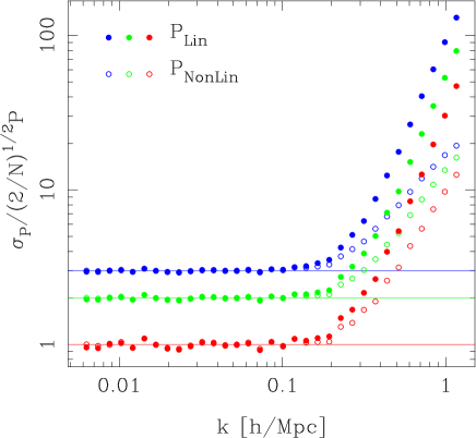
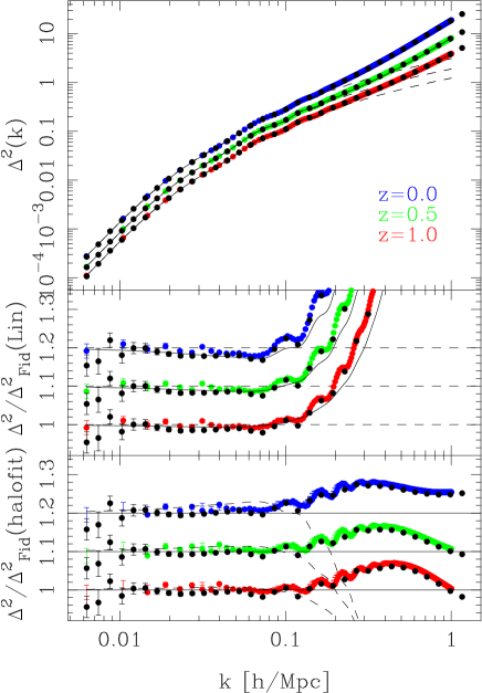
Figure 1 shows the ensemble-averaged dark matter power spectrum for the 200 realizations, at the redshifts , denoted by the green, red and blue points, respectively. The coloured points actually show the power spectra obtained from a linear binning, where the bin spacing is in units of the fundamental -cell spacing, . The black points denote the results for the 35 logarithmically spaced bins, and the error bars are on the mean. In the top panel of the figure we show the dimensionless power, which may be defined:
| (19) |
In the middle panel we show the ratio of the measured power spectra with respect to the input linear theory power spectra. For clarity, we offset the power spectra at by 20% and at by 10% in the vertical direction. The black solid line shows the nonlinear power spectra predictions from halofit (Smith et al., 2003). The plot demonstrates that strong nonlinear amplification occurs on scales , and that linear theory is not a good approximation on these scales. In addition, nonlinear amplification is not significantly weaker at higher redshifts. The bottom panel shows the ratio of the measured power spectra with respect to halofit. Again we have offset the power spectra for clarity. halofit is able to describe the measured power spectra to better than 10% on the scales investigated. The BAO wiggles appear emphasized when one takes the ratio of the nonlinear spectrum with the linear one. As was explained in (Guzik et al., 2007), this is due to the fact that the BAO in the nonlinear spectrum are damped and smoothed relative to linear, and so when one takes the ratio with the linear one sees stronger acoustic oscillations.
The shot-noise correction to the power spectrum is , which in terms of the dimensionless power is . At , this is . Thus for , the power has roughly a 10% correction, which by is reduced to 2%.
4.2 Covariance matrix
An unbiased estimator for the covariance between different band power estimates can be obtained through:
| (20) | |||||
| (21) |
where is the number of realizations.
Following Scoccimarro et al. (1999) and Smith (2009), a theoretical expression for the bin-averaged covariance matrix of the matter power spectrum, obtained from a set of densely-sampled tracers of the mass field, can be written:
| (22) |
where is the shell-averaged, connected part of the trispectrum in parallelogram configuration:
| (23) |
with being the matter trispectrum. Note that for a Gaussian random field the connected part of the trispectrum vanishes, i.e. , and the covariance reduces to:
| (24) |
Figure 2 shows the standard deviation for the matter power spectrum, i.e. , measured from the simulations, scaled in units of the square root of the Gaussian expectation for the variance given in the equation above. The figure reveals that for the diagonal errors are reasonably well described by Eq. (24). However, on smaller scales we find that the errors are significantly larger than one would expect from simple mode counting. If one uses Eq. (24) with measured from the simulations (open points in Fig. 2), then the errors appear to increase . This would suggest that in the deeply nonlinear regime as . This scaling is consistent with the predictions from the 1-Loop perturbation theory (Scoccimarro et al., 1999).
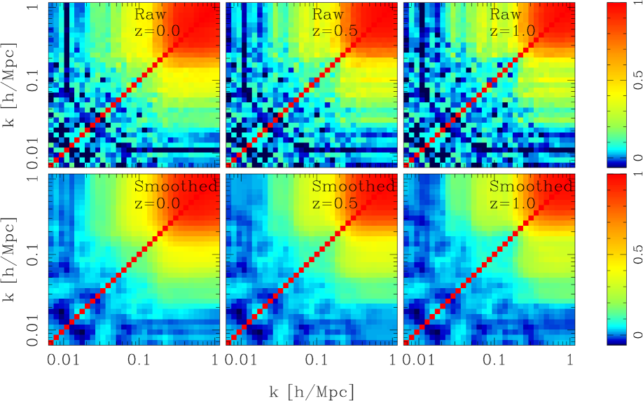
An interesting way to present the information in the off-diagonal elements of the covariance matrix is through the cross-correlation matrix. This may be defined as:
| (25) |
and it gives the strength of the covariance in a particular element relative to the square root of the product of variances in the relevant bins. It is therefore bound to the interval .
The top panels in Figure 3 present the evolution of the correlation matrix as a function of redshift from to . The increasingly redder/bluer colours demonstrate increasing/decreasing correlation strength. The results on large scales appear to be slightly noisy. The bottom panels of Fig. 3 presents the same information, only here we have performed a box-car smoothing of the correlation matrix in order to reduce the noise. For each pixel, we take the average of all pixels that are within 1-pixel from the current pixel centre, excluding the pixels on the diagonal and being careful in our treatment of the edges of the matrix. We also keep the diagonal elements fixed at (for further discussion of this approach see Mandelbaum et al., 2012). This noise reduction strategy constitutes a plausible alternative to various other ad-hoc approaches presented elsewhere in the literature (Ngan et al., 2012).
For the case of both the raw and the noise-reduced matrix, the off-diagonal correlations are in general non-zero and positive. The correlations increase as the wavenumbers of the two considered band powers are increased. Also, the correlation increases with decreasing redshift. For our choice of binning and simulation volume, we find that different power spectral band powers are correlated for at , and for by .
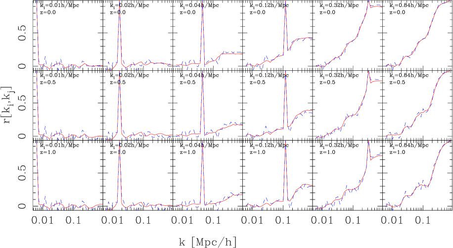
Figure 4 presents slices through the power spectrum correlation matrices measured at for the 200 realizations of the fiducial model. These results point to a reasonably good agreement between the raw and box-car-smoothed covariance matrices.
The covariance matrix of the matter power spectrum has recently been explored by Takahashi et al. (2009) who ran 5000 PM simulations in boxes of size with particles. These simulations are not of sufficiently-high spatial resolution to probe the covariance of power spectrum estimates beyond scales of the order at precision. Moreover, whilst they did employ the more accurate 2LPT initial conditions – as does our study – they also used a rather low start redshift of , which may induce small scale inaccuracies (Reed et al., 2012). On comparing their results with ours, we note that whilst they have a factor of 25 times more simulations, each of our simulations has a factor of 3 times more volume. This makes the overall difference roughly a factor of in terms of . We should therefore be able to obtain a reasonably accurate covariance matrix. This is further mitigated by our smoothing of the correlation matrix.
We also compare our study with that of Ngan et al. (2012), who used the code CUBEP3M to run 1000 simulations of boxes with and with particles. We underline that for this choice of simulation set-up, the shot-noise corrections to the power spectrum at are 6% and 30% at and , respectively. Again, whilst their study used 1000 simulations, our simulations have roughly 15 times more volume per run. Moreover, they have explored the covariance matrix for 54 bins, nearly a factor of 2 times more than we employ, hence the relative statistical power of our study should be at the very least comparable with their work. It is also worth pointing out that Ngan et al. (2012) found a 20% anti-correlation of band-powers on the largest scales. We find no evidence of such a strong anti-correlation. We also note that the power spectra from the simulations of Ngan et al. (2012) appear to show a worrying positive off-set from the linear theory predictions for the power spectrum on scales comparable to the box-scale, although this issue may now be resolved (Harnois-Deraps et al., 2012).
A more recent study by de Putter et al. (2012) has used a suite of 1024 simulations of boxes and 160 simulations of a box to explore the covariance matrix. They found that the results from the large-box simulations were in reasonably good agreement with the larger ensemble of smaller box simulations.
Thus our results are in broad agreement with all of these works and non-trivial band power correlations must be accounted for in cosmological analysis of large-scale structure data.
5 Analysis II: Variations
5.1 Power spectrum dependence on cosmological parameters
We now turn to the task of exploring the cosmological dependence of the power spectrum. As mentioned in §3, we consider the variations with respect to 7 cosmological parameters: . For each cosmological parameter, we freeze all of the other parameters and simulate two variations, up and down, around the fiducial-model value. For each such variation we have performed 4 realizations.
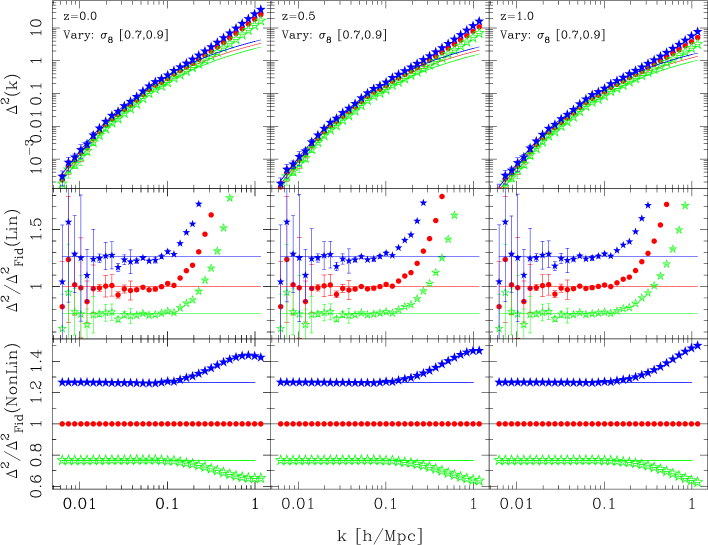
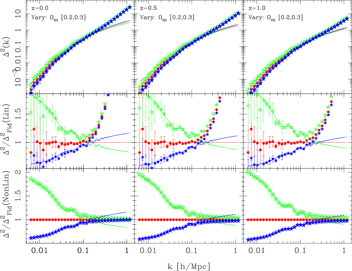
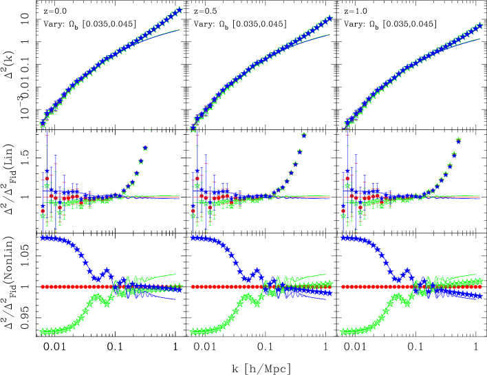
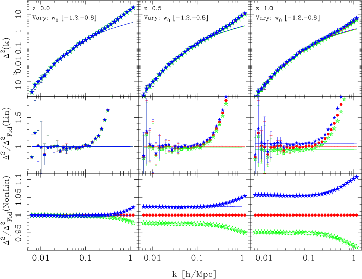
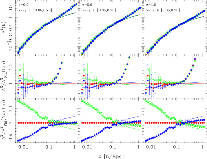
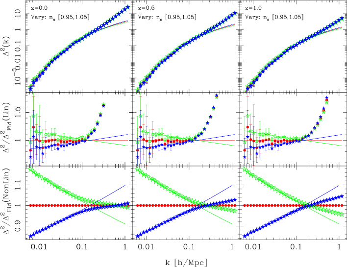
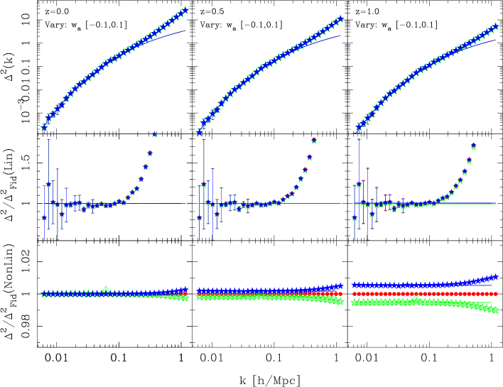
Figures 6–11 present the ensemble-averaged variations. For each figure the left, middle and right panels show the results at redshifts: , respectively. The top sections show the absolute power; the middle, the ratio with respect to the linear theory of the fiducial model; and the bottom the ratio with respect to the measured nonlinear power in the fiducial model. In all panels the red points denote the fiducial model, the blue stars denote the upper variation, i.e. , and the open green stars denote the lower variation, i.e. . It is worth noting that when we compute the ratio of the variant power spectra with the nonlinear fiducial spectrum, we compute this ratio for each realization, before averaging. This leads to the cancellation of some of the cosmic variance, and explains why the error bars in the lower sections of each panel are not visible.
We next turn our attention to the computation of the derivatives of the power spectra with respect to the cosmological parameters. In order to obtain low-noise estimates of these, we take advantage of the matched initial conditions between the variations and use the double-sided derivative estimator,
| (26) |
where for the first term on the right-hand-side we take all 200 of the fiducial simulations as described by Eq. (16). For the logarithmic derivative we use the estimator:
| (27) | |||||
where .
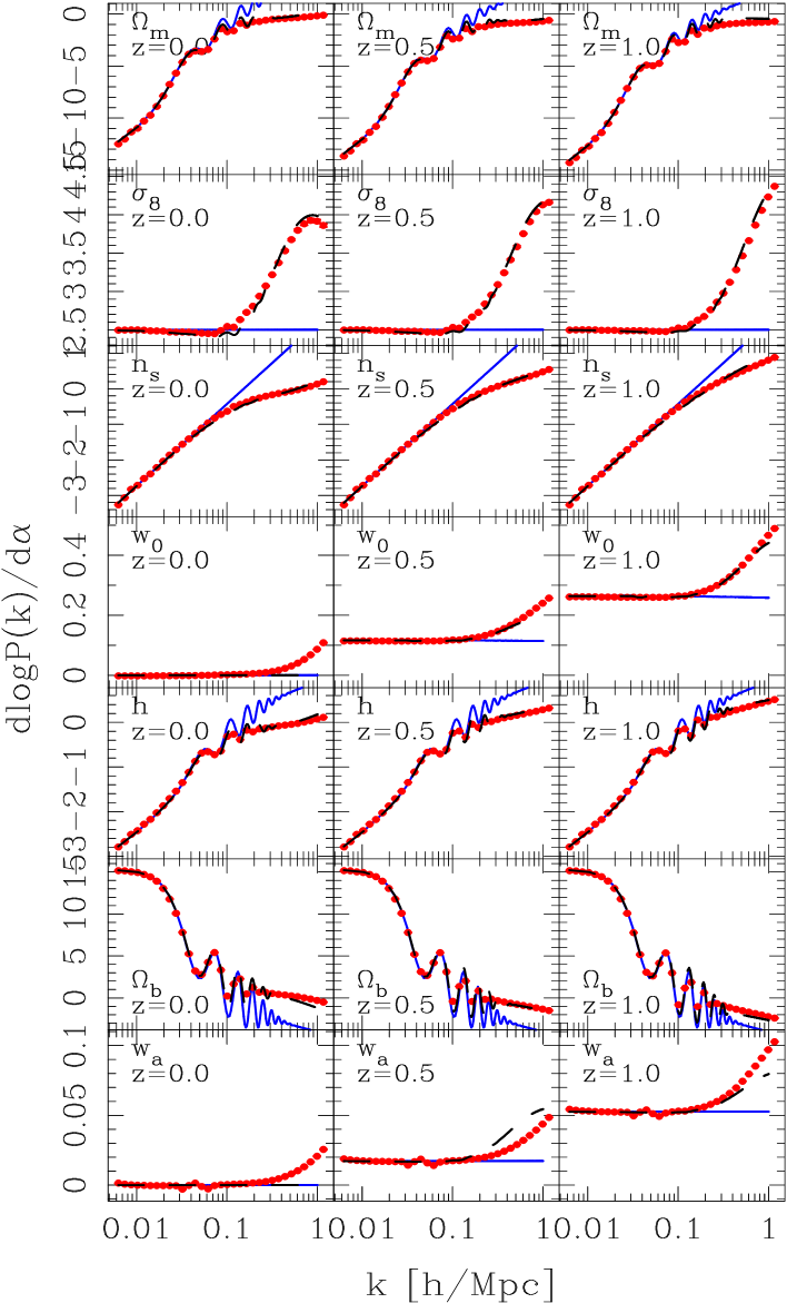
Figure 12 presents the evolution of the logarithmic derivatives of the power spectrum with respect to the 7 cosmological parameters that we have considered. The derivatives are computed as described by Eq. (27). In each panel the linear-theory derivatives are given by the solid blue lines and the black dashed lines show the predictions for the derivatives using halofit (Smith et al., 2003).
The figure demonstrates that on scales one may capture the cosmological parameter dependence of the matter power spectrum through the variations in the linear power spectrum. However, on smaller scales on must obtain the derivatives from full nonlinear modelling. With the exception of and at , the predictions from halofit are in reasonably good agreement with the estimates from the numerical simulations. For and at halofit fails to predict the nonlinear derivatives. This may partially be explained by the fact that we have normalized the initial power spectra to have the same : had we instead adopted , the amplitude of the primordial power spectrum, as our power spectrum normalization criterion, then we expect that halofit would have made more reasonable predictions (Jennings et al., 2010).
We also point out that as , the measured derivatives for appear to approach . This suggests that there is very little cosmological information to be gained by the inclusion of measurements on very small scales. On the other hand, including the information from small scales can greatly increase the cosmological information about the parameters .
5.2 Power spectrum dependence on simulation parameters
We now explore the dependence of the matter power spectrum on the Gadget-2 simulation parameters. As described in §3 we have considered variations in 9 of the parameters. As for the variations in the cosmological parameters, we take upper and lower variations of a single simulation parameter and freeze all others at their fiducial values.
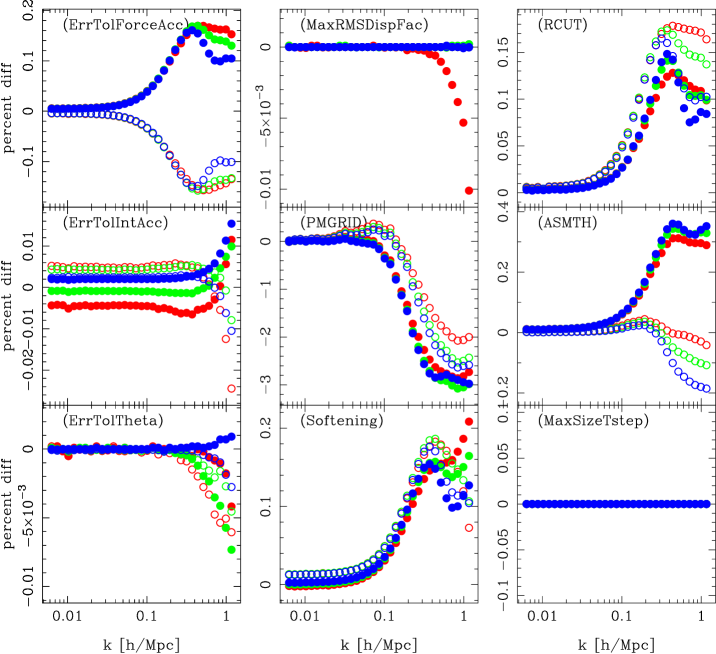
Figure 13 presents the percentage differences between the variational and the fiducial models. Each of the nine panels corresponds to one parameter, with the solid and open points depicting the upper and lower variations respectively. The blue, green and red coloured symbols show the results at epochs , respectively. We find that the most significant source of error is given by the parameter PMGRID, which can yield percent-level errors on small scales. We also find that the parameters which control the interpolation between the Tree- and the PM-force calculations, RCUT and ASMTH, can also introduce significant, but sub-percent errors. Again, these are most important on small scales. ErrTolForceAcc and the Softening can also induce errors in the power spectrum.
It is interesting to note that for the case of the parameters ErrTolForceAcc, ErrTolIntAcc, ASMTH the differences with respect to the fiducial model are almost symmetric for the positive and negative parameters steps. This suggests that these parameters are not at their converged values – it is likely that decreasing ErrTolForceAcc and ErrTolIntAcc will always lead to improved results since they control the accuracy of the integration. On the other-hand the parameters RCUT, PMGRID, and the Softening are not symmetric – this suggests that it is not so easy to understand how these parameters affect the accuracy of the simulations. For the case of PMGRID we speculate that there may be issues associated with beat coupling between the initial particle lattice – the memory of which is not lost until late times – and the Fourier mesh used to solve the Poisson equation. For the fiducial case, since the number of particles and the PMGRID were identical this effect would be minimised. As one moves to a different mesh then this effect occurs and induces an error which depends only on the absolute step size. For the case of the force softening it is well known that if one uses a softening that is either too large or too small, then the structure on the smallest scales can be damped. For the case of too small softening this occurs because hard two-body encounters can eject particles more easily from potential wells. In the case of Fig. 13 we see that the power increases for both positive and negative steps. This might be explained by the fact that if the inner-densities are decreased, then the outer edges of clusters will have an increased power amount of matter and hence an increased power spectrum. Indeed our plots do indeed show a turnover at – the turn up at higher may be due to the fact that the shot noise has not been subtracted.
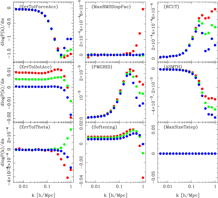
Another important point to note is that the figure also shows that all of the variations are relatively time-independent. This can be demonstrated more clearly by considering the logarithmic derivatives. Figure 14 presents the logarithmic derivatives of the matter power spectrum with respect to variations in the Gadget-2 simulation parameters. We estimate the derivatives as described by Eq. (27), except that we only use a single realization to do this. We now make some important observations: firstly, on large scales, with the exception of the parameter ErrTolIntAcc, all of the derivatives are very close to zero. Moreover, they display a very weak dependence on redshift, which is a marked difference from the cosmological parameters, which tend to evolve with both time and scale. This is an important point, suggesting that the information coming from the cosmology dependence of the simulations can be disentangled from that coming from the simulation parameters.
6 Fisher Matrix Results
Having obtained estimates for the time evolution of the fiducial model power spectrum, its covariance matrix and its derivatives with respect to the cosmological and simulation parameters, we are now in a position to explore the true cosmological information content of the power spectrum.
6.1 Estimator for the Fisher matrix
We compute the Fisher matrix as described by Eq. (15), and after dropping the first term, the estimator is:
| (28) |
We shall not use the above equation directly, but an alternate form. Consider the matrix C, and let us rewrite it as
| (29) |
(no summing over repeated indices), where is the variance associated to the th measurement bin. The inverse of C can be written as
| (30) |
Using the above identity allows us to rewrite Eq. (28) as:
| (31) |
where and . This latter form is very useful, since one simply needs to invert the correlation matrix rather than the covariance matrix. In theory there should be no difference between the results from these two approaches, however, on a computer there can be. Whilst the elements of the covariance matrix can differ wildly, even by orders of magnitude, the elements of the correlation matrix are constrained to range from . Thus we reduce the risk of inaccurate and potentially unstable inverse estimates due to round-off errors. This is especially true when large dynamic ranges are considered and when many matrix elements are employed.
6.2 Information content of the power spectrum
For our cosmological forecast we adopt a survey consisting of three independent volumes, each of which has the same volume , but mapping the three epochs . Whilst this does not directly match a particular survey, it covers the scale and evolution that should be obtainable with BOSS or DES.
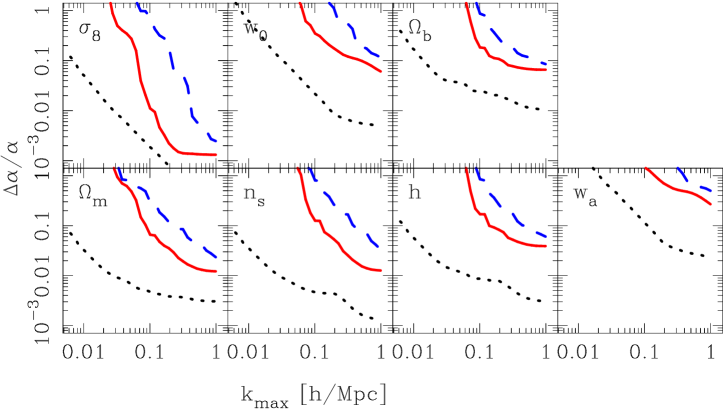
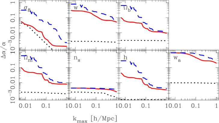
Figure 16 shows the fractional errors in the matter power spectrum for the variations in the 7 cosmological parameters, at epochs , and as a function of the maximum wavenumber that enters the calculation, i.e. . Note that since the fiducial value of , for this case we simply plot . In the figure, the unmarginalized errors on the parameters are given by the dotted black lines, i.e. . This 1- error is valid only if all the other parameters are known.
If we are required to estimate all parameters from the data then the best we can ever do is to saturate the MVB, as described in §2. If we assume that the simulation parameters are known, then the errors are given by Eq. (13), i.e. , and we obtain the solid red lines in Fig. 16. Notice that the cosmological information is significantly reduced. Once is reached, adding smaller scales does not reduce the errors on most of the parameters. This is with the exception of , and , for which adding small-scale structures does help.
On the other hand, if we are to marginalize over the simulation parameters, owing to the fact that we are ignorant as to the optimal ones, then the errors are given by Eq. (14), i.e. . These are represented in the figure by the blue dashed lines.
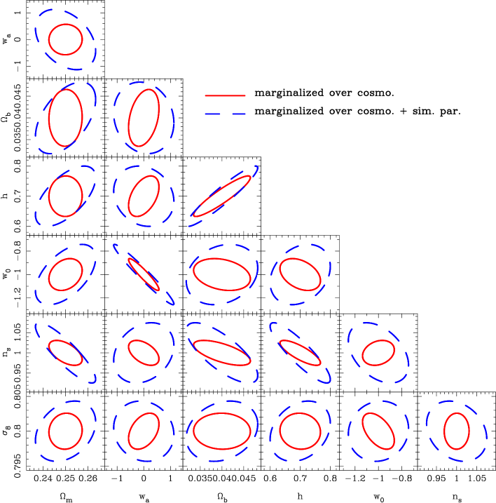
Figure 16 shows the 2D likelihood surfaces for various parameter combinations after marginalizing over all other parameters. In all of the panels we take and consider only the 2- errors, denoted by . Again the red solid lines present the results for the case where the simulation parameters are fixed and the blue dashed lines the case where we marginalize over the simulation parameters. Clearly, there would be a significant degradation in the constraining power of any future galaxy clustering survey, should we not be able to identify the ‘optimal’ simulation parameters. Note also that there appears to be a strong degeneracy between and .
6.3 Combining information from large-scale structures with the CMB
We now turn to the question of whether adding external data sets may help alleviate the degradation of the cosmological constraints. Here we only consider the impact on the errors of adding the information from a CMB experiment such as Planck (The Planck Collaboration, 2006). Note that even without Planck data we have already restricted our exploration of the cosmological parameter space to include only flat models. As described in Appendix A, we first compute the CMB Fisher matrix in a set of parameters that are suitable for the CMB, and then rotate this matrix to our favoured parameter set for describing large-scale structure (see also Hilbert et al., 2012). We treat the CMB and Large-scale structure information as independent and hence the Fisher matrices may be added:
| (32) |
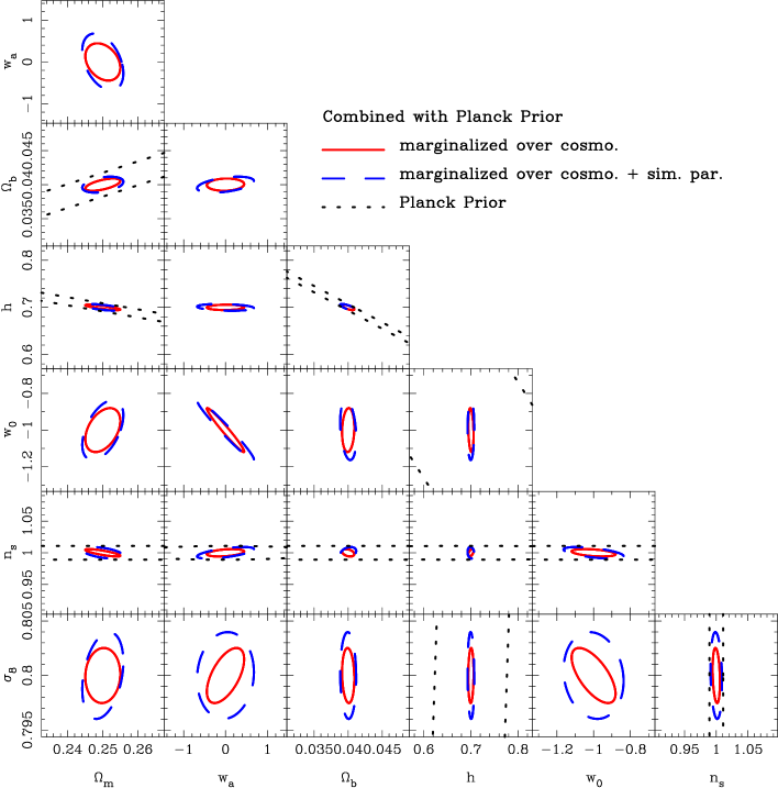
Figure 18 shows again the errors for the 7 cosmological parameters that we have considered. The differences between the errors obtained from marginalizing over the cosmological parameters (red lines) and the cosmological-plus-simulation parameters (blue lines) are significantly reduced. Thus, inclusion of the CMB information significantly improves our ability to constrain the cosmological model.
Figure 18 shows how the 95%-confidence-level error ellipses changed when we add the CMB information. We see again that the constraining power of the combined experiments significantly improves our ability to constrain cosmology, and also marginalize over the simulation parameters.
7 Constraining Dark Energy
We now turn to the question of how well we may constrain the time evolution of the dark energy equation of state, i.e. .
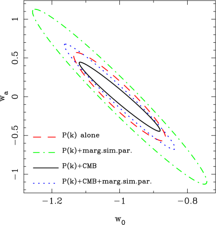
Figure 19 shows the 95%-confidence-level likelihood contours for , where we use all information from LSS up to . The figure reveals that the best constraints will come from the combination of CMB and LSS information. However, if we do not understand how to optimize our -body codes to provide ’optimal’ cosmological power spectra, then marginalizing over the simulation parameters will be costly for Dark Energy science.
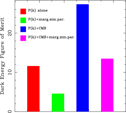
Currently, the standard way to describe the ability of an experiment to constrain is through the figure of merit (hereafter FOM) (Albrecht et al., 2006). This has been defined as the inverse area enclosed by the 2- error ellipsoid of the parameters . In terms of the Fisher matrix, this may be written:
| (33) |
where the parameter covariance matrix is the matrix formed from the submatrix of the elements of the inverse of the Fisher matrix (e.g. see Wang, 2008).
Figure 20 compares the various dark energy figures of merit. From the figure we clearly see that if one marginalizes over the simulation parameters, then there is roughly a factor of 2 penalty in our ability constrain the parameters .
8 Discussion: Validity of the Fisher matrix approach
We now discuss and emphasize some important caveats to our results.
Firstly, let us reexamine the main premise of the paper – that for a given simulation code there are parameters that if not optimally chosen should be marginalized over. One might argue that simulations do not have ‘free’ parameters, but parameters that simply control the accuracy of the numerical integration. In principle this is true, however, for a given -body algorithm it is not clear that a given code can practically satisfy this ideal statement. Consider for example the code Gadget-2, one might argue that simultaneously increasing RCUT and decreasing ErrTolTheta would lead to increasingly accurate answers – since in adopting this limit one is simply going back to computing forces with direct summation – no tree – no PM grid. However, since the tree-force is a monopole expansion and since the Ewald summation has not been implemented for the periodic boundary conditions, the code would become less accurate in the extreme limit of RCUT and ErrTolTheta=0. Even if this was implemented, then solving the forces through direct summation is not without error, since pair counts for large numbers of particles will eventually suffer from round-off errors, and Gadget-2 stores particle positions as 4-byte floating point numbers. Moreover, the order in which one takes the force sum – nearest neighbours first or distant particles first – will change the exact value of the force. We should also add that we want accurate answers from our numerical code subject to time, memory, cpu and disk usage constraints. The solution of using direct-particle summation would obviously fail the time constraint. Thus the optimization of the code parameters for Gadget-2 remains a non-trivial task.
Let us emphasize that we do not expect to have to marginalize over all simulation parameters when making cosmological inferences with real survey data – more simply put, we wish to know what would be the price one would have to pay if one failed to do the hard work to establish the ‘optimal’ set of parameters for a given algorithm – subject to the constraints mentioned above. The Fisher matrix approach offers a possible route for quickly establishing an answer to this question. It also enables us to assess at what point one can stop worrying about systematic errors in the power spectrum due to uncertainties in certain simulation parameters. For instance if the degradation in the figure-of-merit comes from a single parameter, then one can quickly identify that parameter and study its behaviour and so remove it from the marginalization step.
Another question mark concerns the use of a Gaussian posterior. It is clear that the the form of the likelihood function for obtaining a given set of measurements of the power spectrum is well described by a Gaussian. If we take the standard assumption of Gaussian initial conditions, i.e. Fourier modes are Gaussianly distributed, then the distribution of power in a given mode is exponentially distributed. If one considers the power spectrum estimator distribution, which includes the sum of modes in a given -space shell, this is -distributed (Takahashi et al., 2009). In the limit of large numbers of modes per -space shell, the -distribution becomes Gaussian. Thus it is understood that the likelihood function should be a multivariate Gaussian. However, where there is room for debate is in how one makes constraints on the cosmological parameters, at this point one needs to get an expression for the posterior probability function. Using Bayes’ theorem this is done by multiplying the likelihood by the parameter priors. Two options are possible: uninformative flat priors or if one has detailed knowledge of the system then one can write down informed priors. Since we wanted to be conservative we adopted uninformative priors. It is here where further discussion could be had, since one might argue that the parameter priors are better known. This is probably the case, however, it is worth being pessimistic at first. The functional form of the informative priors is not clear. In some cases the form of the priors is irrelevant, since as we have shown with sufficiently good data sets one can constrain certain parameters very well and so break degeneracies, e.g. is very well determined when galaxy clustering is combined with the CMB data. On the other-hand the choice of priors will most likely matter for inferences concerning the dark energy parameters.
9 Conclusions
In this paper we have used a large ensemble of -body simulations to explore the cosmological information content of the matter power spectrum. We have also explored how the cosmological information is degraded when we are uncertain as to what the ‘optimal’ -body simulation parameters are.
In §2 we introduced the ‘Gemeinsam’ likelihood function, which takes into account the dependence of the theoretical model on the cosmological and -body simulation parameters. We reviewed the Fisher matrix formalism for forecasting constraints obtainable from measurements of the matter power spectrum. The constraints required us to estimate the fiducial model power spectrum, its covariance matrix and the first order derivatives of the matter power spectrum with respect to the cosmological and simulation parameters. Our fiducial survey consisted of three independent volumes, each of which had a volume but spanning the redshifts and 1.
In §3 we described the large ensemble of simulations that we have performed in order to compute the Fisher matrix. We ran 200 simulations to generate the covariance matrix, we ran 56 simulations to explore the variations of the power spectrum with respect to the cosmological parameters; and 18 simulations to explore its dependence on the simulation parameters.
In §4 we presented the results for the fiducial model. We demonstrated that, for the errors in the power spectrum were reasonably well described by the Gaussian prediction. However, on smaller scales the errors were found to be significantly larger, and were consistent with the presence of a connected trispectrum that scaled as . We explored the off-diagonal covariance of the power spectrum and found that different band powers were correlated for at , and for by . We conclude that non-trivial band power correlations must be accounted for in the cosmological analysis of large-scale structure data.
In §5 we computed the logarithmic derivatives of the power spectrum with respect to 7 of the cosmological parameters: . We found that for the cosmological dependence could be reasonably well-captured through the variations in the linear theory spectra. On smaller scales, the measurements showed strong departures from the linear predictions. Interestingly, we found that for the parameters , and at late times, , as . This suggested that there may be very little additional cosmological information to be gained on these parameters by the inclusion of measurements on very small scales. However, we also showed that for the inclusion of small scales significantly increases the cosmological information about these parameters.
We then explored the dependence of the matter power spectrum on 9 of the simulation parameters used for the Gadget-2 code. We found that variations in the choice of PMGRID, RCUT, ASMTH, ErrTolForceAcc and Softening could in combination lead to percent-level variations in the power spectrum on small scales.
In §6 we used the simulations to explore the cosmological information content of the matter power spectrum. We found that, under the assumptions of flat cosmological models, our fiducial survey could constrain at the percent level or better, at the few-percent level and at the 20% level. However, if we fold into our likelihood analysis uncertainties in the simulation parameters then all of these constraints are degraded by roughly a factor of 2. We then showed that adding external data sets, such as a Planck-like CMB survey, can help to mitigate the effects of marginalization over the simulation parameters. In particular, the parameters are almost unaffected by the marginalization procedure.
In §7 we focused on the dark energy equation of state parameters . We have shown that marginalizing over the simulation parameters significantly degrades our ability to constrain the Dark Energy from the power spectrum. Adding the CMB information does help somewhat. However, we have computed the dark energy figure of merit and found that there is a factor of degradation when the simulation parameters are marginalized over.
In this paper we have worked with the simulation code Gadget-2 and a sub-set of parameters that are specific to it. As discussed in Reed et al. (2012), accurate simulating of cosmic structure formation involves more than the code parameters. We have neglected to explore the dependence of the information on the number of simulation particles, the box-size, the initial start redshift. Thus, taken at face value this appears to be an optimistic assessment of the problem.
On the other hand, in principle, a number of the issues raised in this paper might be mitigated by larger simulations: e.g., if one increased the number of particles without limit, then the scale at which the force softening modifies the results could be pushed to higher wavenumber, since . Hence, one could in principle find an sufficiently large that will be larger than the targeted wavemodes of the designed survey. However, finite resources may make this computationally challenging.
Regarding the generality of our conclusions, one might be concerned that the point in the simulation parameter space that we adopted as our fiducial point may bias our results and one might ask: how would the results change if we adopted another set of fiducial simulation parameters – ones closer to the optimal set? If the likelihood function does not vary rapidly over the simulation parameter space, then our estimates for the Hessian and and hence the Fisher matrix will be robust. This, however, is an important question which will deserve further attention in the future. We anticipate that answering it fully will also require one to solve the more subtle problem of finding the optimal set of simulation parameters.
This work has also focused on the problem of simulating the dark matter only power spectrum. Future work will also have to extend this analysis to include the impact of baryonic physics effects on the clustering due to: our approximate handling of the evolution of the coupled baryon-CDM fluid after recombination (Somogyi & Smith, 2010); uncertainties in the small-scale feedback processes of galaxy formation (van Daalen et al., 2011; Semboloni et al., 2011). In addition, when exploring alternative cosmological models, new uncertainties will need to be folded into the estimates for example if we also wish to constrain the dark matter model (Viel et al., 2012; Schneider et al., 2012; Bird et al., 2012).
Acknowledgements
We would like to thank the anonymous referee for their useful comments, which helped improve the quality of the draft. We also wish to thank Pablo Fosalba, Cristiano Porciani, Roman Scoccimarro, Volker Springel and Simon White for useful discussions. We kindly thank V. Springel for making public Gadget-2, and R. Scoccimarro for making public his 2LPT code. RES acknowledges support from ERC Advanced grant 246797 ‘GALFORMOD’. LM was supported by the Deutsche Forschungsgemeinschaft (DFG) through the grants MA 4967/1-1 and MA 4967/1-2. BM was supported by an SNF grant. MC was supported by the Ramòn y Cajal fellowship.
References
- Albrecht et al. (2006) Albrecht A., Bernstein G., Cahn R., Freedman W. L., Hewitt J., Hu W., Huth J., Kamionkowski M., Kolb E. W., Knox L., Mather J. C., Staggs S., Suntzeff N. B., 2006, arXiv:astro-ph/0609591
- Bernardeau et al. (2002) Bernardeau F., Colombi S., Gaztañaga E., Scoccimarro R., 2002, Phys. Rep. , 367, 1
- Bird et al. (2012) Bird S., Viel M., Haehnelt M. G., 2012, MNRAS, 420, 2551
- Crocce et al. (2006) Crocce M., Pueblas S., Scoccimarro R., 2006, MNRAS, 373, 369
- Crocce & Scoccimarro (2008) Crocce M., Scoccimarro R., 2008, PRD, 77, 023533
- de Putter et al. (2012) de Putter R., Wagner C., Mena O., Verde L., Percival W. J., 2012, Journal of Cosmology and Astro-Particle Physics, 4, 19
- Dodelson (2003) Dodelson S., 2003, Modern cosmology. Modern cosmology / Scott Dodelson. Amsterdam (Netherlands): Academic Press. ISBN 0-12-219141-2, 2003, XIII + 440 p.
- Eisenstein et al. (1999) Eisenstein D. J., Hu W., Tegmark M., 1999, ApJ, 518, 2
- Guzik et al. (2007) Guzik J., Bernstein G., Smith R. E., 2007, MNRAS, 375, 1329
- Hamilton et al. (1991) Hamilton A. J. S., Kumar P., Lu E., Matthews A., 1991, ApJL, 374, L1
- Harnois-Deraps et al. (2012) Harnois-Deraps J., Pen U.-L., Iliev I. T., Merz H., Emberson J. D., Desjacques V., 2012, ArXiv e-prints
- Heavens (2009) Heavens A., 2009, ArXiv e-prints
- Heitmann et al. (2008) Heitmann K., Lukić Z., Fasel P., Habib S., Warren M. S., White M., Ahrens J., Ankeny L., Armstrong R., O’Shea B., Ricker P. M., Springel V., Stadel J., Trac H., 2008, Computational Science and Discovery, 1, 015003
- Heitmann et al. (2005) Heitmann K., Ricker P. M., Warren M. S., Habib S., 2005, ApJS, 160, 28
- Hilbert et al. (2012) Hilbert S., Marian L., Smith R. E., Desjacques V., 2012, ArXiv e-prints
- Hu & Sawicki (2007) Hu W., Sawicki I., 2007, PRD, 76, 104043
- Jennings et al. (2010) Jennings E., Baugh C. M., Angulo R. E., Pascoli S., 2010, MNRAS, 401, 2181
- Jing (2005) Jing Y. P., 2005, ApJ, 620, 559
- Komatsu et al. (2009) Komatsu E., Dunkley J., Nolta M. R., Bennett C. L., Gold B., Hinshaw G., Jarosik N., Larson D., Limon M., Page L., Spergel D. N., Halpern M., Hill R. S., Kogut A., Meyer S. S., Tucker G. S., Weiland J. L., Wollack E., Wright E. L., 2009, ApJS, 180, 330
- Komatsu et al. (2011) Komatsu E., Smith K. M., Dunkley J., The WMAP Team 2011, ApJS, 192, 18
- Lewis et al. (2000) Lewis A., Challinor A., Lasenby A., 2000, Astrophys. J., 538, 473
- Ma & Fry (2000) Ma C., Fry J. N., 2000, ApJ, 543, 503
- Mandelbaum et al. (2012) Mandelbaum R., Slosar A., Baldauf T., Seljak U., Hirata C. M., Nakajima R., Reyes R., Smith R. E., 2012, ArXiv e-prints
- Ngan et al. (2012) Ngan W., Harnois-Déraps J., Pen U.-L., McDonald P., MacDonald I., 2012, MNRAS, 419, 2949
- Peacock & Dodds (1996) Peacock J. A., Dodds S. J., 1996, MNRAS, 280, L19
- Peacock & Smith (2000) Peacock J. A., Smith R. E., 2000, MNRAS, 318, 1144
- Peebles (1980) Peebles P. J. E., 1980, The large-scale structure of the universe. Research supported by the National Science Foundation. Princeton, N.J., Princeton University Press, 1980. 435 p.
- Press et al. (1992) Press W. H., Teukolsky S. A., Vetterling W. T., Flannery B. P., 1992, Numerical recipes in FORTRAN. The art of scientific computing. Cambridge: University Press, —c1992, 2nd ed.
- Reed et al. (2012) Reed D. S., Smith R. E., Potter D., Schneider A., Stadel J., Moore B., 2012, ArXiv e-prints
- Reyes et al. (2010) Reyes R., Mandelbaum R., Seljak U., Baldauf T., Gunn J. E., Lombriser L., Smith R. E., 2010, Nature, 464, 256
- Schneider et al. (2012) Schneider A., Smith R. E., Macciò A. V., Moore B., 2012, MNRAS, 424, 684
- Scoccimarro et al. (1999) Scoccimarro R., Zaldarriaga M., Hui L., 1999, ApJ, 527, 1
- Seljak (2000) Seljak U., 2000, MNRAS, 318, 203
- Seljak & Zaldarriaga (1996) Seljak U., Zaldarriaga M., 1996, ApJ, 469, 437
- Semboloni et al. (2011) Semboloni E., Hoekstra H., Schaye J., van Daalen M. P., McCarthy I. G., 2011, MNRAS, 417, 2020
- Smith (2009) Smith R. E., 2009, MNRAS, pp 1337–+
- Smith et al. (2003) Smith R. E., Peacock J. A., Jenkins A., White S. D. M., Frenk C. S., Pearce F. R., Thomas P. A., Efstathiou G., Couchman H. M. P., 2003, MNRAS, 341, 1311
- Smith et al. (2008) Smith R. E., Sheth R. K., Scoccimarro R., 2008, PRD, 78, 023523
- Somogyi & Smith (2010) Somogyi G., Smith R. E., 2010, PRD, 81, 023524
- Springel (2005) Springel V., 2005, MNRAS, 364, 1105
- Takada & Jain (2009) Takada M., Jain B., 2009, MNRAS, 395, 2065
- Takahashi et al. (2009) Takahashi R., Yoshida N., Takada M., Matsubara T., Sugiyama N., Kayo I., Nishizawa A. J., Nishimichi T., Saito S., Taruya A., 2009, ArXiv e-prints
- Tegmark (1997) Tegmark M., 1997, Physical Review Letters, 79, 3806
- Tegmark et al. (1997) Tegmark M., Taylor A. N., Heavens A. F., 1997, ApJ, 480, 22
- The Planck Collaboration (2006) The Planck Collaboration 2006, ArXiv Astrophysics e-prints
- van Daalen et al. (2011) van Daalen M. P., Schaye J., Booth C. M., Dalla Vecchia C., 2011, MNRAS, 415, 3649
- Viel et al. (2012) Viel M., Markovivc K., Baldi M., Weller J., 2012, MNRAS, 421, 50
- Wang (2008) Wang Y., 2008, Journal of Cosmology and Astro-Particle Physics, 5, 21
- Weinberg (2008) Weinberg S., 2008, Cosmology. Cosmology, by Steven Weinberg. ISBN 978-0-19-852682-7. Published by Oxford University Press, Oxford, UK, 2008.
Appendix A Planck Fisher matrix
A.1 Computing the CMB matrix
In computing the Planck Fisher matrix we follow the methodology described in Eisenstein et al. (1999) and for the specific implementation we follow Takada & Jain (2009). We thus assume that the CMB temperature and polarization spectra constrain 9 parameters, and for our calculations we set their fiducial values to be those from the recent WMAP7 analysis (Komatsu et al., 2011). The fiducial parameters are: dark energy EOS parameters and ; the density parameter for dark energy ; the CDM and baryon density parameters scaled by the square of the dimensionless Hubble parameter and (); and the primordial spectral index of scalar perturbations ; the primordial amplitude of scalar perturbations ; the running of the spectral index ; and the optical depth to the last scattering surface . Hence we may write our vector of parameters:
| (34) |
The CMB Fisher matrix can be written as (Eisenstein et al., 1999):
| (35) |
where , where is the temperature power spectrum, is the E-mode polarization power spectrum, is the temperature-E-mode polarization cross-power spectrum. We have been conservative and assumed that there will be no significant information from the , the B-mode polarization power spectrum. We compute all CMB spectra using CAMB (Lewis et al., 2000) and use the additional module for time evolving dark energy models (Hu & Sawicki, 2007). We include information from all multipoles in the range ().
The covariance matrices for these observables are:
| (36) | ||||
| (37) | ||||
| (38) | ||||
| (39) | ||||
| (40) | ||||
| (41) |
In the above is the fraction of sky that is surveyed and usable for science, and we take . The terms and denote the beam-noise in the temperature and polarization detectors, respectively. These can be expressed as:
| (42) | ||||
| (43) |
where and . The beam window function has the form:
| (44) |
For the Planck experiment we assume that we have a single frequency band for science (143 GHz), and for this channel the following parameters apply (The Planck Collaboration, 2006): angular resolution of the beam [FWHM]; the beam intensity is , . We take the temperature of the CMB to be .
A.2 Transforming from CMB to large-scale structure parameters
In the formation of the large-scale structure we have considered how the matter power spectrum depends on the 7 cosmological parameters: parameters. Let us rewrite our original 9-D CMB parameter set in terms of a new 9-D large-scale structure parameter set. Let us therefore consider the transformation:
| (45) | |||||
| (46) |
Five of the parameters are unchanged from the original set. The remaining four are related to the original parameters in the following way:
| (47) | |||||
| (48) | |||||
| (49) | |||||
| (50) |
where is the matter power spectrum, which depends on parameters , and where the real space, spherical top-hat filter function has the form , with and .
It can be shown that a Fisher matrix in one set of suitable variables may be represented in another basis space through the transformation:
| (51) |
where is the matrix formed from the partial derivatives of the old parameters with respect to the new ones. From Eqns (47)–(50) we have , however in order to perform the partial derivatives we actually require the inverse of these relations, i.e. . In some cases these inverse relations may easily be determined, e.g. Eq. (47). However, in other cases no analytic inverse exists, e.g. Eq. (50). A simple way around this problem is through recalling the following:
| (52) |
Hence, if we first compute , then we may obtain , from the fact that: .
Let us therefore form the matrix . For the case of those parameters that are unchanged . However, for the remaining ones, we have:
| (53) | ||||
| (54) | ||||
| (55) | ||||
| (56) | ||||
| (57) | ||||
| (58) | ||||
| (59) |
Note that in order to compute the derivatives we use the package CAMB. Besides the generation of various CMB power spectra, this package can output the present day linear theory matter power spectra . The derivatives are then determined numerically using the standard estimator for two sided derivatives. The numerical inverse of the matrix can easily be computed using the SVD algorithm (Press et al., 1992).