Stringy Pomeron:
Entropy and Shear Viscosity

Abstract

We model the soft pomeron contribution to dipole-dipole scattering as a closed string exchange in AdS₅ with a wall. The exchange of closed and long strings is characterized by an apparent Unruh temperature and entropy that are caused by the rapidity interval $\chi$ of the collision. We show that the primordial transverse shear viscosity to transverse entropy density ratio is $\eta_{\perp}/s_{\perp}=(\pi k/\chi)^{2}/8\pi$ for scattering dipoles of N-ality k, vanishing at large $\chi$.

I introduction

Collider experiments using heavy ions have revealed a novel state of hadronic matter referred to as the strongly coupled QGP (sQGP) Shuryak and Zahed (2004). This state of matter is characterized by large hadronic multiplicities and strong azimuthal particle fluctuations that appear to be well described by hydrodynamical models Shuryak (2004); Voloshin et al. (2008); Huovinen (2003); Kolb and Heinz (2003). The rapid onset of hydrodynamics with nearly ideal (shear) viscosity Molnar and Gyulassy (2002); Teaney (2003); Romatschke and Romatschke (2007); Xu et al. (2008); Xu and Greiner (2009); Drescher et al. (2007); Song and Heinz (2008); Dusling and Teaney (2008); Molnar and Huovinen (2008); Ferini et al. (2009); Danielewicz and Gyulassy (1985) points to short mean free paths and thus strong coupling. The large initial multiplicities mean very prompt and large entropy release. Theoretical models for prompt and large entropy release were discussed both at weak coupling in QCD Kharzeev et al. (2005a, b); Schenke et al. (2012); Baier et al. (2002, 2011); Fries et al. (2009) and strong coupling in holographic QCD Shuryak et al. (2007); Gubser et al. (2008); Lin and Shuryak (2009); Wu and Romatschke (2011); Kiritsis and Taliotis (2012).

Heavy ion collisions at large current colliders energies involve a large number of pp collisions with $\sqrt{s}$ ranging from $0.2-7$ TeV. pp collisions at these energies are dominated by pomeron exchanges Gribov (2002); Donnachie and Landshoff (1992). At large $N_{c}$ the pomeron is a close bosonic string Veneziano (1976). The pomeron diffusion in rapidity $\chi={\rm ln}(s/s_{0})$ also referred to as Gribov diffusion, is best captured through long strings in hyperbolic AdS space with confinement at strong coupling Janik and Peschanski (2000); Janik (2001); Basar et al. (2012). The pomeron diffusion was also thoroughly discussed in Brower et al. (2007, 2009) using a 10-dimensional supersymmetric string, both without and with confinement.

At very high energies the rapidity interval parameter $\chi$ plays the role of an effective time. For fixed momentum transfer, the string diffuses in the transverse space. The 2 transverse space coordinates need to be complemented by an additional dipole scale z-coordinate, thus $D_{\perp}=3$. Its initial value is the physical size of the colliding dipoles. This z-coordinate is not flat but hyperbolic to account for the conformal nature of QCD evolution. The diffusion means the production of small size dipoles in the transverse plane that fills the rapidity interval as detailed in Stoffers and Zahed (2013). We will refer to these diffusing dipoles as the primordial matter.

At large rapidity $\chi$, this closed string exchange is characterized by an effective Unruh temperature $1/\beta$. This temperature is caused by the emergence of a local acceleration on the string world-sheet needed to interpolate between the receding string end-points of opposite rapidities $\pm\chi/2$. The Unruh temperature $1/\beta$ is lower than the string Hagedorn temperature $1/\beta_{H}$. However, it is enough to excite the string tachyon in non-critical dimensions and therefore induce entropy. This entropy is encoded in the rapidly growing string degeneracy. Estimates show that the entropy released is about $1/3$ per dipole-dipole collisions, with about 10 dipoles per pp collisions at typical collider energies Stoffers and Zahed (2012a).

The stringy entropy released in individual pp collisions translates to a formidable prompt entropy in AA collisions under the assumption of holographic saturation Stoffers and Zahed (2013); Stoffers and Zahed (2012a). A reasonable assessment of the charged multiplicities at collider energies both at RHIC and LHC was made in Stoffers and Zahed (2012a). In particular, the stringy entropy was argued to be deposited over short time scales, typically of order $(25\,{\rm fm})/\chi^{3}$. We now suggest that the excited transverse string modes are characterized by a low viscosity that asymptotes zero at large rapidity $\chi$. This is a new result that may justify the use of nearly ideal hydrodynamics in the first $1\,{\rm fm}/c$ in the current minimum-bias collisions at collider energies. We recall that the initial jittery spatial anisotropies produced in the prompt part of the collision, can be smoothly converted to momentum anisotropies if the shear viscosity to entopy of the prompt matter is low.

In section 2 we review the set up for dipole-dipole scattering through a closed string exchange both in flat and curved space. In section 3 and 4 we argue that the transverse pomeron propagator is actually a thermal partition function for the transverse string modes with a small apparent temperature at large rapidity $\chi$. In section 5 we detail the construction of the transverse stress tensor and use it to assess the primordial shear viscosity in linear response. Our conclusions follow in section 6. The appendix details the functional and canonical quantization of the pomeron as a twisted string in flat D-dimensions.

II Dipole-Dipole Scattering

To make our discussion self-contained, we briefly review the basic formulation for the elastic dipole-dipole scattering amplitude through a Wilson loop correlator Nachtmann (1991, 1996); Korchemsky (1994); Shoshi et al. (2002) first in flat $D=2+D_{\perp}$ dimensions. Each dipole is described by a Wilson loop as shown in Fig. 1. The kinematics is captured by a fixed impact parameter ${\bf b}_{\perp}$, conjugate to the transferred momentum ${\bf q}_{\perp}$, and the rapidity interval $\chi$ related to the collisional energy. At high energies, the T-matrix factorizes Kramer and Dosch (1990); Dosch et al. (1994); Nachtmann (1996)

$${\mathcal{T}}_{12\rightarrow 34}(s,t)=2is\int du_{1}du_{2}\ \psi_{4}(u_{1})\psi_{3}(u_{1})\,{\mathcal{T}}_{DD}(\chi,{\bf q}_{\perp},u_{1},u_{2})\ \psi_{2}(u_{2})\psi_{1}(u_{2})\ ,$$ (2.0.1)

where $u_{i}$ is related to the transverse size of the dipole element described by the wave function $\psi_{i}$. The dipole-dipole scattering amplitude is given by

$${\cal T}_{DD}(\chi,{\bf q}_{\perp},u_{1},u_{2})=\int d^{D_{\perp}-1}{\bf b}_{\perp}\ e^{i{\bf q}_{\perp}\cdot{\bf b}_{\perp}}\,{\bf WW}\ ,$$ (2.0.2)

with

$${\bf WW}\equiv 1-\langle{\bf W}(C_{1}){\bf W}(C_{2})\rangle_{G}$$ (2.0.3)

The integration is taken over the $D_{\perp}-1$ dimensional impact parameter space separating the two dipoles. For the results to follow and for simplicity, the dipole sizes will be fixed to $a$ near the UV boundary. We use the normalization $\langle{\bf W}\rangle=1$ and focus only on the connected part of the correlator. The Wilson loops are evaluated along the surfaces $C_{1},C_{2}$ pictured in Fig. 1. The subscript $G$ indicates that the expectation value of the Wilson loop correlator is taken over gauge fields. This is the pomeron limit.

We note that ${\cal T}_{DD}$ in (2.0.1-2.0.2) is the closed string propagator attached to the 2 sourcing dipoles in 5-dimensions. It different is from the distorted (by curvature) spin-2 graviton exchange of Brower et al. (2007, 2009). The graviton is massive in walled AdS. Our approach is similar to the one used initially in Janik and Peschanski (2000); Janik (2001); Basar et al. (2012) with a key difference that $D_{\perp}=5$ and not 10. In the eikonal approximation, the ultrarelativistic dipole is a scalar since it moves nearly on the light cone. In (2.0.2) we have suppressed a dependence on the individual momenta of the dipole constituents and assumed that the total momentum of each dipole is equally distributed between its constituents. The effective size of the dipole is at a maximum when the momentum is unequally distributed and, hence, we are restricting our analysis to small dipoles.

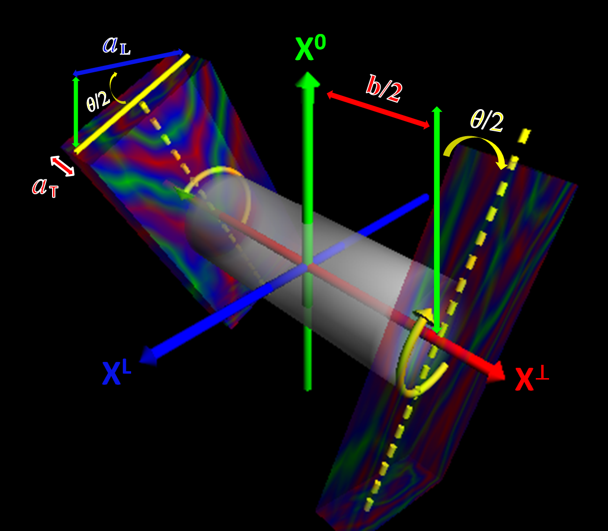
Figure 1: Twisted surface connecting the Wilson loops.

When the dipoles are small compared to the impact parameter and the rapidity interval is large, the surface connecting the two dipoles is highly twisted and can be approximated by the world-sheet of a string with the appropriate boundary conditions, see Figure 1. The exchanged surface in Figure 1 is the world-sheet surface of a closed string exchanged in the t-channel. The string is subjected to twisted (boosted) boundary conditions. The surface is best described in Euclidean space with a real twist angle $\theta$ and then analytically continued to Minkowski space through $\theta\rightarrow-i\chi$ Janik and Peschanski (2000); Janik (2001); Basar et al. (2012); Meggiolaro (1997, 1998).

At large $N_{c}$ the surface can be thought as the worldsheet made of fishnet diagrams Greensite (1985). At strong coupling $\lambda=g^{2}N_{c}$ the worlsheet can be sought in the context of holographic QCD. For that, we will use the bottom-up approach and assume the string to be exchanged in curved AdS₅ with a hard wall, i.e.

$$ds^{2}=\frac{1}{z^{2}}\left((dx^{0})^{2}+(dx^{1})^{2}+(dx_{\perp}^{2})+(dz)^{2}\right)\ ,$$ (2.0.4)

with $0\leq z\leq z_{0}$. So $D_{\perp}=3$. The holographic z-direction will be identified with the size of the probing dipoles Stoffers and Zahed (2013); Stoffers and Zahed (2012b). Their evolution is captured by the conformal nature of the AdS₅ metric in the UV. Although the field theory corresponding to this truncated space is not exactly QCD, the idea is that it captures a key aspect of the QCD string evolution in the conformal limit. A similar idea was used in the light-front translation of the holographic wavefunctions Brodsky (2007).

For dipole sizes $a$ small and near the boundary, at large impact parameters the exchanged string is long and lies mostly on the wall at $z\approx z_{0}$ whereby the metric is nearly flat Janik and Peschanski (2000); Janik (2001); Basar et al. (2012). In this limit the string action can be approximated by the flat Polyakov action

$$S[x]=\frac{\sigma_{T}}{2}\int_{0}^{T}d\tau\int_{0}^{1}\left(\dot{x}^{\mu}\dot{x}_{\mu}+x^{\prime\mu}x^{\prime}_{\mu}\right)$$ (2.0.5)

with $\dot{x}=\partial_{\tau}x$ and $x^{\prime}=\partial_{\sigma}x$. The string tension is $\sigma_{T}=1/(2\pi\alpha^{\prime})$. The Regge slope $\alpha^{\prime}$ is related to the fundamental string length by $\alpha^{\prime}=l_{s}^{2}\approx 1/(z_{0}^{2}{\sqrt{\lambda}})$. We have made the following gauge choice for the world-sheet metric $h^{a}_{b}=\delta^{a}_{b}$. With this in mind, the Wilson loop correlator is that of a closed string exchange Basar et al. (2012)

$${\bf WW}=g_{s}^{2}\int_{0}^{\infty}\frac{dT}{2T}\ {\bf K}(T)\ .$$ (2.0.6)

with the string partition function

$${\bf K}(T)=\int_{T}d[x]\ e^{-S[x]+{\rm ghosts}}\ .$$ (2.0.7)

The closed string is parametrized by one parameter, the modulus (”circumference”) $T$. The factor $g_{s}^{2}$ in (2.0.6) comes from the genus of the string configuration compared to the disconnected configuration.

Some details regarding the computation of the partition function (2.0.7) can be found in the appendix VIII. The result is

$$\mathbb{K}(T)=i\frac{a^{2}}{\alpha^{\prime}}\frac{e^{-\frac{\sigma_{T}}{2}Tb^{2}}}{2\sin(\frac{T}{2}\chi)}\times\prod_{n=1}^{\infty}\prod_{s=\pm}\frac{\sinh[\frac{T}{2}n\pi]}{\sinh[\frac{T}{2}(n\pi+is\chi)]}\times\eta^{-D_{\perp}}(\frac{iT}{2})$$ (2.0.8)

or

$$\mathbb{WW}=\frac{ig_{s}^{2}a^{2}}{4\alpha^{\prime}}\int_{0}^{\infty}\frac{dT}{T}\frac{e^{-\frac{\sigma_{T}}{2}Tb^{2}}}{\sin(\frac{T}{2}\chi)}\times\prod_{n=1}^{\infty}\prod_{s=\pm}\frac{\sinh[\frac{T}{2}n\pi]}{\sinh[\frac{T}{2}(n\pi+is\chi)]}\times\eta^{-D_{\perp}}(\frac{iT}{2})$$ (2.0.9)

with $b^{2}=\mathbb{b}_{\perp}^{2}$. The integral is dominated by the poles along the real T-axis or $T\chi/2=k\pi$ with positive integer $k$. Thus

$$\mathbb{WW}=\pi g_{s}^{2}\frac{a^{2}}{4\alpha^{\prime}}\sum_{k=1}^{\infty}\frac{\chi}{2k\pi}\frac{2}{\chi}(-1)^{k}e^{-k\frac{\pi\sigma_{T}b^{2}}{\chi}}\times\prod_{n=1}^{\infty}\prod_{s=\pm}\frac{\sinh(\frac{\pi^{2}nk}{\chi})}{\sinh[\frac{\pi^{2}nk}{\chi}+is\pi k]}\times\eta^{-D_{\perp}}(\frac{ik\pi}{\chi})$$ (2.0.10)

Using the identity

$$\prod_{s=\pm}\frac{\sinh(\frac{\pi^{2}nk}{\chi})}{\sinh[\frac{\pi^{2}nk}{\chi}+is\pi k]}=\frac{(e^{\frac{\pi^{2}nk}{\chi}}-e^{-\frac{\pi^{2}nk}{\chi}})^{2}}{(e^{\frac{\pi^{2}nk}{\chi}}e^{i\pi k}-e^{-\frac{\pi^{2}nk}{\chi}}e^{-i\pi k})*(e^{\frac{\pi^{2}nk}{\chi}}e^{-i\pi k}-e^{-\frac{\pi^{2}nk}{\chi}}e^{i\pi k})}=1$$ (2.0.11)

we obtain

$$\mathbb{WW}=\frac{g_{s}^{2}a^{2}}{4\alpha^{\prime}}\sum_{k=1}^{[N_{c}/2]}\frac{(-1)^{k}}{k}e^{-k\frac{\pi\sigma_{T}\mathbb{b}^{2}}{\chi}}\eta^{-D_{\perp}}(\frac{ik\pi}{\chi})$$ (2.0.12)

In Basar et al. (2012), the sum over the successive poles labeled by $k$ was identified with the N-ality of the Wilson-loop sourcing the close string exchange in Fig. 1. Specifically, $k=1,..,[N_{c}/2]$ for the Wilson loops or $k=1$ for $N_{c}=3$. The switch from $[\infty/2]$ to $[N_{c}/2]$ can be inferred from the occurence of the k-string tension or $k\sigma_{T}$ in the exponent of (2.0.12) (see Basar et al. (2012) for further arguments).

Inserting (2.0.12) into (2.0.2) for fixed size dipoles $u_{1}=u_{2}={\rm ln}(a/z_{0})$   Stoffers and Zahed (2013); Stoffers and Zahed (2012b), we obtain for each k-ality contribution

$$\frac{1}{-2is}{\cal T}(s,t;k)\approx{g_{s}^{2}a^{2}}\int\,d^{2}\mathbb{b}_{\perp}\,e^{i\mathbb{q}_{\perp}\cdot\mathbb{b}_{\perp}}\,{\bf K}_{T}(\beta,\mathbb{b}_{\perp};k)\,\,\,$$ (2.0.13)

where ${\bf K}_{T}$ plays the role of a transverse partition function

$${\bf K}_{T}\left(\beta,\mathbb{b}_{\perp};k\right)=e^{-\sigma_{k}\beta b/2}\,\eta^{-D_{\perp}}\left(\frac{ik}{2}\frac{\beta}{b}\right)$$ (2.0.14)

Here $\sigma_{k}=k\sigma_{T}$ and $\sigma_{T}$ is the fundamental string tension. It is important to note that the poles occur at (after restoring the dimension)

$$T=T_{k}\equiv 2k\pi/\chi$$ (2.0.15)

characterizing a periodic close loop exchange in Fig. 1. Also

$$\beta\equiv 2\pi b/\chi$$ (2.0.16)

where $1/\beta$ acts as the Unruh temperature for the close string exchange. Indeed, the string end-points are at a relative acceleration $\mathbb{a}=\chi/b$, so that the average Unruh temperature on the string world-sheet is $1/\beta=\mathbb{a}/2\pi$ Basar et al. (2012).

For $N_{c}>\lambda>1$, long strings and small Unruh temperatures in comparison to the Hagedorn temperature i.e. $\beta_{H}<\beta<b$, we will refer to ${\bf K}_{T}$ as the transverse propagator or partition function. In flat $5=2+D_{\perp}$ dimensions it follows from the scalar Polyakov action with twisted boundary conditions Basar et al. (2012); Stoffers and Zahed (2013). The effects of AdS₅ curvature will be briefly discussed below. Using the modular identity for the Dedekind eta-function or $\eta(ix)=\eta(i/x)/\sqrt{x}$ Apostol (2012), allows us to rewrite the eta-function in (2.0.14) as

$${\eta^{-D_{\perp}}\left(\frac{ik}{2}\frac{\beta}{b}\right)}= \left(\frac{k\beta}{2b}\right)^{{D_{\perp}}/2}e^{\pi D_{\perp}b/6k\beta}\times\prod_{n=1}^{+\infty}\left(1-e^{-4\pi nb/k\beta}\right)^{-D_{\perp}}$$ (2.0.17)

effectively trading $\beta/b$ with $b/\beta$ which makes the string of exponents in (2.0.17) convergent. We note that large $b$ corresponds to $\sqrt{-t}\ll\sqrt{s}$ pomeron exchange kinematics. Note that by inserting (2.0.17) into (2.0.14) and then in (2.0.13) the elastic amplitude rises with $(s/s_{0})^{1+D_{\perp}/12k}$. $D_{\perp}/12k$ is just the leading Luscher correction to the classical string contribution in flat space. Curvature corrections to this result will be briefly mentioned in section 4.

III Canonical partition function

It is physically insightful to rewrite the string of products in (2.0.17) as a trace over second quantized transverse oscillator modes, whereby the hamiltonian is the temporal Virasoro generator. For that, we note that the normal mode decomposition (see also Appendix-VIII.1) is that of an untwisted string in $D_{\perp}$ dimensions with fixed end-points. Its second quantized form follows from the standard arguments given in Arvis (1983). Specifically (see also Appendix-VIII.2)

$$x_{\perp}^{i}(\tau,\sigma)={{\bf b}^{i}_{\perp}}(\frac{\sigma}{\pi}-\frac{1}{2})+i\sqrt{2\alpha^{\prime}}\,\sum_{n\neq 0}\frac{a_{n}^{i}}{n}\,{\rm sin}(n\sigma)\,e^{-in\tau}\,\,,$$ (3.0.1)

with the transverse oscillator algebra

$$\left[a_{n}^{i},a_{m}^{j}\right]=n\,\delta^{ij}\delta_{n+m,0}$$ (3.0.2)

after rescaling $\sigma\rightarrow\sigma/\pi$ for convenience. From ( 8.2.27)

$${\bf Z}_{\perp}(\beta_{k})\equiv\prod_{n=1}^{+\infty}\left(1-e^{-(4\pi b/{k\beta})\,n}\right)^{-D_{\perp}}={\rm Tr}\left(e^{-\beta_{k}\,{\bf L}_{0}}\right)$$ (3.0.3)

where $\beta_{k}=4\pi b/k\beta$ and the temporal Virasoro generator ${\bf L}_{0}$ Arvis (1983) reads

$${\bf L}_{0}=\sum_{n=1}^{\infty}\sum_{i=1}^{D_{\perp}}\,:a_{-n}^{i}a_{n}^{i}:=\sum_{n=1}^{\infty}\sum_{i=1}^{D_{\perp}}\,a_{-n}^{i}a_{n}^{i}$$ (3.0.4)

with $a_{n}\left|0\right>=0$ for $n>0$. The transverse partition function has the inspiring form of a thermal sum

$${\bf K}_{T}\left(\beta,{\bf b}_{\perp};k\right)=\left(\frac{2\pi}{\beta_{k}}\right)^{D_{\perp}/2}e^{-\sigma_{k}\beta b/2}\,{\rm Tr}\left(e^{-\beta_{k}\,\left({\bf L}_{0}-\frac{D_{\perp}}{24}\right)}\right)$$ (3.0.5)

We recall that the normal ordering of (3.0.4) produces the zero-point contribution of $D_{\perp}/24$ in (3.0.5) Arvis (1983).

Since

$$\partial_{\chi}\mathbb{K}_{T}(\beta,b;k) = [\frac{k\sigma_{T}\pi b^{2}}{\chi^{2}}-\frac{D_{\perp}}{2\chi}-\frac{2}{k}(\mathbb{L}_{0}-\frac{D_{\perp}}{24})]\mathbb{K}_{T}(\beta,b;k)$$

$$\nabla_{\perp}^{2}\mathbb{K}_{T}(\beta,b;k) = [4k\sigma_{T}\pi(\frac{k\sigma_{T}\pi}{\chi^{2}}b^{2}-\frac{D_{\perp}}{2\chi})]\mathbb{K}_{T}(\beta,b;k)$$ (3.0.6)

${\bf K}_{T}$ obeys a diffusion equation in rapidity

$$\left(\partial_{\chi}+{\bf D}_{k}\left({\bf M}_{0}^{2}-\nabla_{\bf b_{\perp}}^{2}\right)\right){\bf K}_{T}=0$$ (3.0.7)

This is the famed Gribov diffusion for the pomeron in our case viewed as the exchange of a closed string. The pomeron diffusion constant is ${\bf D}_{k}=\alpha^{\prime}/2k$. Note that

$${\bf M}^{2}_{0}=\frac{4}{\alpha^{\prime}}\left(\left<{\bf L}_{0}\right>-\frac{D_{\perp}}{24}\right)$$ (3.0.8)

is the string tachyonic mass. The average $\left<\cdots\right>$ is taken in the equilibrium thermal ensemble. While the tachyon is a liability in a potential calculation as it signals the instability of the string ground state except in critical dimensions, it is a blessing in the scattering amplitude as it is identified with the positive pomeron intercept. The averaging in (3.0.8) is carried through

$$\left<{\bf L}_{0}\right>=-\frac{\partial{\rm ln}{\bf Z}_{\perp}}{\partial\beta_{k}}={\rm Tr}\left({\bf L}_{0}\frac{e^{{-\beta_{k}}{\bf L}_{0}}}{{\bf Z}_{\perp}}\right)=D_{\perp}\sum_{n=1}^{\infty}\frac{n}{e^{{\beta_{k}}n}-1}$$ (3.0.9)

as per the diffusion equation (3.0.7). Note that since $\beta_{k}=2\chi/k$ is large, the mean occupation of the transverse string modes contributing to (3.0.9) is small

$$\left<:a_{-n}^{i}a_{n}^{i}:\right>=\frac{n}{e^{{\beta_{k}}n}-1}\approx n\,e^{-\beta_{k}n}$$ (3.0.10)

A large rapidity interval freezes the stringy pomeron exchange to its lowest tachyonic mode.

In so far most of the analysis was carried for fixed but small dipoles $a$ and large impact parameters $\mathbb{b}_{\perp}$, to take advantage of the nearly flat induced metric around $z\approx z_{0}$. While we do not know how to address quantum strings in curved AdS₅ in general, we still can assess the effects of the AdS₅ curvature on the diffusion equation (3.0.7). Indeed, by identifying the z-coordinate in (3.0.7) with the dipole size (also the size of the close string exchange), we can trade the flat Laplacian $\nabla^{2}_{\bf b_{\perp}}$ with its analogue in curved AdS${}_{D_{\perp}=3}$. The result is a diffusive equation in AdS${}_{D_{\perp}=3}$ with a $1/\sqrt{\lambda}$ correction to the tachyon mass Stoffers and Zahed (2013).

IV Entropy

The free energy associated to the transverse pomeron propagator can be identified with ${\bf F}_{k}=-{\rm ln}{\bf K}_{T}/\beta$ thanks to the induced Unruh temperature $1/\beta$. This translates to a pomeron entropy ${\bf S}_{k}=\beta^{2}\partial{\bf F}_{k}/\partial\beta$. Explicitly

$${\bf S}_{k} = \ln\mathbb{K}_{T}-\frac{\partial\ln\mathbb{K}_{T}}{\partial\ln\beta}=\ln\mathbb{K}_{T}+\frac{\partial\,{\rm ln}\mathbb{K}_{T}}{\partial\ln\chi}$$

$$= D_{\perp}\sum_{n=1}^{\infty}{\rm ln}\left(1+\frac{1}{e^{\beta_{k}n}-1}\right)+\beta_{k}\left(\frac{D_{\perp}}{12}-\left<{\bf L}_{0}\right>\right)-\frac{D_{\perp}}{2}\left(1+{\rm ln}\left(\frac{\beta_{k}}{2\pi}\right)\right)$$

Again, since $\beta_{k}=2\chi/k$ is large, (IV) is dominated by the tachyon contribution ${\bf S}_{k}\approx D_{\perp}\beta_{k}/12$  Stoffers and Zahed (2012a). Therefore, the released pomeron entropy per transverse area for large $\chi$ is

$$s_{\perp}\equiv\frac{{\bf S}_{k}}{A_{\perp}}\approx\frac{\chi}{A_{\perp}}\frac{D_{\perp}}{6k}\equiv\frac{2\,{\rm ln}{{\bf N}_{\rm wee}}}{A_{\perp}}$$ (4.0.2)

${\bf N}_{\rm wee}=e^{\chi(\alpha_{\bf P,1}-1)}$ with $\alpha_{\bf P,1}-1\approx D_{\perp}/12k$ is the number of transverse wee dipoles Stoffers and Zahed (2012a) with $(\alpha_{\bf P,1}-1)$ the (bare) pomeron intercept. The last idensity confirms our interpretation of the primordial matter as the number of wee dipoles undergoing Gribov diffusion in the transverse plane. The role of AdS₅ curvature on the exchanged string translates to $1/\sqrt{\lambda}$ corrections to (4.0.2) as detailed in Stoffers and Zahed (2012a). They correct the pomeron intercept and entropy (IV). A similar curvature correction to the pomeron as a graviton exchange in 10 dimensions was originally obtained in Brower et al. (2007, 2009).

Note that $\beta>\beta_{H}$ translates to a rapidity bound $\chi<2$ in the diffusive limit $\left<b^{2}\right>=D_{k}\chi$. A refined bound including $1/\lambda$ corrections in the pomeron intercept, is Stoffers and Zahed (2013); Stoffers and Zahed (2012a)

$$\beta>\sqrt{2(\alpha_{\bf P,1}-1)}\,\beta_{H}$$ (4.0.3)

leading to $\chi<10$ for a physical pomeron intercept of 0.08. Strings with $\chi>10$ need a resummation of the $\beta_{H}/\beta$ contributions which is beyond the scope of the scalar Polyakov action.

V Transverse shear viscosity

For the transport properties associated to the stringy modes in the transverse 3-dimensional plane to the dipole-dipole collision at large rapidity $\chi$, the transverse string modes are dominant. Their transport properties such as the transverse shear viscosity $\eta_{\perp}$ for instance, can be defined using standard linear response analysis with the density matrix $e^{-\beta_{k}{\bf L}_{0}}/{\bf Z}_{\perp}$ as defined in (3.0.9). Specifically

$$\eta_{\perp}=\lim_{\omega\rightarrow 0^{+}}\frac{1}{2\omega}\int dtd\mathbb{x}\,e^{i\omega t}\left<[T_{\perp}(t,\mathbb{x}),T_{\perp}(0,0)]\right>$$ (5.0.1)

where $T_{\perp}(t,\mathbb{x})$ is the stress tensor associated to the Polyakov string in D-dimensions. It is sufficient to consider

$$T_{\perp}(t)=\frac{1}{A_{\perp}}\int\prod^{4}_{a=1}dx^{a}\,\,T_{\perp}(t,\mathbb{x})$$ (5.0.2)

The averaging in (5.0.2) over the transverse coordinates $x^{1,2,3}$ picks the zero momentum component of of the transverse energy momentum tensor in our physical 3-dimensional space with $A_{\perp}\approx(\chi\alpha^{\prime})\,l_{s}$ Basar et al. (2012); Stoffers and Zahed (2013). Eq. 5.0.1 simplifies

$$\eta_{\perp}=\lim_{\omega\rightarrow 0^{+}}\frac{A_{\perp}}{2\omega}\int dte^{i\omega t}\left<[T_{\perp}(t),T_{\perp}(0)]\right>$$ (5.0.3)

The stress tensor associated to the Polyakov string reads

$$T^{\mu\nu}_{D}(y)=\frac{\delta S[x]}{\delta g_{\mu\nu}(y)}$$ (5.0.4)

using the Polyakov action (8.0.2). Explicitly

$$T^{\mu\nu}_{D}(y)=\frac{\sigma_{T}}{2}\int_{0}^{T}d\tau\int_{0}^{\pi}d\sigma\,\partial x^{\mu}\,\partial x^{\nu}\,\delta_{D}(x-y)$$ (5.0.5)

where $\delta_{D}(x-y)=\delta(x^{0}-y^{0})\delta(\mathbb{x}-\mathbb{y})$. We dropped the boundary contributions as they do not affect the evaluation of the transverse transport coefficient. For the transverse spatial components $\mu,\nu=i,j=2,3$ we identify the time $x^{0}=t=\tau$ with the affine coordinate on the world-sheet defined with flat metric $h=(1,-1)$. Therefore

$$\int d\tau\delta(x^{0}-y^{0})=1$$ (5.0.6)

so that

$$T^{ij}_{\perp}(\tau) = \frac{1}{A_{\perp}}\int\prod^{4}_{a=1}dy^{a}\,\,T_{\perp}^{ij}(y)$$ (5.0.7)

$$= \frac{\sigma_{T}}{2A_{\perp}}\int_{0}^{\pi}\,d\sigma\,\left(\dot{x}_{\perp}^{i}\,\dot{x}_{\perp}^{j}-{x^{\prime}}_{\perp}^{i}{x^{\prime}}_{\perp}^{j}\right)$$

Inserting (3.0.1) into (5.0.7), we obtain

$$T^{ij}_{\perp}(\tau) = (2\alpha^{\prime})\frac{\sigma_{T}}{2A_{\perp}}\int_{0}^{\pi}~{}d\sigma\sum_{n\neq 0}\sum_{n^{\prime}\neq 0}a_{n}^{i}a_{n^{\prime}}^{j}(\sin(n\sigma)\sin(n^{\prime}\sigma)e^{-i(n+n^{\prime})\tau}+\cos(n\sigma)\cos(n^{\prime}\sigma)e^{-i(n+n^{\prime})\tau})$$ (5.0.8)

$$= \frac{1}{2A_{\perp}}\sum_{n\neq 0}a_{n}^{i}a_{n}^{j}e^{-i2n\tau}$$

Pluging (5.0.8) into (5.0.3) and normal ordering yields

$$\eta_{\perp} = \lim_{\omega\to 0^{+}}\frac{A_{\perp}}{2\omega}\int_{0}^{\infty}d\tau e^{i\omega\tau}\left<:\left[T_{\perp}^{23}(\tau),T_{\perp}^{23}(0)\right]:\right>$$

$$= \lim_{\omega\to 0^{+}}\frac{A_{\perp}}{2\omega}\int_{0}^{\infty}d\tau e^{i\omega\tau}\frac{1}{4A_{\perp}^{2}}\sum_{n\neq 0}e^{-i2n\tau}n(\left<:a_{n}^{2}a_{-n}^{2}:\right>+\left<:a_{-n}^{3}a_{n}^{3}:\right>)$$

$$= \lim_{\omega\to 0^{+}}\frac{-i}{2\omega A_{\perp}}\int_{0}^{\infty}d\tau e^{i\omega\tau}\sum_{n=1}^{\infty}\frac{n^{2}}{e^{\beta_{k}n}-1}\,{\rm sin}(2n\tau)$$

Switching the summation and integration yields

$$\eta_{\perp}=\lim_{\omega\to 0^{+}}\frac{1}{4\omega A_{\perp}}\sum_{n=1}^{\infty}\,\frac{n^{2}}{e^{\beta_{k}n}-1}2\pi\delta(\omega-2n)=\frac{1}{A_{\perp}}\frac{\pi}{8\beta_{k}}$$ (5.0.10)

where the last equality follows by taking the limit after enforcing the sum. Unlike the entropy density (4.0.2), the transverse mode contributions to (5.0.10) decrease with the rapidity interval. Since the transverse string area is $A_{\perp}\approx(\chi\alpha^{\prime})\,l_{s}$, it follows that

$$\eta_{\perp}\approx\frac{\sigma_{k}}{2}\left(\frac{\pi}{2\chi}\right)^{2}$$ (5.0.11)

which is asymptotically small. The ratio of the primordial transverse viscosity (5.0.10) to transverse entropy (4.0.2) is independent of the way we set the transverse diffusion area $A_{\perp}$,

$$\frac{\eta_{\perp}}{s_{\perp}}=\frac{3\pi k^{2}}{8\chi^{2}D_{\perp}}\equiv\frac{1}{8\pi}\left(\frac{\pi k}{\chi}\right)^{2}$$ (5.0.12)

We recall that for the holographic pomeron $D_{\perp}=3$. We note that the ratio jumps by 4 in trading $k=1$ or a fundamental dipole source with $k=2$ or an adjoint dipole source. (5.0.12) is remarkable as it shows that the ratio is vanishingly small at large rapidity.

VI Conclusion

In holographic QCD the pomeron exchange in dipole-dipole scattering with a large rapidity $\chi$ is described by the exchange of a non-critical string in hyperbolic $D=5$ dimensions. The extra curved direction is identified with the dipole size. A finite rapidity interval induces a local Unruh temperature on the string world-sheet $1/\beta={\bf a}/2\pi=\chi/2\pi b$, which is at the origin of a primordial entropy Stoffers and Zahed (2012a). This Unruh temperature is due to the collision kinematics and is distinct from the dynamical Unruh temperature argued in Kharzeev (2006); Castorina et al. (2007) using the saturation momentum.

As the Unruh temperature is smaller than the Hagedorn temperature, this primordial entropy is mostly carried by the tachyonic string mode. The transverse string modes are excited, but their contribution to the transverse entropy is sub-leading at large rapidity $\chi$. However, the transverse string modes are the dominant contributors to the transverse energy momentum tensor and therefore their fluctuations dominate the transverse transport properties of this form of prompt and primordial matter released through the inelastic part of the exchange.

The transverse shear viscosity of the primordial matter released by the exchange of the pomeron over its transverse diffusive size $A_{\perp}\approx(\chi\alpha^{\prime})\,l_{s}$ is found to be small, i.e. $\eta_{\perp}\approx 1/\chi^{2}$. Unlike the transverse entropy density which is constant over the rapidity interval, the transverse viscosity is not. As a result, the ratio of the primordial transverse viscosity to transverse entropy per unit area (5.0.12) is found to vanish asymptotically.

This limit evades the $1/4\pi$ lower bound Kovtun et al. (2005) as it involves the exchange of a string that is not yet dual to a black-hole. While the transverse entropy is dominated by the tachyon and scales with the rapidity interval, the shear viscosity is due to the transverse modes which are suppressed by the rapidity interval. The transverse modes are kinematically subdominant in bulk but dominant in transverse transport. This dichotomy is the essence of the dynamical calculation we have detailed, which may well be the lore at current collider energies in the primordial stage and for the minimum bias multiplicities.

When the Unruh temperature becomes comparable to the Hagedorn temperature or $\beta\approx\beta_{H}$, the use of the scalar Polyakov action is no longer valid. A recent analysis using the Nambu-Goto action shows that the exchanged pomeron becomes explosive and dual to a black-hole with a viscosity to entropy ratio of $1/4\pi$ Shuryak and Zahed (2013a, b); Kalaydzhyan and Shuryak (2014). Explosive pomerons maybe important for the recently reported high multiplicity events in colliders Abelev et al. (2013); Aad et al. (2013).

VII Acknowledgements

We would like to thank Gokce Basar, Dima Kharzeev, Edward Shuryak, Alexander Stoffers and Derek Teaney for discussions. This work was supported by the U.S. Department of Energy under Contract No. DE-FG-88ER40388.

VIII Appendix

In this Appendix, we derive the string partition function (Eq. 2.0.8) in Sec-II by using $\mathbb{(1)}$ the functional approach and $\mathbb{(2)}$ the canonical approach. Both approaches are complementary in illustrating the appearance of thermal effects. The string partition function reads

$${\bf K}(T)=\int_{T}d[x]\ e^{-S[x]+{\rm ghosts}}$$ (8.0.1)

where

$$S[x]=\frac{\sigma_{T}}{2}\int_{0}^{T}d\tau\int_{0}^{1}d\sigma\left(\dot{x}^{\mu}\dot{x}_{\mu}+x^{\prime\mu}x^{\prime}_{\mu}\right)$$ (8.0.2)

is the Polyakov string action. The collision set up is shown in Fig. 1, with the twisted boundary conditions

$$\cos(\frac{\theta}{2})x^{1}+\sin(\frac{\theta}{2})x^{0}~{}~{}~{}|_{\sigma=0}=0,\ \ \ \ \ \ \ \ x^{\perp}|_{\sigma=0}=-\frac{\mathbb{b}^{\perp}}{2}$$

$$\cos(\frac{\theta}{2})x^{1}-\sin(\frac{\theta}{2})x^{0}~{}~{}~{}|_{\sigma=1}=0,\ \ \ \ \ \ \ \ x^{\perp}|_{\sigma=1}=+\frac{\mathbb{b}^{\perp}}{2}$$ (8.0.3)

with ${\bf b}^{\perp}=(0,\cdots,b,\cdots,0)$ and periodicity $x^{\mu}(\tau)=x^{\mu}(\tau+T)$. This latter property is at the origin of the thermal effects and the appearance of an Unruh temperature.

VIII.1 Functional approach

In Euclidean space, the twisted boundary condition (Eq. VIII) can be simplified by the following transformation

$$\begin{pmatrix}x^{0}\\ x^{1}\end{pmatrix}=\begin{pmatrix}\cos\frac{\theta_{\sigma}}{2}&-\sin\frac{\theta_{\sigma}}{2}\\ \sin\frac{\theta_{\sigma}}{2}&\cos\frac{\theta_{\sigma}}{2}\end{pmatrix}\begin{pmatrix}\tilde{x}^{0}\\ \tilde{x}^{1}\end{pmatrix}$$ (8.1.4)

with $\theta_{\sigma}=\theta(2\sigma-1)$ and leading to an ordinary Dirichlet boundary condition

$$\tilde{x}^{1}~{}~{}|_{\sigma=0,1}=0$$ (8.1.5)

Note that (8.1.5) translates to

$$\partial_{\tau}\tilde{x}^{1}~{}~{}|_{\sigma=0,1}=0\ \ \ \ \ \ \ \ \ \partial_{\sigma}\tilde{x}^{0}~{}~{}|_{\sigma=0,1}=0$$ (8.1.6)

The second equation follows from the fact that the world-sheet $T^{\alpha\beta}=\delta S/\delta h_{\alpha\beta}=0$. Thus, the mode decomposition

$$\tilde{x}^{0}(\tau,\sigma) = \sum_{m=-\infty}^{\infty}\sum_{n=0}^{\infty}y_{m,n}^{0}\exp({i2\pi m\frac{\tau}{T}})\cos(\pi n\sigma)$$

$$\tilde{x}^{1}(\tau,\sigma) = \sum_{m=-\infty}^{\infty}\sum_{n=1}^{\infty}y_{m,n}^{1}\exp({i2\pi m\frac{\tau}{T}})\sin(\pi n\sigma)$$

$$\tilde{x}^{\perp}(\tau,\sigma) = x^{\perp}(\tau,\sigma)=(\sigma-\frac{1}{2})\mathbb{b}^{\perp}+\sum_{m=-\infty}^{\infty}\sum_{n=1}^{\infty}y_{m,n}^{\perp}\exp({i2\pi m\frac{\tau}{T}})\sin(\pi n\sigma)$$ (8.1.7)

Using the above results, we can recast (8.0.1) into

$$\mathbb{K}=\mathbb{K}_{0L}\times\mathbb{K}_{\O L}\times\mathbb{K}_{\perp}\times\mathbb{K}_{\rm ghost}$$ (8.1.8)

where $\mathbb{K}_{0L}$ and $\mathbb{K}_{\O L}$ are the longitudinal zero and non-zero mode contributions respectively, $\mathbb{K}_{\perp}$ is the transverse contribution, and $\mathbb{K}_{\rm ghost}$ is the ghost contribution. The explicit forms are given by

$$\mathbb{K}_{0L}=\prod_{m=-\infty}^{\infty}[\frac{\sigma_{T}T}{2\pi}(\theta^{2}+\frac{4\pi^{2}m^{2}}{T^{2}})]^{-\frac{1}{2}}$$ (8.1.9)

$$\mathbb{K}_{\not{0}L}=\prod_{n=1}^{\infty}\prod_{s=\pm}\prod_{m=-\infty}^{\infty}\{\frac{\sigma_{T}T}{4\pi}[\frac{4m^{2}\pi^{2}}{T^{2}}+(n\pi+s\theta)^{2}]\}^{-\frac{1}{2}}$$ (8.1.10)

$$\mathbb{K}_{\perp}=\exp[-\frac{\sigma_{T}}{2}Tb^{2}]\prod_{n=1}^{\infty}\prod_{m=-\infty}^{\infty}[\frac{\sigma_{T}T}{4\pi}(\frac{4\pi^{2}m^{2}}{T^{2}}+n^{2}\pi^{2})]^{-\frac{D_{\perp}}{2}}$$ (8.1.11)

and the ghost contribution tags to the two longitudinal non-zero mode contribution

$$\mathbb{K}_{\rm ghost}=\prod_{n=1}^{\infty}\prod_{m=-\infty}^{\infty}\frac{\sigma_{T}T}{4\pi}(\frac{4m^{2}\pi^{2}}{T^{2}}+n^{2}\pi^{2})$$ (8.1.12)

The products are divergent, but can be done with the help of $\zeta$-function regularization and the product formula for $\sinh$

$$\frac{\sinh x}{x}=\prod_{n=1}^{\infty}(1+\frac{x^{2}}{\pi^{2}n^{2}})$$ (8.1.13)

The transverse-mode contribution $\mathbb{K}_{\perp}$ (Eq. 8.1.11) now reads

$$\mathbb{K}_{\perp} = \exp[-\frac{\sigma_{T}}{2}Tb^{2}]\prod_{n=1}^{\infty}\prod_{m=-\infty}^{\infty}[m^{2}(1+\frac{(\frac{n\pi T}{2})^{2}}{m^{2}\pi^{2}})]^{-\frac{D_{\perp}}{2}}$$ (8.1.14)

$$= \exp[-\frac{\sigma_{T}}{2}Tb^{2}]\prod_{n=1}^{\infty}[2\sinh(\frac{n\pi T}{2})]^{-D_{\perp}}$$

where we used $\prod_{-\infty}^{\infty}c=1$ and $\prod_{m=1}^{\infty}m=\sqrt{2\pi}$. We further notice

$$\prod_{n=1}^{\infty}2\sinh(\pi\frac{T}{2}n) = \prod_{n=1}^{\infty}(e^{\pi n\frac{T}{2}}-e^{-\pi n\frac{T}{2}})$$ (8.1.15)

$$= e^{\sum_{n=1}^{\infty}\pi n\frac{T}{2}}*\prod_{n=1}^{\infty}(1-e^{-\pi nT})$$

$$= e^{-\pi\frac{T}{24}}*\prod_{n=1}^{\infty}(1-e^{-\pi nT})$$

$$= \eta(\frac{iT}{2})$$

where $\eta(\tau)$ is Dedekind eta function after using $\zeta(0)=-1/12$. Similar arguments yield

$$\mathbb{K}_{0L} = \frac{1}{2\sinh(\frac{T}{2}\theta)}$$

$$\mathbb{K}_{\not{0}L} = \prod_{n=1}^{\infty}\prod_{s=\pm}\frac{1}{2\sinh[\frac{T}{2}(n\pi+s\theta)]}$$ (8.1.16)

In sum, the string partition function is given by

$$\mathbb{K}(T)=\frac{a^{2}}{\alpha^{\prime}}\frac{e^{-\frac{\sigma_{T}}{2}Tb^{2}}}{2\sinh(\frac{T}{2}\theta)}\times\prod_{n=1}^{\infty}\prod_{s=\pm}\frac{\sinh[\frac{T}{2}n\pi]}{\sinh[\frac{T}{2}(n\pi+s\theta)]}\times\eta^{-D_{\perp}}(\frac{iT}{2})$$ (8.1.17)

with

$$a^{2}\longrightarrow a_{T}^{2}+\frac{a_{L}^{2}}{\sin^{2}(\frac{\theta}{2})}\approx a_{T}^{2}$$ (8.1.18)

the transpose dipole size squared. The analytical continuation to Minkowski space or $\theta\longrightarrow-i\chi$, gives the final result

$$\mathbb{K}(T)=i\frac{a^{2}}{\alpha^{\prime}}\frac{e^{-\frac{\sigma_{T}}{2}Tb^{2}}}{2\sin(\frac{T}{2}\chi)}\times\prod_{n=1}^{\infty}\prod_{s=\pm}\frac{\sinh[\frac{T}{2}n\pi]}{\sinh[\frac{T}{2}(n\pi+is\chi)]}\times\eta^{-D_{\perp}}(\frac{iT}{2})$$ (8.1.19)

which is (2.0.8) as discussed in Sec-II using the functional approach.

VIII.2 canonical approach

In this subsection, we re-derive the string partition function (2.0.8) using the canonical approach. In Minkowski space, we recall the second quantized transverse coordinates (Eq. 3.0.1)

$$x_{\perp}^{i}(\tau,\sigma)={{\bf b}^{i}}(\frac{\sigma}{\pi}-\frac{1}{2})+i\sqrt{2\alpha^{\prime}}\sum_{n\neq 0}\frac{a_{n}^{i}}{n}\,{\rm sin}(n\sigma)\,e^{-in\tau}$$ (8.2.20)

with the transverse oscillator algebra

$$\left[a_{n}^{i},a_{m}^{j}\right]=n\,\delta^{ij}\delta_{n+m,0}$$ (8.2.21)

after rescaling $\sigma\to\sigma/\pi$. We have

$$P_{\perp}^{i}=\sigma_{T}\dot{x}_{\perp}^{i}=\sigma_{T}\sqrt{2\alpha^{\prime}}\sum_{n\neq 0}a_{n}^{i}\,{\rm sin}(n\sigma)\,e^{-in\tau}$$ (8.2.22)

and the canonical commutation rule follows

$$[x^{i}_{\perp}(\tau,\sigma),P^{j}_{\perp}(\tau,\sigma^{\prime})]=i\sigma_{T}2\alpha^{\prime}\sum_{n\neq 0}\sum_{m\neq 0}\frac{\sin(n\sigma)e^{-in\tau}}{n}\sin(m\sigma^{\prime})e^{-im\sigma^{\prime}}[a_{n}^{i},a_{m}^{j}]=i\delta_{\rm NM}(\sigma-\sigma^{\prime})$$ (8.2.23)

The Nonzero-Mode delta function is defined as $\delta_{NM}(\sigma-\sigma^{\prime})=\sum_{n\neq 0}\sin(n\sigma)\sin(n\sigma^{\prime})/\pi$. Thus

$$\int_{0}^{T}d\tau\int_{0}^{\pi}d\sigma~{}\mathcal{H}_{\perp} = \frac{\pi}{2}\int_{0}^{T}d\tau\int_{0}^{\pi}d\sigma~{}(\frac{1}{\sigma_{T}}P^{2}+\sigma_{T}(x^{\prime})^{2})$$ (8.2.24)

$$= \frac{\sigma_{T}b^{2}T}{2}+\frac{\pi T}{2}\sum_{n\neq 0}\sum_{i}^{D_{\perp}}a_{n}^{i}a_{-n}^{i}$$

We note that

$$<\exp(-\frac{\pi T}{2}\sum_{n\neq 0}\sum_{i}^{D_{\perp}}a_{n}^{i}a_{-n}^{i})> = <\exp\{-\frac{\pi T}{2}\sum_{n>0}\sum_{i}^{D_{\perp}}(a_{n}^{i}a_{-n}^{i}+a_{-n}^{i}a_{n}^{i})\}>$$ (8.2.25)

$$= <\exp\{-\frac{\pi T}{2}\sum_{n>0}\sum_{i}^{D_{\perp}}(2a_{-n}^{i}a_{n}^{i}+[a_{n}^{i},a_{-n}^{i}])\}>$$

$$= <\exp(-\pi T\mathbb{L}_{0})>\exp(-\frac{\pi T}{2}\sum_{n>0}\sum_{i}^{D_{\perp}}n)$$

$$= <\exp[-\pi T(\mathbb{L_{0}}-\frac{D_{\perp}}{24})]>$$

where

$$\mathbb{L}_{0}=\sum_{n>0}\sum_{i}^{D_{\perp}}a_{-n}^{i}a_{n}^{i}$$ (8.2.26)

is the temporal Virasoro generator. For arbitrary constant $c$, we have the formula

$$\,\mbox{Tr}\,[\exp(-c\mathbb{L}_{0})] = \prod_{i}^{D_{\perp}}\prod_{n=1}^{\infty}\prod_{N_{i}=0}^{\infty}e^{cnN_{i}}$$ (8.2.27)

$$= (\prod_{n=1}^{\infty}\frac{1}{1-e^{-cn}})^{D_{\perp}}$$

$$= \prod_{n=1}^{\infty}(1-e^{-cn})^{-D_{\perp}}$$

where we used $<N_{1},\cdots,N_{D_{\perp}}|a_{-n}^{i}a_{n}^{i}|N_{1},\cdots,N_{D_{\perp}}>=N_{i}$. Combining these results, we reproduce the transverse propagator (8.1.14)

$$\mathbb{K}_{\perp} = \,\mbox{Tr}\,[\exp(-\int_{0}^{T}d\tau\int_{0}^{\pi}d\sigma~{}\mathcal{H}_{\perp})]$$ (8.2.28)

$$= \exp(-\frac{\sigma_{T}}{2}Tb^{2})\times e^{\frac{D_{\perp}}{24}\pi T}\prod_{n=1}^{\infty}(1-e^{-n\pi T})^{-D_{\perp}}$$

$$= \exp(-\frac{\sigma_{T}}{2}Tb^{2})\eta^{-D_{\perp}}(\frac{iT}{2})$$

Now, we derive the longitudinal propagator (Eq. VIII.1). In Minkowski space $\theta\longrightarrow-i\chi$, the twisted boundary condition (Eq. VIII) at $\sigma=0$ reads

$$\sinh(\frac{\chi}{2})x^{0}+\cosh(\frac{\chi}{2})x^{1}=0$$ (8.2.29)

Apply $\partial_{\tau}$ to both sides of (8.2.29) and note again that $T^{\alpha\beta}=\delta S/\delta h_{\alpha\beta}=0$. Thus

$$\sinh(\frac{\chi}{2})\partial_{\tau}x^{0}+\cosh(\frac{\chi}{2})\partial_{\tau}x^{1} = 0$$

$$\cosh(\frac{\chi}{2})\partial_{\sigma}x^{0}+\sinh(\frac{\chi}{2})\partial_{\sigma}x^{1} = 0$$ (8.2.30)

Use $T$-duality along the direction $x^{1}$

$$\partial_{\tau}x^{1}=\partial_{\sigma}y^{1}\ \ \ \ \ \partial_{\sigma}x^{1}=\partial_{\tau}y^{1}$$ (8.2.31)

and denote $y^{0}\doteq x^{0}$. The boundary condition is now given by

$$\sinh(\frac{\chi}{2})\partial_{\tau}y^{0}+\cosh(\frac{\chi}{2})\partial_{\sigma}y^{1} = 0$$

$$\cosh(\frac{\chi}{2})\partial_{\sigma}y^{0}+\sinh(\frac{\chi}{2})\partial_{\tau}y^{1} = 0$$ (8.2.32)

To diagonalize the boundary conditions (Eq. VIII.2), define

$$y^{\pm}=\frac{1}{\sqrt{2}}(y^{0}\pm y^{1})$$ (8.2.33)

We then obtain

$$\partial_{\sigma}y^{\pm}=\mp\tanh(\frac{\chi}{2})\partial_{\tau}y^{\pm}\ \ \ \ \ \ \ (\sigma=0)$$

$$\partial_{\sigma}y^{\pm}=\pm\tanh(\frac{\chi}{2})\partial_{\tau}y^{\pm}\ \ \ \ \ \ \ (\sigma=1)$$ (8.2.34)

The canonical form of $y^{\pm}$ reads Bachas and Porrati (1992); Abouelsaood et al. (1987)

$$y^{\pm}=Y^{\pm}+i\sqrt{2\alpha^{\prime}}a_{0}^{\pm}\phi_{0}^{\pm}+i\sqrt{2\alpha^{\prime}}\sum_{n>0}[a_{n}^{\pm}\phi_{n}^{\pm}-(a_{n}^{\pm})^{*}(\phi_{n}^{\pm})^{*}]$$ (8.2.35)

where

$$\phi_{n}^{\pm}(\tau,\sigma)=(n\pm i\frac{\chi}{\pi})^{-\frac{1}{2}}e^{-i(n\pm i\frac{\chi}{\pi})\tau}\cos[(n\pm i\frac{\chi}{\pi})\sigma\mp i\frac{\chi}{2}]$$ (8.2.36)

It follows readily that

$$\frac{\partial_{\sigma}\phi_{n}^{\pm}}{\partial_{\tau}\phi_{n}^{\pm}}=-i\tan[(n\pm i\frac{\chi}{\pi})\sigma\mp i\frac{\chi}{2}]=\begin{cases}\mp\tanh(\frac{\chi}{2}),&(\sigma=0)\\ \pm\tanh(\frac{\chi}{2}),&(\sigma=1)\end{cases}$$ (8.2.37)

which explicitly satisfy (VIII.2). Define the commutation relations

$$[a_{n}^{\pm},(a_{m}^{\mp})^{*}]=\delta_{n,m}$$ (8.2.38)

where $(a_{0}^{\pm})^{*}=\pm ia_{0}^{\pm}$. The conjugate momentum is then

$$p^{\pm}=\sigma_{T}\dot{y}^{\mp}=\sqrt{2\alpha^{\prime}}\sigma_{T}(\mp i\frac{\chi}{\pi})a_{0}^{\mp}\phi^{\mp}_{0}+\sigma_{T}\sqrt{2\alpha^{\prime}}\sum_{n>0}[(n\mp i\frac{\chi}{\pi})a_{n}^{\mp}\phi_{n}^{\mp}+(n\pm i\frac{\chi}{\pi})(a_{n}^{\mp})^{*}(\phi_{n}^{\mp})^{*}]$$ (8.2.39)

The canonical commutation relation follows

$$[y^{\pm},p^{\pm}] = i2\alpha^{\prime}\sigma_{T}\sum_{n>0}\sum_{n^{\prime}>0}\{(n^{\prime}\pm i\frac{\chi}{\pi})\phi_{n}^{\pm}(\phi_{n^{\prime}}^{\mp})^{*}[a_{n}^{\pm},(a_{n^{\prime}}^{\mp})^{*}]-(n^{\prime}\mp i\frac{\chi}{\pi})\phi_{n^{\prime}}^{\mp}(\phi_{n}^{\pm})^{*}[(a_{n}^{\pm})^{*},a_{n^{\prime}}^{\mp}]\}+i2\alpha^{\prime}\sigma_{T}\phi_{0}^{\pm}\phi_{0}^{\mp}\frac{\chi}{\pi}[a_{0}^{\pm},(a_{0}^{\mp})^{*}]$$ (8.2.40)

$$= \frac{i}{\pi}\sum_{n}\{\cos[(n\pm i\frac{\chi}{\pi})\sigma\mp i\frac{\chi}{2}]\cos[(n\pm i\frac{\chi}{\pi})\sigma\mp i\frac{\chi}{2}]\}$$

$$= i\delta(\sigma-\sigma^{\prime})$$

After simple algebra, we obtain

$$\int_{0}^{T}d\tau\int_{0}^{\pi}d\sigma~{}\mathcal{H}_{L} = \frac{\pi}{2}\int_{0}^{T}d\tau\int_{0}^{\pi}d\sigma~{}[\frac{1}{\sigma_{T}}(p^{\pm}p^{\mp})+\sigma_{T}(\partial_{\sigma}y^{\pm})(\partial_{\sigma}y^{\mp})]$$ (8.2.41)

$$= \frac{T}{2}\sum_{n>0}\{(n\pi-i\chi)[a_{n}^{-}(a_{n}^{+})^{*}+(a_{n}^{+})^{*}a_{n}^{-}]+h.c.\}+\chi(a_{0}^{-}a_{0}^{+}+a_{0}^{+}a_{0}^{-})$$

where $n>0$ are the nonzero modes and $a_{0}^{\pm}$ are zero modes. The zero mode propagator reads

$$\mathbb{K}_{0L} = \,\mbox{Tr}\,<\exp[-\int_{0}^{T}d\tau\int_{0}^{\pi}d\sigma~{}\mathcal{H}_{0L}]>$$ (8.2.42)

$$= \,\mbox{Tr}\,<\exp[-\frac{T}{2}\chi(a_{0}^{-}a_{0}^{+}+a_{0}^{+}a_{0}^{-})]>$$

$$= \,\mbox{Tr}\,<\exp[-iT\chi(a_{0}^{-})^{*}a_{0}^{+}-i\frac{T}{2}\chi[a_{0}^{+},(a_{0}^{-})^{*}]]>$$

$$= e^{-i\frac{T}{2}\chi}\frac{1}{1-e^{-iT\chi}}$$

$$= \frac{1}{2i\sin(\frac{\chi T}{2})}$$

Comparing with (VIII.1), we reproduce the zero mode propagator. A repeat of the same algebra yields

$$\mathbb{K}_{\not{0}L}=\prod_{n=1}^{\infty}\frac{1}{2\sinh(\frac{T}{2}(n\pi+i\chi))}\frac{1}{2\sinh(\frac{T}{2}(n\pi-i\chi))}$$ (8.2.43)

which is the nonzero mode propagator. In sum, we confirm the string partition function (2.0.8) of Sec-II through the canonical approach.

References

• Shuryak and Zahed (2004) E. V. Shuryak and I. Zahed, Phys.Rev. C70, 021901 (2004), eprint hep-ph/0307267.
• Shuryak (2004) E. Shuryak, Prog.Part.Nucl.Phys. 53, 273 (2004), eprint hep-ph/0312227.
• Voloshin et al. (2008) S. A. Voloshin, A. M. Poskanzer, and R. Snellings (2008), eprint 0809.2949.
• Huovinen (2003) P. Huovinen (2003), eprint nucl-th/0305064.
• Kolb and Heinz (2003) P. F. Kolb and U. W. Heinz (2003), eprint nucl-th/0305084.
• Molnar and Gyulassy (2002) D. Molnar and M. Gyulassy, Nucl.Phys. A697, 495 (2002), eprint nucl-th/0104073.
• Teaney (2003) D. Teaney, Phys.Rev. C68, 034913 (2003), eprint nucl-th/0301099.
• Romatschke and Romatschke (2007) P. Romatschke and U. Romatschke, Phys.Rev.Lett. 99, 172301 (2007), eprint 0706.1522.
• Xu et al. (2008) Z. Xu, C. Greiner, and H. Stocker, Phys.Rev.Lett. 101, 082302 (2008), eprint 0711.0961.
• Xu and Greiner (2009) Z. Xu and C. Greiner, Phys.Rev. C79, 014904 (2009), eprint 0811.2940.
• Drescher et al. (2007) H.-J. Drescher, A. Dumitru, C. Gombeaud, and J.-Y. Ollitrault, Phys.Rev. C76, 024905 (2007), eprint 0704.3553.
• Song and Heinz (2008) H. Song and U. W. Heinz, Phys.Rev. C77, 064901 (2008), eprint 0712.3715.
• Dusling and Teaney (2008) K. Dusling and D. Teaney, Phys.Rev. C77, 034905 (2008), eprint 0710.5932.
• Molnar and Huovinen (2008) D. Molnar and P. Huovinen, J.Phys. G35, 104125 (2008), eprint 0806.1367.
• Ferini et al. (2009) G. Ferini, M. Colonna, M. Di Toro, and V. Greco, Phys.Lett. B670, 325 (2009), eprint 0805.4814.
• Danielewicz and Gyulassy (1985) P. Danielewicz and M. Gyulassy, Phys. Rev. D 31, 53 (1985), URL http://link.aps.org/doi/10.1103/PhysRevD.31.53.
• Kharzeev et al. (2005a) D. Kharzeev, E. Levin, and M. Nardi, Phys.Rev. C71, 054903 (2005a), eprint hep-ph/0111315.
• Kharzeev et al. (2005b) D. Kharzeev, E. Levin, and M. Nardi, Nucl.Phys. A747, 609 (2005b), eprint hep-ph/0408050.
• Schenke et al. (2012) B. Schenke, P. Tribedy, and R. Venugopalan, Phys.Rev. C86, 034908 (2012), eprint 1206.6805.
• Baier et al. (2002) R. Baier, A. H. Mueller, D. Schiff, and D. Son, Phys.Lett. B539, 46 (2002), eprint hep-ph/0204211.
• Baier et al. (2011) R. Baier, A. Mueller, D. Schiff, and D. Son (2011), eprint 1103.1259.
• Fries et al. (2009) R. J. Fries, B. Muller, and A. Schafer, Phys.Rev. C79, 034904 (2009), eprint 0807.1093.
• Shuryak et al. (2007) E. Shuryak, S.-J. Sin, and I. Zahed, J.Korean Phys.Soc. 50, 384 (2007), eprint hep-th/0511199.
• Gubser et al. (2008) S. S. Gubser, S. S. Pufu, and A. Yarom, Phys.Rev. D78, 066014 (2008), eprint 0805.1551.
• Lin and Shuryak (2009) S. Lin and E. Shuryak, Phys.Rev. D79, 124015 (2009), eprint 0902.1508.
• Wu and Romatschke (2011) B. Wu and P. Romatschke, Int.J.Mod.Phys. C22, 1317 (2011), eprint 1108.3715.
• Kiritsis and Taliotis (2012) E. Kiritsis and A. Taliotis, JHEP 1204, 065 (2012), eprint 1111.1931.
• Gribov (2002) V. Gribov, Gauge Theories and Quark Confinement (Phasis, 2002), ISBN 9785703600726, URL http://books.google.com/books?id=zS-KAAAACAAJ.
• Donnachie and Landshoff (1992) A. Donnachie and P. Landshoff, Phys.Lett. B296, 227 (1992), eprint hep-ph/9209205.
• Veneziano (1976) G. Veneziano, Nucl.Phys. B117, 519 (1976).
• Janik and Peschanski (2000) R. Janik and R. B. Peschanski, Nucl.Phys. B586, 163 (2000), eprint hep-th/0003059.
• Janik (2001) R. A. Janik, Phys.Lett. B500, 118 (2001), eprint hep-th/0010069.
• Basar et al. (2012) G. Basar, D. E. Kharzeev, H.-U. Yee, and I. Zahed, Phys.Rev. D85, 105005 (2012), eprint 1202.0831.
• Brower et al. (2007) R. C. Brower, J. Polchinski, M. J. Strassler, and C.-I. Tan, JHEP 0712, 005 (2007), eprint hep-th/0603115.
• Brower et al. (2009) R. C. Brower, M. J. Strassler, and C.-I. Tan, JHEP 0903, 092 (2009), eprint 0710.4378.
• Stoffers and Zahed (2013) A. Stoffers and I. Zahed, Phys.Rev. D87, 075023 (2013), eprint 1205.3223.
• Stoffers and Zahed (2012a) A. Stoffers and I. Zahed (2012a), eprint 1211.3077.
• Nachtmann (1991) O. Nachtmann, Annals Phys. 209, 436 (1991).
• Nachtmann (1996) O. Nachtmann (1996), eprint hep-ph/9609365.
• Korchemsky (1994) G. P. Korchemsky, Phys.Lett. B325, 459 (1994), eprint hep-ph/9311294.
• Shoshi et al. (2002) A. Shoshi, F. Steffen, and H. Pirner, Nucl.Phys. A709, 131 (2002), eprint hep-ph/0202012.
• Kramer and Dosch (1990) A. Kramer and H. G. Dosch, Phys.Lett. B252, 669 (1990).
• Dosch et al. (1994) H. G. Dosch, E. Ferreira, and A. Kramer, Phys.Rev. D50, 1992 (1994), eprint hep-ph/9405237.
• Meggiolaro (1997) E. Meggiolaro, Z.Phys. C76, 523 (1997), eprint hep-th/9602104.
• Meggiolaro (1998) E. Meggiolaro, Eur.Phys.J. C4, 101 (1998), eprint hep-th/9702186.
• Greensite (1985) J. Greensite, Nucl.Phys. B249, 263 (1985).
• Stoffers and Zahed (2012b) A. Stoffers and I. Zahed (2012b), eprint 1210.3724.
• Brodsky (2007) S. J. Brodsky, Eur.Phys.J. A31, 638 (2007), eprint hep-ph/0610115.
• Apostol (2012) T. Apostol, Modular Functions and Dirichlet Series in Number Theory, Graduate Texts in Mathematics (Springer Verlag, 2012), ISBN 9781461269786, URL http://books.google.com/books?id=byrEkgEACAAJ.
• Arvis (1983) J. Arvis, Phys.Lett. B127, 106 (1983).
• Kharzeev (2006) D. Kharzeev, Eur.Phys.J. A29, 83 (2006).
• Castorina et al. (2007) P. Castorina, D. Kharzeev, and H. Satz, Eur.Phys.J. C52, 187 (2007), eprint 0704.1426.
• Kovtun et al. (2005) P. Kovtun, D. Son, and A. Starinets, Phys.Rev.Lett. 94, 111601 (2005), eprint hep-th/0405231.
• Shuryak and Zahed (2013a) E. Shuryak and I. Zahed, Phys.Rev. C88, 044915 (2013a), eprint 1301.4470.
• Shuryak and Zahed (2013b) E. Shuryak and I. Zahed (2013b), eprint 1311.0836.
• Kalaydzhyan and Shuryak (2014) T. Kalaydzhyan and E. Shuryak (2014), eprint 1402.7363.
• Abelev et al. (2013) B. Abelev et al. (ALICE Collaboration), Phys.Lett. B719, 29 (2013), eprint 1212.2001.
• Aad et al. (2013) G. Aad et al. (ATLAS Collaboration), Phys.Rev.Lett. 110, 182302 (2013), eprint 1212.5198.
• Bachas and Porrati (1992) C. Bachas and M. Porrati, Phys.Lett. B296, 77 (1992), eprint hep-th/9209032.
• Abouelsaood et al. (1987) A. Abouelsaood, J. Callan, Curtis G., C. Nappi, and S. Yost, Nucl.Phys. B280, 599 (1987).