Eigenvalue inequalities for the $p$-Laplacian on a Riemannian manifold and estimates for the heat kernel

Abstract

In this paper, we successfully generalize the eigenvalue comparison theorem for the Dirichlet $p$-Laplacian ($1<p<\infty$) obtained by Matei [A.-M. Matei, First eigenvalue for the $p$-Laplace operator, Nonlinear Anal. TMA 39 (8) (2000) 1051–1068] and Takeuchi [H. Takeuchi, On the first eigenvalue of the $p$-Laplacian in a Riemannian manifold, Tokyo J. Math. 21 (1998) 135–140], respectively. Moreover, we use this generalized eigenvalue comparison theorem to get estimates for the first eigenvalue of the Dirichlet $p$-Laplacian of geodesic balls on complete Riemannian manifolds with radial Ricci curvature bounded from below w.r.t. some point. In the rest of this paper, we derive an upper and lower bound for the heat kernel of geodesic balls of complete manifolds with specified curvature constraints, which can supply new ways to prove the most part of two generalized eigenvalue comparison results given by Freitas, Mao and Salavessa in [P. Freitas, J. Mao and I. Salavessa, Spherical symmetrization and the first eigenvalue of geodesic disks on manifolds, submitted (2012)].

1 Introduction

By using the theory of self-adjoint operators, the spectral properties of the linear Laplacian on a domain in a Euclidean space or a manifold have been studied extensively. Mathematicians generally are interested in the spectrum of the Laplacian on compact manifolds (with or without boundary) or noncompact complete manifolds, since in these two cases the linear Laplacians can be uniquely extended to self-adjoint operators (cf. [10, 11]). However, the spectrum of the Laplacian on noncompact noncomplete manifolds also attracts attention of mathematicians and physicists in the past three decades, since the study of the spectral properties of the Dirichlet Laplacian in infinitely stretched regions has applications in elasticity, acoustics, electromagnetism, quantum physics, etc. Recently, the author has proved the existence of discrete spectrum of the linear Laplacian on a class of $4$-dimensional rotationally symmetric quantum layers, which are noncompact noncomplete manifolds, in [17] under some geometric assumptions therein.

A natural generalization of the linear Laplacian is the so-called $p$-Laplacian below. Although many results about the linear Laplacian ($p=2$) have been obtained, many rather basic questions about the spectrum of the nonlinear $p$-Laplacian remain to be solved.

Let $\Omega$ be a bounded domain on an $n$-dimensional Riemannian manifold $(M,g)$. We consider the following nonlinear Dirichlet eigenvalue problem

$$\left\{\begin{array}[]{ll}\Delta_{p}u+\lambda|u|^{p-2}u=0~{}\qquad{\rm{in}}~{}\Omega,\\ u=0\qquad\qquad\qquad\qquad{\rm{on}}~{}\partial\Omega,&\end{array}\right.$$

where $\Delta_{p}u={\rm{div}}(|\nabla{u}|_{g}^{p-2}\nabla{u})$ is the $p$-Laplacian with $1<p<\infty$. In local coordinates $\{x_{1},\ldots,x_{n}\}$ on $M$, we have

$$\Delta_{p}u=\frac{1}{\sqrt{\det(g_{ij})}}\sum\limits_{i,j=1}^{n}\frac{\partial}{\partial{x_{i}}}\left(\sqrt{\det(g_{ij})}g^{ij}|\nabla{u}|^{p-2}\frac{\partial{u}}{\partial{x_{j}}}\right),$$ (1.2)

where $|\nabla{u}|^{2}=|\nabla{u}|^{2}_{g}=\sum\limits_{i,j=1}^{n}g^{ij}\frac{\partial{u}}{\partial{x_{i}}}\frac{\partial{u}}{\partial{x_{j}}}$, and $(g^{ij})=(g_{ij})^{-1}$ is the inverse of the metric matrix. A well-known result about the above nonlinear eigenvalue problem states that it has a positive weak solution, which is unique modulo the scaling, in the space $W^{1,p}_{0}(\Omega)$, the completion of the set $C^{\infty}_{0}(\Omega)$ of smooth functions compactly supported on $\Omega$ under the Sobolev norm $\|u\|_{1,p}=\{\int_{\Omega}(|u|^{p}+|\nabla{u}|^{p})d\Omega\}^{\frac{1}{p}}$. For a bounded simply connected domain with sufficiently smooth boundary in Euclidean space, one can get a simple proof of this fact in [2]. Moreover, the first Dirichlet eigenvalue $\lambda_{1,p}(\Omega)$ of the $p$-Laplacian can be characterized by

$$\lambda_{1,p}(\Omega)=\inf\left\{\frac{\int_{\Omega}|\nabla{u}|^{p}d\Omega}{\int_{\Omega}|u|^{p}d\Omega}\Big{|}u\neq 0,u\in{W}^{1,p}_{0}(\Omega)\right\}.$$ (1.3)

By using spherically symmetric manifolds as the model spaces and applying a similar method to that of the proof of theorem 3.6 in [9], we give a Cheng-type eigenvalue comparison result for the first eigenvalue of the $p$-Laplace operator in Section 3 – see Theorem 3.2 for the precise statement.

Besides the $p$-Laplacian, we also investigate the heat equation in this paper. Given an $n$-dimensional Riemannian manifold $M$ with associated Laplace-Beltrami operator $\Delta$. Then we are able to define a differential operator $L$, which is known as the heat operator, by

$$L=\Delta-\frac{\partial}{\partial{t}}$$

acting on functions in $C^{0}\left(M\times(0,\infty)\right)$, which are $C^{2}$ w.r.t. the variable $x$, varying on $M$, and $C^{1}$ w.r.t. the variable $t$, varying on $(0,\infty)$. Correspondingly, the heat equation is given by

$$Lu=0\quad\left({\rm{equivalently,}~{}}\Delta{u}-\frac{\partial{u}}{\partial{t}}=0\right),$$ (1.4)

with $u\in{C^{0}\left(M\times(0,\infty)\right)}$. The heat equation, which can be used to describe the conduction of heat through a given medium, and related deformations of the heat equation, like the diffusion equation, the Fokker-Planck equation, and so on, are of basic importance in variable scientific fields.

In fact, by applying volume comparison results proved by Freitas, Mao and Salavessa in [9], we can obtain an upper and lower bound for the heat kernel, which can be seen as an extension to the existing results – see Theorem 6.5 for the precise statement.

The paper is organized as follows. In the next section, we will give some preliminary knowledge on the model spaces. Theorem 3.2 will be proved in Section 3. By using Theorem 3.2, some estimates for the first eigenvalue of the Dirichlet $p$-Laplacian of a geodesic ball on a complete Riemannian manifold with a radial Ricci curvature lower bound w.r.t. some point will be given in Section 4. Some fundamental truths about the heat equation will be listed in Section 5. In Section 6, we will prove Theorem 6.5 and give new ways to prove the most part of two generalized eigenvalue comparison results in [9]. In fact, this paper is based on a part (Section 2.7 of Chapter 2, Chapter 3) of the author’s Ph.D. thesis [18].

2 Geometry of the model spaces and generalized Bishop’s volume comparison results

One of the purposes of this paper is to give some inequalities for the first eigenvalue of the $p$-Laplace operator. In order to state our results here, we need to use some notions below, which have been introduced in [9, 18] in detail.

For any point $q$ on an $n$-dimensional ($n\geq 2$) complete Riemannian manifold $M$ with the metric $\langle\cdot,\cdot\rangle_{M}$ and the Levi-Civita connection $\nabla$, we can set up a geodesic polar coordinates $(t,\xi)$ around this point $q$, where $\xi\in{S}_{q}^{n-1}\subseteq{T_{q}M}$ is a unit vector of the unit sphere $S_{q}^{n-1}$ with center $q$ in the tangent space $T_{q}M$. Let $\mathcal{D}_{q}$, a star shaped set of $T_{q}M$, and $d_{\xi}$ be defined by

$$\mathcal{D}_{q}=\{t\xi|~{}0\leq{t}<d_{\xi},~{}\xi\in{S^{n-1}_{q}}\},$$

and

$$d_{\xi}=d_{\xi}(q):=\sup\{t>0|~{}\gamma_{\xi}(s):=\exp_{q}(s\xi)~{}{\rm{is~{}the~{}unique~{}minimal~{}geodesic~{}joining}}~{}q~{}{\rm{and}}~{}\gamma_{\xi}(t)\}.$$

Then $\exp_{q}:\mathcal{D}_{q}\to M\backslash Cut(q)$ is a diffeomorphism from $\mathcal{D}_{q}$ onto the open set $M\backslash Cut(q)$, with $Cut(q)$ the cut locus of $q$, which is a closed set of zero $n$-Hausdorff measure. For $\eta\in{\xi^{\bot}}$, we can define so-called the path of linear transformations $\mathbb{A}(t,\xi):\xi^{\perp}\rightarrow{\xi^{\perp}}$ by

$$\mathbb{A}(t,\xi)\eta=(\tau_{t})^{-1}Y(t),$$

with $\xi^{\perp}$ the orthogonal complement of $\{\mathbb{R}\xi\}$ in $T_{q}M$, where $\tau_{t}:T_{q}M\rightarrow{T_{\exp_{q}(t\xi)}M}$ is the parallel translation along the geodesic $\gamma_{\xi}(t)$ with $\gamma^{\prime}(0)=\xi$, and $Y(t)$ is the Jacobi field along $\gamma_{\xi}$ satisfying $Y(0)=0$, $(\triangledown_{t}Y)(0)=\eta$. Moreover, set

$$\mathcal{R}(t)\eta=(\tau_{t})^{-1}R(\gamma^{\prime}_{\xi}(t),\tau_{t}\eta)\gamma^{\prime}_{\xi}(t),$$

where the curvature tensor $R(X,Y)Z$ is defined by $R(X,Y)Z=-[\nabla_{X},$ $\nabla_{Y}]Z+\nabla_{[X,Y]}Z$. Then $\mathcal{R}(t)$ is a self-adjoint operator on $\xi^{\bot}$, whose trace is the radial Ricci tensor

$$\mathrm{Ricci}_{\gamma_{\xi}(t)}(\gamma^{\prime}_{\xi}(t),\gamma^{\prime}_{\xi}(t)).$$

Clearly, the map $\mathbb{A}(t,\xi)$ satisfies the Jacobi equation $\mathbb{A}^{\prime\prime}+\mathcal{R}\mathbb{A}=0$ with initial conditions $\mathbb{A}(0,\xi)=0$, $\mathbb{A}^{\prime}(0,\xi)=I$, and by applying Gauss’s lemma the Riemannian metric of $M$ can be expressed by

$$ds^{2}(\exp_{q}(t\xi))=dt^{2}+|\mathbb{A}(t,\xi)d\xi|^{2}$$ (2.1)

on the set $\exp_{q}(\mathcal{D}_{q})$. We consider the metric components $g_{ij}(t,\xi)$, $i,j\geq 1$, in a coordinate system $\{t,\xi_{a}\}$ formed by fixing an orthonormal basis $\{\eta_{a},a\geq 2\}$ of $\xi^{\bot}=T_{\xi}S^{n-1}_{q}$, and extending it to a local frame $\{\xi_{a},a\geq 2\}$ of $S_{q}^{n-1}$. Define a function $J>0$ on $\mathcal{D}_{q}$ by

$$J^{n-1}=\sqrt{|g|}:=\sqrt{\det[g_{ij}]}.$$ (2.2)

Since $\tau_{t}:S_{q}^{n-1}\to S_{\gamma_{\xi}(t)}^{n-1}$ is an isometry, we have

$$\langle d(\exp_{q})_{t\xi}(t\eta_{a}),d(\exp_{q})_{t\xi}(t\eta_{b})\rangle_{M}=\langle\mathbb{A}(t,\xi)(\eta_{a}),\mathbb{A}(t,\xi)(\eta_{b})\rangle_{M},$$

and so,

$$\sqrt{|g|}=\det\mathbb{A}(t,\xi).$$

So, by applying (2.1) and (2.2), the volume $V(B(q,r))$ of a geodesic ball $B(q,r)$, with radius $r$ and center $q$, on $M$ is given by

$$V(B(q,r))=\int_{S_{q}^{n-1}}\int_{0}^{\min\{r,d_{\xi}\}}\sqrt{|g|}dtd\sigma=\int_{S_{q}^{n-1}}\left(\int_{0}^{\min\{r,d_{\xi}\}}\det(\mathbb{A}(t,\xi))dt\right)d\sigma,$$ (2.3)

where $d\sigma$ denotes the $(n-1)$-dimensional volume element on $\mathbb{S}^{n-1}\equiv S_{q}^{n-1}\subseteq{T_{q}M}$. Let $inj(q):=d(q,Cut(q))=\min_{\xi}d_{\xi}$ be the injectivity radius at $q$. In general, we have $B(q,inj(q))\subseteq{M}\backslash{Cut(q)}$. Besides, for $r<inj(q)$, by (2.3) we can obtain

$$V(B(q,r))=\int_{0}^{r}\int_{S_{q}^{n-1}}\det(\mathbb{A}(t,\xi))d\sigma{dt}.$$

Denote by $r(x)=d(x,q)$ the intrinsic distance to the point $q\in{M}$. Then, by the definition of a non-zero tangent vector “radial” to a prescribed point on a manifold given in the first page of [14], we know that for $x\in{M}\backslash(Cut(q)\cup{q})$ the unit vector field

$$v_{x}:=\nabla{r(x)}$$

is the radial unit tangent vector at $x$. This is because for any $\xi\in{S}_{q}^{n-1}$ and $t_{0}>0$, we have $\nabla{r}{(\gamma_{\xi}(t_{0}))}=\gamma^{\prime}_{\xi}(t_{0})$ when the point $\gamma_{\xi}(t_{0})=\exp_{q}(t_{0}\xi)$ is away from the cut locus of $q$ (cf. [12]). Set

$$l(q):=\sup_{x\in{M}}r(x),$$ (2.4)

Then we have $l(q)=\max_{\xi}d_{\xi}$ (cf. Section 2 of [9]). Clearly, $l(q)\geq{inj(q)}$. We also need the following fact about $r(x)$ (cf. [21], Prop. 39 on p. 266),

$$\partial_{r}\Delta{r}+\frac{(\Delta{r})^{2}}{n-1}\leq\partial_{r}\Delta{r}+|{\rm{Hess}}r|^{2}=-{\rm{Ricci}}(\partial_{r},\partial_{r}),\qquad{\rm{with}}~{}~{}\Delta{r}=\partial_{r}\ln(\sqrt{|g|}),$$

with $\partial_{r}=\nabla{r}$ as a differentiable vector (cf. [21], Prop. 7 on p. 47 for the differentiation of $\partial_{r}$). Then, together with (2.2), we have

$$J^{\prime\prime}+\frac{1}{(n-1)}{\rm{Ricci}}\left(\gamma^{\prime}_{\xi}(t),\gamma^{\prime}_{\xi}(t)\right)J\leq 0,$$ (2.5)

$$J(0,\xi)=0,\quad J^{\prime}(0,\xi)=1.$$ (2.6)

The facts (2.5) and (2.6) make a fundamental role in the derivation of the so-called generalized Bishop’s volume comparison theorem I below (cf. [9, 18]).

We use spherically symmetric manifolds as our model spaces, which can be defined as follows.

Definition 2.1.

([9, 18]) A domain $\Omega=\exp_{q}([0,l)\times{S_{q}^{n-1}})\subset{M}\backslash Cut(q)$, with $l<inj(q)$, is said to be spherically symmetric with respect to a point $q\in\Omega$, if the matrix $\mathbb{A}(t,\xi)$ satisfies $\mathbb{A}(t,\xi)=f(t)I$, for a function $f\in{C^{2}([0,l])}$, $l\in(0,\infty]$ with $f(0)=0$, $f^{\prime}(0)=1$, $f|(0,l)>0$.

So, by (2.1), on the set $\Omega$ given in Definition 2.1 the Riemannian metric of $M$ can be expressed by

$$ds^{2}(\exp_{q}(t\xi))=dt^{2}+f(t)^{2}|d\xi|^{2},\qquad\xi\in{S_{q}^{n-1}},\quad 0\leq{t}<l,$$ (2.7)

with $|d\xi|^{2}$ the round metric on the unit sphere $\mathbb{S}^{n-1}\subseteq\mathbb{R}^{n}$. Spherically symmetric manifolds were named as generalized space forms by Katz and Kondo [14], and a standard model for such manifolds is given by the quotient manifold of the warped product $[0,l)\times_{f}\mathbb{S}^{n-1}$ equipped with the metric (2.7), where $f$ satisfies the conditions of Definition 2.1, and all pairs $(0,\xi)$ are identified with a single point $q$ (see [1]). More precisely, an $n$-dimensional spherically symmetric manifold $M^{\ast}$ satisfying those conditions in Definition 2.1 is a quotient space $M^{\ast}=\left([0,l)\times_{f(t)}\mathbb{S}^{n-1}\right)/\sim$ with the equivalent relation “$\sim$” given by

$$(t,\xi)\sim(s,\eta)\Longleftrightarrow\left\{\begin{array}[]{lll}t=s\quad{\rm{and}}\quad\xi=\eta,\\ or\\ t=s=0.&\end{array}\right.$$

This relation is natural, and we can just use $[0,l)\times_{f(t)}\mathbb{S}^{n-1}$ to represent this quotient. That is to say, $M^{\ast}=[0,l)\times_{f(t)}\mathbb{S}^{n-1}$ with $f(t)$ satisfying conditions in Definition 2.1 is a spherically symmetric manifold with $q$ the base point and (2.7) as its metric. This metric is of class $C^{k}$, $k\geq 0$, if $f\in{C}^{k}((0,l))$ and of class $C^{k+3}$ at $t=0$, with vanishing $2d$-derivatives (i.e. even-order derivatives or derivatives of order $2d$) at $t=0$ for all $2d\leq{k}+3$ (see [21] p.13). Besides, if $l=+\infty$, then $M^{\ast}$ has a pole at $p=\{0\}\times_{f}\mathbb{S}^{n-1}$, and vice versa. If $l=+\infty$ and the metric is of class $C^{2}$, then by proposition 38 of chapter 7 in [20], we know that geodesics emanating from $q$ are defined for all $t\in\mathbb{R}$, which implies that $M^{\ast}$ is complete by the Hopf-Rinow theorem. If $l$ is finite and $f(l)=0$, then $M^{\ast}$ “closes”. Besides, we are able to define a one-point compactification metric space $\overline{M}^{\ast}=M^{\ast}\cup\{q^{\ast}\}$ by identifying all pairs $(l,\xi)$ with a single point $q^{\ast}$, and extending the distance function to $q^{\ast}$ such that $d(q^{\ast},(t,\xi))=l-t$, where, for a fixed $t$, $(t,\xi)$ can be used to represent a geodesic sphere $\partial{B}(q,t)$ of radius $t$ centered at $q$. Furthermore, if the metric (2.7) can be extended continuously to the closing point, that is, at $t=l$, $f$ is $C^{3}$ with $f^{\prime}(l)=-1$ and $f^{\prime\prime}(l)=0$, then this one-point compactification metric space will be a Riemannian metric space. As the case of $t=0$, if $f$ is of class $C^{k+3}$ ($k\geq 0$) at $t=l$, with vanishing $2d$-derivatives at $t=l$ for all $2d\leq{k}+3$ (of course, $f(l)=0$, $f^{\prime}(l)=-1$ are included here), then the metric is of $C^{k}$ at the closing point $t=l$. Arguments similar to this part about the regularity of the model spaces, spherically symmetric manifolds, can also be found in [9, 18], but we still would like to recall these fundamental geometric properties here, which are necessary and convenient for us to explain and try to prove the results of this paper. For $M^{\ast}$ and $r<l$, by (2.3) we have

$$V(B(q,r))=w_{n}\int_{0}^{r}f^{n-1}(t)dt,$$

and moreover, by applying the co-area formula, the volume of the boundary $\partial{B(q,r)}$ is given by

$$V(\partial{B(q,r)})=w_{n}f^{n-1}(r),$$

where $w_{n}$ denotes the $(n-1)$-volume of the unit sphere $\mathbb{S}^{n-1}\subseteq{\mathbb{R}^{n}}$. A space form with constant curvature $k$ is also a spherically symmetric manifold, and in this special case we have

$$f(t)=\left\{\begin{array}[]{llll}\frac{\sin\sqrt{k}t}{\sqrt{k}},&\quad l=\frac{\pi}{\sqrt{k}}&\quad k>0,\\ t,&\quad l=+\infty&\quad k=0,\\ \frac{\sinh\sqrt{-k}t}{\sqrt{-k}},&\quad l=+\infty&\quad k<0.\end{array}\right.$$

Under some constraints on the regularity of the warping function $f$, Freitas, Mao and Salavessa have proved an asymptotical property for the first eigenvalue of the linear Laplacian on spherically symmetric manifolds (cf. lemma 2.5 in [9]). By using a similar method, we can improve it to the case of the nonlinear Laplace operator as follows.

Lemma 2.2.

Assume $M$ is a generalized space form $[0,l)\times_{f}\mathbb{S}^{n-1}$ (with $q\in{M}$ as its base point) with $f\in C^{2}([0,l))$ and $C^{3}$ at $t=0$, $f(0)=f^{\prime\prime}(0)=0$, $f^{\prime}(0)=1$, closing at $t=l$, i.e. $f(l)=0$. We have

(I) in case $n=2$, if for some $\epsilon>0$, $f\in C^{1}([0,l+\epsilon))$, then $\lim_{r\to l^{-}}\lambda_{1,p}(B(q,r))=0$ with $1<p\leq 2$;

(II) in case $n\geq 3$, if for some $\epsilon>0$, $f\in C^{2}([0,l+\epsilon))$, then $\lim_{r\to l^{-}}\lambda_{1,p}(B(q,r))=0$ with $1<p<3$.

Proof.

Here we would like to follow the idea of lemma 2.5 in [9] to prove our lemma. More precisely, we try to find a sequence $\{\phi_{m}\}$ with $\phi_{m}\in{W}^{1,p}_{0}\left(B(q,r)\right)$ such that $\|\phi_{m}-1\|_{1,p}\rightarrow 0$ as $m\rightarrow\infty$ and $r\rightarrow{l^{-}}$, and $\nabla\phi_{m}$ converges to $0$ for the same norm as $m\rightarrow\infty$ and $r\rightarrow{l^{-}}$. Then, together with (1.3), we have $\lim_{r\to l^{-}}\lambda_{1,p}(B(q,r))=0$. Denote by $B_{r}:=B(q,r)$ for $r<l$, which has a $C^{2}$ boundary, and by $B_{l}=M$. Set $V(r):=|B_{r}|=\int_{B_{r}}1$. For any increasing sequence $\{R_{m}\}$ with $R_{m}\uparrow{l}$, $R_{m}<R_{m+1}<l$, as in [9], we can define a continuous function $y_{m}:[0,l)\rightarrow[0,1]$, which is given by

$$y_{m}(r)=\left\{\begin{array}[]{lll}1,&\quad 0\leq{r}<R_{m},\\ \frac{\ln\left(\frac{l-r}{l-R_{m+1}}\right)}{\ln\left(\frac{l-R_{m}}{l-R_{m+1}}\right)},&\quad R_{m}\leq{r}\leq{R_{m+1}},\\ 0,&\quad R_{m+1}<r<l,\end{array}\right.$$

for $n=2$, and

$$y_{m}(r)=\left\{\begin{array}[]{lll}1,&\quad 0\leq r<R_{m},\\ \frac{R_{m+1}-r}{R_{m+1}-R_{m}},&\quad R_{m}\leq r\leq R_{m+1},\\ 0,&\quad R_{m+1}<r<l,\end{array}\right.$$

for $n\geq 3$. Clearly, $\phi_{m}(x):=y_{m}(r(x))\in{W}^{1,p}_{0}\left(B_{R_{m+1}}\right)$, where $r(x)=d(q,x)$ is the distance to $q$ for $x\in{M}$. Recall that $r(x)$ is Lipschitz continuous on all $M$ with $|\nabla{r}|\leq 1$ a.e..

Assume that $n=2$. By the assumptions on $f$ and the Taylor’s formula, we have $f(s)=\eta(s)(s-l)$ with $\eta(s):=\int_{0}^{1}f^{\prime}(l+t(s-l))dt$ a bounded function for $s$ close to $l$. Without loss of generality, choose $\alpha_{m}=\frac{1}{m!}$ and let $R_{m}=l-\alpha_{m}$. Therefore, for $1<p\leq 2$, we have

$$\int_{M}|\phi_{m}-1|^{p}\leq\int_{M\backslash{B_{R_{m}}}}1^{p}=|M|-V(R_{m})\rightarrow 0,\qquad{\rm{as}}~{}~{}m\rightarrow\infty.$$

Besides, since for $s$ close to $l$, $\eta(s)$ is bounded, there exists a constant $B_{1}>0$ such that for $m$ large enough, we have $|\eta(s)|\leq{B_{1}}$, which implies

$$\int_{M}|\nabla(\phi_{m}-1)|^{p} \leq \frac{2\pi{B_{1}}}{\left(\ln\left(\frac{l-R_{m}}{l-R_{m+1}}\right)\right)^{p}}\int_{R_{m}}^{R_{m+1}}\frac{1}{|l-s|^{p}}(l-s)ds$$

$$= \frac{2\pi{B_{1}}}{\ln\left(\frac{l-R_{m}}{l-R_{m+1}}\right)}=\frac{2\pi{B_{1}}}{\ln(m+1)}\rightarrow 0,\quad{\rm{as}}~{}~{}m\rightarrow\infty,\qquad({\rm{when}}~{}p=2);$$

$${\rm{or}}$$

$$\frac{2\pi{B_{1}}}{\left(\ln\left(\frac{l-R_{m}}{l-R_{m+1}}\right)\right)^{p}}\cdot\frac{\left(l-R_{m}\right)^{2-p}-\left(l-R_{m+1}\right)^{2-p}}{2-p}$$

$$=\frac{2\pi{B_{1}}\left[\left(\frac{1}{m!}\right)^{2-p}-\left(\frac{1}{(m+1)!}\right)^{2-p}\right]}{(2-p)\left(\ln(m+1)\right)^{p}}\rightarrow 0,\quad{\rm{as}}~{}~{}m\rightarrow\infty,\quad({\rm{when}}~{}1<p<2).$$

Hence, together with (1.3), we have $\lim_{r\to l^{-}}\lambda_{1,p}(B(q,r))=0$ for $1<p\leq 2$ as $n=2$.

Now, assume that $n\geq 3$. First, by the construction of $\phi_{m}$ above, we have for $1<p<3$

$$\int_{M}|\phi_{m}-1|^{p}\leq\int_{M\backslash{B_{R_{m}}}}1^{p}=|M|-V(R_{m})\rightarrow 0,\qquad{\rm{as}}~{}~{}m\rightarrow\infty.$$

On the other hand, let $F(s)=\left(f(s)\right)^{n-1}$. Then, for $n\geq 3$, $F(l)=F^{\prime}(l)=0$. By applying the Taylor’s formula for $s$ close to $l$, we have $F(s)=F(l)+F^{\prime}(l)(l-s)+\psi(s,l)(s-l)^{2}$, where

$$\psi(s,l)=\int_{0}^{1}(1-t)F^{\prime\prime}(l+t(s-l))dt.$$

For a sufficiently small $\epsilon>0$, there exists a constant $B_{2}>0$ such that $|\psi(s,l)|\leq{B_{2}}$ for $|l-s|<\epsilon$. Let $R_{m}=l-\alpha^{m}$ with $0<\alpha<1$ a sufficiently small constant, and then, for $1<p<3$, we have

$$\int_{M}|\nabla(\phi_{m}-1)|^{p} \leq \frac{V(R_{m+1})-V(R_{m})}{\left(R_{m+1}-R_{m}\right)^{p}}=\frac{w_{n}}{\left(R_{m+1}-R_{m}\right)^{p}}\int_{R_{m}}^{R_{m+1}}\psi(s,l)(s-l)^{2}ds$$

$$\leq \frac{w_{n}B_{2}}{\left(R_{m+1}-R_{m}\right)^{p}}\int_{R_{m}}^{R_{m+1}}(s-l)^{2}ds=\frac{w_{n}B_{2}}{\left(\alpha^{m}-\alpha^{m+1}\right)^{p}}\int_{\alpha^{m+1}}^{\alpha^{m}}s^{2}ds$$

$$= \frac{w_{n}B_{2}(1-\alpha^{3})}{3(1-\alpha)^{p}}\alpha^{m(3-p)}\rightarrow 0,\qquad{\rm{as}}~{}~{}m\rightarrow\infty.$$

Hence, together with (1.3), we have $\lim_{r\to l^{-}}\lambda_{1,p}(B(q,r))=0$ for $1<p<3$ as $n\geq 3$. Our proof is finished. ∎

We also need the following notions, which can be found in [9, 18].

Definition 2.3.

Given a continuous function $k:[0,l)\rightarrow\mathbb{R}$, we say that $M$ has a radial Ricci curvature lower bound $(n-1)k$ along any unit-speed minimizing geodesic starting from a point $q\in{M}$ if

$${\rm{Ricci}}(v_{x},v_{x})\geq(n-1)k(r(x)),~{}~{}\forall x\in M\backslash{Cut(q)},$$ (2.12)

where ${\rm{Ricci}}$ is the Ricci curvature of $M$.

Definition 2.4.

Given a continuous function $k:[0,l)\rightarrow\mathbb{R}$, we say that $M$ has a radial sectional curvature upper bound $k$ along any unit-speed minimizing geodesic starting from a point $q\in{M}$ if

$$K(v_{x},V)\leq{k(r(x))},~{}~{}\forall x\in M\backslash{Cut(q)},$$ (2.13)

where $V\perp{v_{x}}$, $V\in{S^{n-1}_{x}}\subseteq{T_{x}M}$, and $K(v_{x},V)$ is the sectional curvature of the plane spanned by $v_{x}$ and $V$.

Remark 2.5.

As pointed out in remark 2.4 of [9] or remark 2.1.5 of [18], for $x=\gamma_{\xi}(t)$, since $r(x)=d(q,x)=t$ and $\frac{d}{dt}|_{x}=\nabla{r(x)}=v_{x}$, we know that the inequalities (2.12) and (2.13) become ${\rm{Ricci}}(\frac{d}{dt},\frac{d}{d{t}})\geq(n-1)k(t)$ and $K(\frac{d}{dt},V)\leq{k(t)}$, respectively. Besides, for convenience, if a manifold satisfies (2.12) (resp., (2.13)), then we say that $M$ has a radial Ricci curvature lower bound w.r.t. a point $q$ (resp., a radial sectional curvature upper bound w.r.t. a point $q$), that is to say, its radial Ricci curvature is bounded from below w.r.t. $q$ (resp., radial sectional curvature is bounded from above w.r.t. $q$).

For a prescribed $n$-dimensional complete manifold $M$, we would like to construct the optimal continuous functions $k_{\pm}(q,t)$ w.r.t. a given base point $q\in{M}$, satisfying Definitions 2.3 and 2.4, respectively. We first recall that, for $\xi\in{S}_{q}^{n-1}\subseteq{T_{q}M}$, $\gamma_{\xi}(t)=\exp_{q}(t\xi)$ and its derivative $\gamma^{\prime}_{\xi}(t)$ are depending smoothly on the variables $(t,\xi)$. Let $\mathbb{D}_{q}:=\{(t,\xi)\in[0,\infty)\times{S_{q}^{n-1}}|0\leq t<d_{\xi}\}$ with closure $\overline{\mathbb{D}}_{q}=\{(t,\xi)\in[0,\infty)\times{S_{q}^{n-1}}|0\leq t\leq d_{\xi}\}$. Then we can define

$$k_{-}(q,t):=\min\limits_{\{\xi|(t,\xi)\in\overline{\mathbb{D}}_{q}\}}\frac{{\rm{Ricci}}_{\gamma_{\xi}(t)}\left(\frac{d}{dt}|_{\exp_{q}(t\xi)},\frac{d}{dt}|_{\exp_{q}(t\xi)}\right)}{n-1},\qquad 0\leq t<l(q),$$ (2.14)

and

$$k_{+}(q,t):=\max_{\{(\xi,V)|\gamma^{\prime}_{\xi}(t)\perp{V}\}}K_{\gamma_{\xi}(t)}\left(\frac{d}{dt}\Big{|}_{\exp_{q}(t\xi)},V\right),\qquad 0\leq t<inj(q).$$ (2.15)

If $l(q)<+\infty$, the above functions can be continuously extended to $t=l(q)$ and $t=inj(q)$, respectively. Furthermore, if $M$ is closed, the injectivity radius $inj(M):=\min_{q\in{M}}inj(q)$ of $M$ is a positive constant. Clearly, in this case $k_{\pm}(q,t)$ are continuous, which can be obtained by applying the uniform continuity of continuous functions on compact sets. Therefore, for a bounded domain $\Omega\subseteq{M}$, one can always find optimally continuous bounds $k_{\pm}(q,t)$ for the radial sectional and Ricci curvatures w.r.t. some point $q\in\Omega$. This implies that the assumptions on curvatures in Definitions 2.3 and 2.4 are natural and advisable. Especially, when $M$ is a complete surface, then $k_{\pm}(q,t)$ defined by (2.14) and (2.15) are actually the minimum and maximum of the Gaussian curvature on geodesic circles centered at $q$ of radius $t$ on $M$.

Now, we would like to give explicit expressions of the radial sectional and Ricci curvatures for any spherically symmetric manifold. To this end, we should use some facts about the warped product given in [20, 21].

By proposition 42 and corollary 43 of chapter 7 in [20] or subsection 3.2.3 of chapter 3 in [21], we know that the radial sectional curvature, and the radial component of the Ricci tensor of the spherically symmetric manifold $M^{\ast}=[0,l)\times_{f(t)}\mathbb{S}^{n-1}$ with the base point $q$ are given by

$$\begin{array}[]{ll}K(V,\frac{d}{dt})=R(\frac{d}{dt},V,\frac{d}{dt},V)=-\frac{f^{\prime\prime}(t)}{f(t)}&\mbox{~{}for}~{}~{}V\in T_{\xi}\mathbb{S}^{n-1},~{}|V|_{g}=1,\\ {\rm{Ricci}}(\frac{d}{dt},\frac{d}{dt})=-(n-1)\frac{f^{\prime\prime}(t)}{f(t)}.\end{array}$$ (2.16)

Thus, Definition 2.1 (resp., Definition 2.3) is satisfied with equality in (2.12) (resp., (2.13)) and $k(t)=-f^{\prime\prime}(t)/f(t)$. From (2.16), we know that, in order to define curvature tensor away from $q$, we need to require $f\in{C}^{2}\left((0,l)\right)$. Furthermore, if $f^{\prime\prime}(0)=0$, and $f$ is $C^{3}$ at $t=0$, then we have $\lim_{t\rightarrow 0}k(t)=-f^{\prime\prime\prime}(0)$. Although $\nabla{r}$ is not defined at $x=q$, $k(t)$ is usually required to be continuous at $t=0$, which is equal to require $f$ to be $C^{3}$ at $t=0$. When $n=2$, $M^{\ast}$ is a surface, and if $|f^{\prime}(t)|\leq 1$, then the mapping

$$\phi(t,\theta)=\left(f(t)\cos\theta,f(t)\sin\theta,h(t)\right),$$

with $h(t)=\int_{0}^{t}\sqrt{1-(f^{\prime}(t))^{2}}$, defines an isometric embedding of $M^{\ast}$ into a surface of revolution in $\mathbb{R}^{3}$. If the Gaussian curvature of $M^{\ast}$ is negative at $q$, then no such local embedding exists near the base point $q$, since $f^{\prime}(t)>1$ near $t=0$ (see (2.16)).

Define a function $\widetilde{\theta}(t,\xi)$ on $M\backslash{Cut(q)}$ as follows

$$\widetilde{\theta}(t,\xi)=\left[\frac{J(t,\xi)}{f(t)}\right]^{n-1}.$$ (2.17)

Then we have the following generalized Bishop’s volume comparison results, which correspond to theorem 3.3, corollary 3.4, and theorem 4.2 in [9] (equivalently, theorem 2.2.3, corollary 2.2.4 and theorem 2.3.2 in [18]).

Theorem 2.6.

([9, 18], generalized Bishop’s volume comparison theorem I) Given $\xi\in S_{q}^{n-1}\subseteq{T_{q}M}$, and a model space $M^{-}=[0,l)\times_{f}\mathbb{S}^{n-1}$ w.r.t. $q^{-}$, under the curvature assumption on the radial Ricci tensor, $\mathrm{Ricci}(\nu_{x},\nu_{x})\geq-(n-1)f^{\prime\prime}(t)/f(t)$ on $M$, for $x=\gamma_{\xi}(t)=\exp_{q}(t\xi)$ with $t<\min\{d_{\xi},l\}$, the function $\widetilde{\theta}$ is nonincreasing in $t$. In particular, for all $t<\min\{d_{\xi},l\}$  we have $J(t,\xi)\leq f(t)$. Furthermore, this inequality is strict for all $t\in(t_{0},t_{1}]$, with $0\leq t_{0}<t_{1}<\min\{d_{\xi},l\}$, if the above curvature assumption holds with a strict inequality for $t$ in the same interval. Besides, we have

$$V(B(q,r_{0}))\leq V(V_{n}(q^{-},r_{0})),$$

with equality if and only if $B(q,r_{0})$ is isometric to $V_{n}(q^{-},r_{0})$.

Theorem 2.7.

([9, 18], generalized Bishop’s volume comparison theorem II) Assume $M$ has a radial sectional curvature upper bound $k(t)=-\frac{f^{\prime\prime}(t)}{f(t)}$ w.r.t. $q\in{M}$ for $t<\beta\leq\min\{inj_{c}(q),l\}$, where $inj_{c}(q)=\inf_{\xi}c_{\xi}$, with $\gamma_{\xi}(c_{\xi})$ a first conjugate point along the geodesic $\gamma_{\xi}(t)=\exp_{q}(t\xi)$. Then on $(0,\beta)$

$$\left(\frac{\sqrt{|g|}}{f^{n-1}}\right)^{\prime}\geq 0,\quad\quad\sqrt{|g|}(t)\geq{f^{n-1}(t)},$$ (2.18)

and equality occurs in the first inequality at $t_{0}\in(0,\beta)$ if and only if

$$\mathcal{R}=-\frac{f^{\prime\prime}(t)}{f(t)},\quad\mathbb{A}=f(t)I,$$

on all of $[0,t_{0}]$.

3 A Cheng-type isoperimetric inequality for the p-Laplace operator

We need the following proposition, which will be used in the proof of Theorem 3.2 below.

Proposition 3.1.

Let $T(t)$ be any solution of

$$\left[|T^{\prime}|^{p-2}f(t)^{n-1}T^{\prime}\right]^{\prime}+\lambda{f(t)^{n-1}}T|T|^{p-2}=0,\qquad 1<p<\infty,$$ (3.1)

where $f(t)>0$ on the interval $(0,\beta)$. Then for $\Re=T^{\prime}$ we have that $\Re|(0,\beta]<0$ whenever we are given that $T|(0,\beta)>0$, and $\lambda>0$.

Proof.

Since $f(t)>0$ on the interval $(0,\beta)$, and

$$|T^{\prime}|^{p-2}f(t)^{n-1}T^{\prime}(t)=-\lambda\int^{t}_{0}f(t)^{n-1}T|T|^{p-2}dt,$$

the claim of the proposition follows. ∎

Denote by $B(q,r_{0})$ the open geodesic ball with center $q$ and radius $r_{0}$ of an $n$-dimensional Riemannian manifold $M$ with a radial Ricci curvature lower bound $(n-1)k(t)$ w.r.t. a point $q\in{M}$, and let $V_{n}(q^{-},r_{0})$ be the geodesic ball with center $q^{-}$ and radius $r_{0}$ of an $n$-dimensional spherically symmetric manifold $M^{-}$ with respect to the point $q^{-}$ defined by $M^{-}:=[0,l)\times_{f(t)}\mathbb{S}^{n-1}$ with $f(t)$ obtained by solving the initial value problem

$$\left\{\begin{array}[]{lll}-f^{\prime\prime}(t)=k(t)f(t),\qquad 0<t<r_{0},\qquad f|(0,r_{0})>0,\\ f(0)=0,\\ f^{\prime}(0)=1.&\end{array}\right.$$

We always assume $r_{0}<\min\{l(q),l\}$ with $l(q)$ defined in (2.4). In fact, we can prove the following.

Theorem 3.2.

Suppose $M$ is a complete $n$-dimensional Riemannian manifold with a radial Ricci curvature lower bound $(n-1)k(t)=-\frac{(n-1)f^{\prime\prime}(t)}{f(t)}$ w.r.t. a point $q$, and $M^{-}$ is an $n$-dimensional spherically symmetric manifold with respect to a point $q^{-}$ whose metric is given by (2.7). Then, for $1<p<\infty$, we have

$$\lambda_{1,p}(B(q,r_{0}))\leq\lambda_{1,p}(V_{n}(q^{-},r_{0})),$$ (3.3)

where $\lambda_{1,p}(\cdot)$ denotes the first Dirichlet eigenvalue of the $p$-Laplacian of the corresponding geodesic ball. Moreover, the equality holds if and only if $B(q,r_{0})$ is isometric to $V_{n}(q^{-},r_{0})$.

Proof.

Let $\phi$ be the nonnegative eigenfunction of the first eigenvalue of the Dirichlet $p$-Laplacian on $V_{n}(q^{-},r_{0})$. By (1.2) and (2.7), the $p$-Laplacian on the spherically symmetric manifold $M^{-}$ under the geodesic polar coordinates at $q^{-}$ is given by

$$\triangle_{p}=|\nabla(\cdot)|^{p-2}\frac{d^{2}}{dt^{2}}+\frac{d}{dt}\left(|\nabla(\cdot)|^{p-2}\right)\frac{d}{dt}+(n-1)\frac{f^{\prime}(t)}{f(t)}|\nabla(\cdot)|^{p-2}\frac{d}{dt}+\frac{1}{f^{2}(t)}\triangle_{p,\mathbb{S}^{n-1}},$$

where $\triangle_{p,\mathbb{S}^{n-1}}$ denotes the $p$-Laplacian on the $(n-1)$-dimensional unit sphere $\mathbb{S}^{n-1}$. Then the eigenfunction $\phi$ should be a radial function satisfying

$$(p-1)|\phi^{\prime}(t)|^{p-2}\phi^{\prime\prime}(t)+(n-1)\frac{f^{\prime}(t)}{f(t)}|\phi^{\prime}(t)|^{p-2}\phi^{\prime}(t)+\lambda_{1,p}\left(V_{n}(q^{-},r_{0})\right)|\phi(t)|^{p-2}\phi(t)=0$$ (3.4)

and the boundary conditions $\phi(r_{0})=0$, $\phi^{\prime}(0)=0$. Clearly, (3.4) has the form of (3.1).

Let $r$ be the distance to the point $q$ on $M$, and then $\phi\circ{r}$ vanishes on the boundary $\partial{B}(q,r_{0})$. Hence, by (1.3), we obtain

$$\lambda_{1,p}(B(q,r_{0}))\leq\frac{\int|d\phi\circ{r}|^{p}}{\int|\phi\circ{r}|^{p}},$$

where we drop $B(q,r_{0})$ and volume element $dB(q,r_{0})$ for the above expression. Let $a(\xi):=\min\{d_{\xi}$, $r_{0}\}$. Then, clearly, $a(\xi)\leq{r_{0}}$ and $\exp_{q}(d_{\xi}\cdot\xi)$ is the cut-point of $q$ along the geodesic $\gamma_{\xi}(t)=\exp_{q}(t\xi)$. Under the geodesic polar coordinates $(t,\xi)$ around $q$ ,we have

$$\int\limits_{B(q,r_{0})}|d\phi\circ{r}|^{p}=\int\limits_{\xi\in\mathbb{S}^{n-1}}\left[\int\limits^{a(\xi)}_{0}|\phi^{\prime}(t)|^{p}\times{f^{n-1}(t)}\times\theta(t\xi)dt\right]d\sigma,$$

$$\int\limits_{B(q,r_{0})}|\phi\circ{r}|^{p}=\int\limits_{\xi\in\mathbb{S}^{n-1}}\left[\int\limits^{a(\xi)}_{0}|\phi(t)|^{p}\times{f^{n-1}(t)}\times\theta(t\xi)dt\right]d\sigma,$$

where $d\sigma$ is the canonical measure of $\mathbb{S}^{n-1}\equiv{S_{q}^{n-1}}$, and $\theta(t\xi):=\sqrt{\det(g_{ij})}\times{f^{1-n}(t)}$.

On the other hand, since $f(t)>0$, $\phi\geq 0$ for $0<t<r_{0}$, by Proposition 3.1 we have $\phi^{\prime}(t)\leq 0$ for $0<t<r_{0}$. By straightforward computation, it follows that

$$\int\limits^{a(\xi)}_{0}|\phi^{\prime}(t)|^{p}\times{f^{n-1}(t)}\times\theta(t\xi)dt=-\phi|\phi^{\prime}(t)|^{p-1}f^{n-1}(t)\theta(t\xi)|^{a(\xi)}_{0}+\int\limits^{a(\xi)}_{0}\frac{\phi}{f^{n-1}(t)\theta(t\xi)}\cdot$$

$$\qquad\qquad\frac{d}{dt}\left[f^{n-1}(t)\theta(t\xi)|\phi^{\prime}(t)|^{p-1}\right]f^{n-1}(t)\theta(t\xi)dt,$$ (3.5)

$$\frac{1}{f(t)^{n-1}\theta(t\xi)}\frac{d}{dt}\left[f(t)^{n-1}\theta(t\xi)|\phi^{\prime}(t)|^{p-1}\right]=$$ (3.6)

$$-|\phi^{\prime}(t)|^{p-2}\left\{(p-1)\phi^{\prime\prime}(t)+\left[\frac{(n-1)f^{\prime}(t)}{f(t)}+\frac{\frac{d\theta(t\xi)}{dt}}{\theta(t\xi)}\right]\phi^{\prime}(t)\right\}.$$

By (2.2), we have $\theta(t\xi)=\sqrt{det(g_{ij})}\times{f^{1-n}(t)}=J^{n-1}{f^{1-n}(t)}$, which coincides with the function $\widetilde{\theta}$ defined in (2.17). Substituting this to (3.6) results in

$$\frac{1}{f(t)^{n-1}\theta(t\xi)}\frac{d}{dt}\left[f^{n-1}(t)\theta(t\xi)|\phi^{\prime}(t)|^{p-1}\right]=-|\phi^{\prime}(t)|^{p-2}\cdot$$

$$\left\{(p-1)\phi^{\prime\prime}(t)+\left[\frac{(n-1)f^{\prime}(t)}{f(t)}+(n-1)\frac{f(t)}{J(t)}\left(\frac{J(t)}{f(t)}\right)^{\prime}\right]\phi^{\prime}(t)\right\}.$$ (3.7)

Since $M$ has a radial Ricci curvature lower bound $(n-1)k(t)=-(n-1)f^{\prime\prime}(t)/f(t)$ w.r.t. the point $q$, then by Theorem 2.6, (2.6) and the fact $f(0)=0$, $f^{\prime}(0)=1$, we have

$$\left(\frac{J}{f}\right)^{\prime}\leq 0$$ (3.8)

for $0<t<r_{0}$.

Therefore, by (3.4), (3), (3.8) and the nonpositivity of $\phi^{\prime}(t)$ on $(0,r_{0})$, we have

$$\int\limits^{a(\xi)}_{0}\frac{\phi}{f^{n-1}(t)\theta(t\xi)}\frac{d}{dt}\left[f^{n-1}(t)\theta(t\xi)|\phi^{\prime}(t)|^{p-1}\right]f^{n-1}(t)\cdot\theta(t\xi)dt\leq\int\limits^{a(\xi)}_{0}|\phi|^{p}\lambda_{1}(V_{n}(q^{-},r_{0}))$$

$$\qquad\qquad\cdot{f^{n-1}(t)}\theta(t\xi)dt.$$ (3.9)

Substituting (3) into (3) yields

$$\int\limits^{a(\xi)}_{0}|\phi^{\prime}(t)|^{p}\times{f(t)^{n-1}}\times\theta(t\xi)dt\leq-\phi(a(\xi))|\phi^{\prime}(a(\xi))|^{p-1}f^{n-1}(a(\xi))\cdot\theta(a(\xi)\xi)$$

$$\qquad\qquad\quad+\int\limits^{a(\xi)}_{0}|\phi|^{p}\lambda_{1,p}\left(V_{n}(q^{-},r_{0})\right)f^{n-1}(t)\cdot\theta(t\xi)dt.$$ (3.10)

Recall that $\phi\geq 0$, and then from (3) we have

$$\int\limits^{a(\xi)}_{0}|\phi^{\prime}(t)|^{p}\times{f(t)^{n-1}}\times\theta(t\xi)dt\leq\int\limits^{a(\xi)}_{0}|\phi|^{p}\lambda_{1,p}(V_{n}(q^{-},r_{0}))f(t)^{n-1}\theta(t\xi)dt,$$

and furthermore,

$$\int\limits_{\xi\in{\mathbb{S}}^{n-1}}\left[\int\limits^{a(\xi)}_{0}|\phi^{\prime}(t)|^{p}\times{f^{n-1}(t)}\times\theta(t\xi)dt\right]d\sigma\leq$$

$$\int\limits_{\xi\in{\mathbb{S}}^{n-1}}\left[\int\limits^{a(\xi)}_{0}\lambda_{1,p}(V_{n}(q^{-},r_{0}))|\phi|^{p}\times{f^{n-1}(t)}\times\theta(t\xi)dt\right]d\sigma,$$

which implies $\lambda_{1,p}(B(q,r_{0}))\leq\lambda_{1,p}(V_{n}(q^{-},r_{0}))$.

When equality holds, we have that $a(\xi)=r_{0}$ for almost all $\xi\in{S}^{n-1}_{q}$. Hence $a(\xi)\equiv{r_{0}}$ for all $\xi$. We can then conclude that $J(t,\xi)=f(t)$, and by Theorem 2.6, we know that $B(q,r_{0})$ is isometric to $V_{n}(q^{-},r_{0})$. This completes the proof of Theorem 3.2. ∎

Remark 3.3.

We would like to point out the following facts about Theorem 3.2.

(1) Theorem 3.2 is sharper than theorem 1.1 in [19] or theorem 3 in [22]. In fact, if an $n$-dimensional complete Riemannian manifold $M$ has a radial Ricci curvature lower bound $(n-1)k(t)$ w.r.t. a point $q\in{M}$, where $k(t)$ is a continuous function on the interval $[0,r_{0})$, and let $k_{0}:=\inf_{0\leq{t}<{r_{0}}}k(t)$, then by Theorem 3.2 we have

$$\lambda_{1,p}\left(B(q,r_{0})\right)\leq\lambda_{1,p}\left(V_{n}(q^{-},r_{0})\right)\leq\lambda_{1,p}\left(V_{n}(k_{0},r_{0})\right),$$

where $V_{n}(k_{0},r_{0})$ is a geodesic ball with radius $r_{0}$ in the $n$-dimensional space form with constant curvature $k_{0}$, and the other symbols have the same meanings as those in Theorem 3.2. However, by theorem 1.1 in [19] or theorem 3 in [22], one can only have

$$\lambda_{1,p}\left(B(q,r_{0})\right)\leq\lambda_{1,p}\left(V_{n}(k_{0},r_{0})\right).$$

We will show this fact clearly by Example 4.4 of the next section.

(2) Our comparison result (3.3) is valid regardless of the cut-locus, since the Lebesgue measure of the cut-locus is 0 with respect to the $n$-dimensional Lebesgue measure of the manifold $M$, which implies that integrations over the cut-locus vanish.

Corollary 3.4.

Under the curvature conditions of the previous theorem, holding for all $t<l(q)=l$ where $M^{-}=[0,l)\times_{f}\mathbb{S}^{n-1}$, if $M$ is closed and $M^{-}$ also closes i.e. $f(l)=0$ and satisfies the conditions in Lemma 2.2, then for all $\xi$, $\exp_{q}(l\xi)$ is a conjugate point of $q$, and $\lim_{r\to l^{-}}\lambda_{1,p}(B(q,r))=0$ with $1<p\leq 2$ in case $n=2$, or $\lim_{r\to l^{-}}\lambda_{1,p}(B(q,r))=0$ with $1<p<3$ in case $n\geq 3$.

Proof.

The latter conclusion follows from Theorem 3.2 and Lemma 2.2. Moreover, by Theorem 2.6, we have $J(l,\xi)=0$ for all $\xi\in{S^{n-1}_{q}}$, which implies that $\exp_{q}(l\xi)$ is a conjugate point of $q$. ∎

4 Estimates for the first eigenvalue of the $p$-Laplacian

In this section, we would like to use Theorem 3.2 and some other existing estimates to get bounds for the first eigenvalue of the $p$-Laplacian of geodesic balls on a Riemannian manifold with radial Ricci curvature bounded from below w.r.t. some point. Before that, we need the following concept.

Definition 4.1.

The Cheeger constant $h(\Omega)$ of a domain $\Omega$ (with boundary) is defined to be

$$h(\Omega):=\inf\limits_{\Omega^{\prime}}\frac{\rm{vol}(\partial\Omega^{\prime})}{\rm{vol}(\Omega^{\prime})},$$

where $\Omega^{\prime}$ ranges over all open submanifolds of $\Omega$ with compact closure in $\Omega$ and smooth boundary $\partial\Omega^{\prime}$, and $\rm{vol}(\partial\Omega^{\prime})$ and $\rm{vol}(\Omega^{\prime})$ denote the volumes of $\partial\Omega^{\prime}$ and $\Omega^{\prime}$ respectively.

Theorem 4.2.

([16, 22]) For any bounded domain $\Omega$ with piecewise smooth boundary in a complete Riemannian manifold, we have

$$\lambda_{1,p}(\Omega)\geq\left(\frac{h(\Omega)}{p}\right)^{p}.$$

Let $D$ vary over all smooth subdomains of $\Omega$ whose boundary $\partial{D}$ does not touch $\partial{\Omega}$, and define the Cheeger quotient of $D$ as $Q(D):={\rm{vol}}(\partial{D})/{\rm{vol}}(D)$. We call a subset $w$ of $\Omega$ a Cheeger domain of $\Omega$ if $Q(w)=h(\Omega)$. The existence, (non)uniqueness and regularity of Cheeger domains are interesting and important topics in Differential Geometry, but here we do not want to focus on them. Generally, it is difficult to get the Cheeger domain for a prescribed domain on a general Riemannian manifold. But for some special cases, it is not difficult. For instance, the Cheeger domain $w$ for a unit square $S_{1}\subseteq{\mathbb{R}^{2}}$ is a square with its corners rounded off by circular arcs of radius $\rho=(4-2\sqrt{\pi})/(4-\pi)$, which has been pointed out in [15]. Especially, for a ball $B_{R}$ with radius $R$ in the Euclidean $n$-space $\mathbb{R}^{n}$, its Cheeger domain coincides with itself, which implies that its Cheeger constant is $h(B_{R})=n/R$.

In [13], Grigor’yan has obtained estimates for the so-called principal $p$-frequency ($1<p<\infty$) of geodesic balls on spherically symmetric manifolds. The principal $p$-frequency there is actually the first eigenvalue of the $p$-Laplacian. More precisely, if $B_{R}=V_{n}(q^{-},R)$ be a geodesic ball centered at the point $q^{-}$ with radius $R$ on the prescribed $n$-dimensional spherically symmetric manifold $M^{-}$ with the metric (2.7), then the first eigenvalue $\lambda_{1,p}(B_{R})$ of the $p$-Laplacian of this geodesic ball satisfies

$$a_{p}m_{p}(B_{R})\leq\lambda_{1,p}(B_{R})\leq{m_{p}(B_{R})},$$ (4.1)

where $m_{p}(B_{R})$ and $a_{p}$ are given by

$$m_{p}(B_{R})=\frac{1}{\sup\limits_{r\leq{R}}\left\{\int_{0}^{r}f(t)^{n-1}dt\left[\int_{r}^{R}f(t)^{\frac{1-n}{p-1}}dt\right]^{p-1}\right\}},$$

and

$$a_{p}=\left\{\begin{array}[]{ll}{(p-1)^{p-1}p^{-p},\quad if\quad p>1,}\\ 1,\quad\quad\quad\quad\quad\quad~{}if\quad p=1,\end{array}\right.$$

respectively (cf. sections 2 and 7 in [13]).

Hence, by Theorem 3.2, Theorem 4.2 and (4.1), we have the following estimates.

Theorem 4.3.

Let $M$ be a complete $n$-dimensional Riemannian manifold with a radial Ricci curvature lower bound $(n-1)k(t)=-\frac{(n-1)f^{\prime\prime}(t)}{f(t)}$ w.r.t. $q\in{M}$. Then, for any $1<p<\infty$, the first Dirichlet eigenvalue $\lambda_{1,p}(B(q,R))$ of the $p$-Laplacian of the geodesic ball $B(q,R)$ on $M$ satisfies

$$\left(\frac{h(B(q,R))}{p}\right)^{p}\leq\lambda_{1,p}(B(q,R))\leq{m_{p}(B_{R})},$$ (4.3)

where $h(B(q,R))$ is the Cheeger constant of $B(q,R)$, and $m_{p}(B_{R})$ is defined in (4.1). Especially, when $M=\mathbb{R}^{n}$, we have

$$\left(\frac{n}{Rp}\right)^{p}\leq\lambda_{1,p}\left(B(R)\right)\leq{C}(n,p,R)$$ (4.4)

for any ball $B(R)\subseteq{\mathbb{R}^{n}}$ with radius $R$, where $C(n,p,R)$ is given by

$$C(n,p,R)=\left\{\begin{array}[]{lll}\frac{p^{\frac{p^{2}-p}{p-n}}}{n^{\frac{np-p}{p-n}}\cdot(p-1)^{p-1}\cdot{R^{p}}},\qquad n\neq{p},\\ \\ \frac{n^{n}e^{n-1}}{(n-1)^{n-1}\cdot{R}^{n}},\qquad\quad\quad~{}n=p.\end{array}\right.$$

Here we would like to use an example given in [18] to show that our Theorem 4.3 is useful.

Example 4.4.

In general, it is difficult to get the Cheeger constant of a geodesic ball on a curved manifold. So, for a Riemannian manifold with a radial Ricci curvature lower bound w.r.t. some point, (4.3) may not give us any interesting information on the lower bound for the first eigenvalue of the $p$-Laplacian, while it can give us an upper bound numerically by using Mathematica.

Denote by $E^{3}$ the $3$-dimensional Euclidean space with a Cartesian coordinate system $\left\{x,y,z\right\}$ with the origin $o$. Now, consider a circle $\mathcal{C}$ in the $xoy$-plane given by $(x-1)^{2}+y^{2}=1/4$, and then rotating it w.r.t. the $y$-axis results in a ring torus $\mathcal{T}$ with the major radius 1 and the minor radius 0.5. Of course, we can parameterize the torus $\mathcal{T}$ in $E^{3}$ by

$$\left\{\begin{array}[]{lll}x=(1+0.5\cos v)\cos u,\\ y=0.5\sin v,\\ z=(1+0.5\cos v)\sin u,&\end{array}\right.$$

with $u,v\in[0,2\pi)$. So, the Gaussian curvature of $\mathcal{T}$ is given by

$$K=\frac{4\cos v}{2+\cos v},\qquad v\in[0,2\pi).$$

Now, we want to use our estimates (4.3) to give an upper bound for the first eigenvalue of the $p$-Laplacian on a geodesic ball $B(q,\delta)$ with radius $\delta$ and center $q\in\mathcal{T}$. Here we choose $0<\delta<\pi/2$, otherwise the geodesic ball will overlap. According to the position of the point $q$, we divide into three cases to derive the upper bound here.

Case (I): If $q$ is one of those points which are farthest from the $y$-axis, that is, $q$ locates on the circle $C_{1}$ in $xoz$-plane defined by $x^{2}+z^{2}=9/4$. Without loss of generality, we can choose $q$ to be the point $(3/2,0,0)$, which implies that $q$ is also on the circle $\mathcal{C}$.

In this case, the parameter $v$ satisfies $v=0$ at $q$. Define a function $k(v):=4\cos v/(2+\cos v)$, which is decreasing on the interval $[0,\pi]$ and increasing on the interval $(\pi,2\pi)$. Clearly, $k(v)$ attains its minimum $k_{min}=-4$ at $v=\pi$. At the point $(1/2,0,0)$ of the circle $\mathcal{C}$, the parameter $v$ attains value $\pi$. We know that the two arcs of $\mathcal{C}$ starting from $q$ are two geodesics of $\mathcal{T}$, and if we move away from $q$ on $\mathcal{T}$ with a distance $t$ ($0<t<\pi/2$), the angle parameter $v$ increases or decreases most quickly, with a quantity $2t$, along these two arcs. Therefore, for the function $k(v)$ defined above, together with its monotonicity on the interval $[0,2\pi)$, we have the Gaussian curvature $K$ satisfies

$$K\geq\frac{4\cos 2t}{2+\cos 2t},$$ (4.7)

where $t=d(q,\cdot)$ is the distance to $q$ on $\mathcal{T}$. This implies that the best sectional curvature lower bound $K_{lower}^{1}(t)$ can be chosen to be $K_{lower}^{1}(t)=4\cos 2t/(2+\cos 2t)$.

Case (II): If $q$ is one of those points which are nearest to the $y$-axis, that is, $q$ locates on the circle $C_{2}$ in $xoz$-plane defined by $x^{2}+z^{2}=1/4$. Without loss of generality, we can choose $q$ to be the point $(1/2,0,0)$, which implies $q\in\mathcal{C}$.

In this case, by using a similar method as in Case (I), the Gaussian curvature $K$ satisfies

$$K\geq-4,$$ (4.8)

which implies that the best sectional curvature lower bound $K_{lower}^{2}(t)$ can be chosen to be $K_{lower}^{2}(t)=-4$.

Case (III): If $q$ is neither a point on the circle $C_{1}$ nor a point on the circle $C_{2}$. Without loss of generality, we can choose $q$ to be a point, which is different from the points $(3/2,0,0)$ and $(1/2,0,0)$, on the circle $\mathcal{C}$.

Assume $v=\alpha$ at $q$ with $0<\alpha<\pi$ or $\pi<\alpha<2\pi$. By the symmetry of $\mathcal{T}$ w.r.t. the $xoy$-plane, without loss of generality, we can assume $0<\alpha<\pi$. In this case, by using a similar method as in Case (I), the Gaussian curvature $K$ satisfies

$$K\geq\left\{\begin{array}[]{lll}\frac{4\cos(\alpha+2t)}{2+\cos(\alpha+2t)},\qquad 0\leq{t}\leq\frac{\pi-\alpha}{2},\\ \\ -4,\qquad\qquad\quad\frac{\pi-\alpha}{2}<t<\frac{\pi}{2},\end{array}\right.$$ (4.12)

which implies the sectional curvature lower bound $K_{lower}^{3}(t)$ can be chosen to be

$$K_{lower}^{3}(t)=\left\{\begin{array}[]{lll}\frac{4\cos(\alpha+2t)}{2+\cos(\alpha+2t)},\qquad 0\leq{t}\leq\frac{\pi-\alpha}{2},\\ \\ -4,\qquad\qquad\quad\frac{\pi-\alpha}{2}<t<\frac{\pi}{2},\end{array}\right.$$

Correspondingly, by using Mathematica to solve the initial value problem

$$\left\{\begin{array}[]{lll}-\frac{f^{\prime\prime}_{i}(t)}{f_{i}(t)}=K_{lower}^{i}(t),\qquad 0\leq{t}<\frac{\pi}{2},\\ f_{i}(0)=0,\\ f^{\prime}_{i}(0)=1,\qquad\qquad\quad~{}i=1,2,3,&\end{array}\right.$$

with, without loss of generality, choosing $\alpha=\pi/2$ for $K_{lower}^{3}(t)$, we can get $f_{i}(t)$ numerically for the above three cases, and then the upper bounds for the first eigenvalue follow easily (see Table 1 below). Actually, one could get the graphs of $f_{1}(t)$, $f_{2}(t)$, and $f_{3}(t)$ as Figure 1 below.

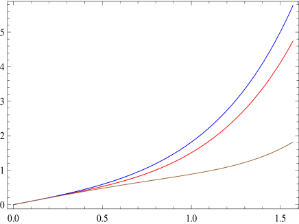
Figure 1: Graphs of $f_{i}(t)$; the lowest one (brown) is $f_{1}(t)$ while the highest one (blue) is $f_{2}(t)$, and the middle one (red) is $f_{3}(t)$.

Correspondingly, the model surfaces for the geodesic ball $B(q,r_{0})$ in the above three cases can be chosen to be $M^{-}_{i}:=[0,r_{0})\times_{f_{i}(t)}\mathbb{S}^{n-1}$ ($i=1,2,3$). Since $K^{2}_{lower}(t)\leq K^{3}_{lower}(t)\leq K^{1}_{lower}(t)$ for $0\leq t<r_{0}$, then by the Sturm-Picone comparison theorem, we know that $f_{2}(t)\leq f_{3}(t)\leq f_{1}(t)$ for $0\leq t<r_{0}$ (see also Figure 1). As we have pointed out in Section 2, if the Gaussian curvature is nonnegative around $q\in\mathcal{T}$, then the model surface could be locally embedded into a surface of revolution in $\mathbb{R}^{3}$. So, here we could only get a picture for $M_{1}^{-}$ by using Mathematica. One can see Figure 2 in [9] (equivalently, Figure 2.3 in [18]) for the graph of $M_{1}^{-}$. When $f^{\prime}(t)$ starts to be greater than $1$ for some $t=t_{0}$, the model surface stops being isometrically embeddedable in $\mathbb{R}^{3}$, which implies that its picture can not be drawn when $t\geq t_{0}$. We call this $t_{0}$ “stopping time”. The “stopping time” $t_{0}$ for our model surface $M_{1}^{-}$ here is $t_{0}\approx 1.097$ (cf. example 6.1 in [9] or example 2.5.1 in [18]). For more information about the properties of the model manifolds of prescribed manifolds, one could see [9, 18] in detail.

Without loss of generality, we can choose $\alpha=\pi/2$ in Case (III). Denote the upper bounds of the first Dirichlet eigenvalue of the $p$-Laplacian in the above three cases by JM1, JM2 and JM3, respectively. Then, for different $p$ and $\delta$, we have the Table 1 below.

Table 1 makes sense, since it is difficult to compute the first Dirichlet eigenvalue of the $p$-Laplacian on a geodesic ball of $\mathcal{T}$, but, this table supplies us a range for the first eigenvalue.

For Case (I) and Case (III), the lower bounds of the Gaussian curvature w.r.t. the base point $q\in\mathcal{T}$ are given by continuous functions of the distance parameter $t$, which are not constant functions. By (1) of Remark 3.3, we know that if we apply Theorem 3.2, then the corresponding estimates for the first eigenvalue of the $p$-Laplacian will be sharper than the estimates obtained by using theorem 1.1 in [19] or theorem 3 in [22]. Of course, one may also use other examples about elliptic paraboloid and saddle shown in [9] to show the advantage of our Theorem 3.2, but, this example about torus is enough.

In addition, for given $n$, $p$ and $R$, estimates (4.4) give an interval where the first Dirichlet eigenvalue of the $p$-Laplacian on the ball $B(R)\subseteq\mathbb{R}^{n}$ locates. Although, in [3], the authors there have shown that one can get the approximate value of the first eigenvalue of the $p$-Laplacian of the ball $B(R)$ in the Euclidean space via the inverse power method, we still think (4.4) is useful, since it can be used to check the validity of this approximate value of the first eigenvalue at the first glance.

Table 1  Numerical values of the upper bounds of the first Dirichlet eigenvalue of the $p$-Laplacian $\delta=\frac{\pi}{24}$ $\delta=\frac{\pi}{12}$ $\delta=\frac{\pi}{6}$ $\delta=\frac{\pi}{4}$ $\delta=\frac{\pi}{3}$ $\delta=\frac{5\pi}{12}$ $p=1.1$ 27.1285 12.5875 5.76216 3.615235 2.63716 2.18278 $p=1.5$ 129.804 45.6551 15.8426 8.43068 5.41996 3.98597 JM1 $p=2$ 633.49 157.585 38.6834 16.7921 9.29658 6.02468 $p=2.5$ 2643.65 465.081 80.7606 28.6185 13.6868 7.87571 $p=2.9$ 7788.71 1038.53 136.711 41.1932 17.5401 9.19918 $p=1.1$ 27.3318 12.9637 6.43987 4.52941 3.69959 3.27638 $p=1.5$ 130.731 46.9574 17.6385 10.5314 7.67446 6.24665 JM2 $p=2$ 637.815 161.89 42.9072 20.8735 13.1648 9.60296 $p=2.5$ 2661.1 477.379 89.3207 35.4141 19.3209 12.609 $p=2.9$ 7839.06 1065.42 150.92 50.8147 24.6856 14.7308 $p=1.1$ 27.1916 12.7303 6.13046 4.27308 3.53423 3.17492 $p=1.5$ 130.086 46.1295 16.7496 9.8136 7.1877 5.93221 JM3 $p=2$ 634.785 159.108 40.7077 19.3037 12.1299 8.9332 $p=2.5$ 2648.82 469.358 84.735 32.6294 17.6292 11.5564 $p=2.9$ 7803.57 1047.8 143.195 46.7425 22.4114 13.3865

5 Some facts about the heat eqaution

If we want to get the existence, or even give an explicit expression, of the solution for the heat equation (1.4) with a prescribed initial condition or (Dirichlet or Neumann) boundary condition, we need to use a tool named heat kernel.

Definition 5.1.

A fundamental solution, which is called the heat kernel, of the heat equation on a prescribed Riemannian manifold $M$ is a continuous function $H(x,y,t)$, defined on $M\times{M}\times(0,\infty)$, which is $C^{2}$ with respect to $x$, $C^{1}$ with respect to $t$, and which satisfies

$$L_{x}p=0,\qquad\lim\limits_{t\rightarrow 0}H(x,y,t)=\delta_{y}(x),$$

where $\delta_{y}(x)$ is the Dirac delta function, that is, for all bounded continuous function $f$ on $M$, we have, for every $y\in{M}$,

$$\lim\limits_{t\rightarrow 0}\int_{M}H(x,y,t)f(x)dV(x)=f(y).$$

By constructing a parametrix, the existence of the heat kernel on compact or complete Riemannian manifolds, or even manifolds with boundaries subject to either Dirichelt or Neumann boundary conditions can be obtained (see, for instance, [4]). In fact, for a complete Riemannian manifold, one can have the following.

Theorem 5.2.

([23]) Let $M$ be a complete Riemannian manifold, then there exists a heat kernel $H(x,y,t)\in{C^{\infty}(M\times{M}\times\mathbb{R}^{+})}$ such that (I) $H(x,y,t)=H(y,x,t)$, (II) $\lim\limits_{t\rightarrow 0}H(x,y,t)=\delta_{x}(y)$, (III) $\left(\Delta-\frac{d}{dt}\right)H=0$, (IV) $H(x,y,t)=\int_{M}H(x,z,t-s)H(z,y,s)dV(z)$.

In the next section, we would like to focus on the heat kernels of geodesic balls on complete manifolds, and successfully obtain a comparison result, which can be seen as an extension of Debiard-Gaveau-Mazet’s comparison result in [7] and Cheeger-Yau’s comparison result in [6], for the heat kernel with a Dirichlet or Neumann boundary condition – see Theorem 6.6 for the precise statement. There is a connection between the heat kernel and the eigenvalues of the Laplace operator. One can get a glance about this relation from the following conclusion (cf. [4], p. 169).

Theorem 5.3.

(The Sturm-Liouville decomposition for the Dirichlet eigenvalue problem) Given a normal domain $\Omega$ in a Riemannian manifold $M$, there exists a complete orthonormal basis $\{\phi_{1},\phi_{2},\phi_{3},\cdots\}$ of $L^{2}(\Omega)$ consisting of Dirichlet eigenfunctions of the Laplacian $\Delta$, with $\phi_{j}$ having eigenvalue $\lambda_{j}$ satisfying

$$0<\lambda_{1}<\lambda_{2}\leq\lambda_{3}\leq\cdots\uparrow\infty.$$

In particular, each eigenvalue has finite multiplicity, and

$$\phi_{j}\in{C^{\infty}(\Omega)\cap\bar{C}^{1}(\Omega)},$$

where $\bar{C}^{1}(\Omega)$ is the set of functions $v$ satisfying that $v$ is $C^{1}$ on $\Omega$, and can be extended to a continuous function on $\overline{\Omega}$, and moreover, the gradient ${\rm{grad}}{v}$ can be extended to a continuous vector field on $\overline{\Omega}$.

Finally, the heat kernel $H(x,y,t)$ on $\Omega$ satisfies

$$H(x,y,t)=\sum\limits_{j=1}^{\infty}e^{-\lambda_{j}t}\phi_{j}(x)\phi_{j}(y),$$

with convergence absolute, and uniform, for each $t>0$. In particular,

$$\int_{\Omega}H(x,x,t)dV(x)=\sum\limits_{j=1}^{\infty}e^{-\lambda_{j}t}.$$

By using Theorem 5.3 and the comparison result for the heat kernel, Theorem 6.6, we can supply another ways to prove the most part of theorems 3.3 and 4.4 in [9] – see Theorem 6.8 for the precise statement.

6 Estimates for the heat kernel

As before, for a complete $n$-dimensional Riemannian manifold $M$, denote by $B(p,r_{0})$ the open geodesic ball with center $p$ and radius $r_{0}$ of $M$. Let $V_{n}(p^{-},r_{0})$ be the geodesic ball with center $p^{-}$ and radius $r_{0}$ of an $n$-dimensional spherically symmetric manifold $M^{-}=[0,l)\times_{f}\mathbb{S}^{n-1}$ with respect to $p^{-}$, and let $V_{n}(p^{+},r_{0})$ be the geodesic ball with center $p^{+}$ and radius $r_{0}$ of an $n$-dimensional spherically symmetric manifold $M^{+}=[0,l)\times_{f}\mathbb{S}^{n-1}$ with respect to $p^{+}$, where the model spaces $M^{+}$ and $M^{-}$ can be determined by the upper and lower bounds of the radial sectional and Ricci curvatures w.r.t. the given point $p\in{M}$. This fact has been shown in the previous sections. Denote by $H(p,y,t)$ the heat kernel on $M$, and by $H_{+}(p^{+},q,t)$ and $H_{-}(p^{-},q,t)$ the heat kernels on $M^{+}$ and $M^{-}$, respectively. In this section, we would like to give an upper and lower bound for the heat kernel. However, before that, we need to use the following facts in [6].

First, we need the following concept, which is used to describe model spaces considered in [6].

Definition 6.1.

An $n$-dimensional manifold $\mathscr{M}^{n}$ is an open model, if the following conditions hold:

(I) For some $x\in\mathscr{M}^{n}$ and $0<R\leq\infty$, $\mathscr{M}^{n}=B(x,R)$ (the open ball of radius $R$ about $x$) and $\exp_{x}|B_{0}(R)$, with $B_{0}(R)\subseteq{T_{x}}\mathscr{M}^{n}$, is a diffeomorphism.

(II) For all $r<R$, the mean curvature of the distance sphere $S(x,r)$ is constant on $S(x,r)$. Moreover, a model $\mathscr{M}^{n}$ is an open Ricci model if its metric, when written in polar coordinates, is of the form

$$dr^{2}+f^{2}(r)h,$$

where $h$ is the standard metric on $\mathbb{S}^{n-1}$. A compact Riemannian manifold $\mathscr{M}^{n}$ is a closed model (resp., closed Ricci model) if, for some $x$, $\mathscr{M}=\overline{B(x,R)}$ and $B(x,R)$ is an open model (resp., Ricci model).

Clearly, by Definition 2.1, we know that a spherically symmetric manifold must be an open or closed Ricci model with respect to its base point.

We also need the following lemma which shows us the positivity of the heat kernel.

Lemma 6.2.

([6]) Let $\Omega$ be a domain in a Riemannian manifold. Then for either Dirichlet or Neumann boundary conditions, the heat kernel $H(x,y,t)$ on $\Omega$ satisfies $H(x,y,t)>0$ for $t>0$.

By proposition 2.2 and lemma 2.3 of [6], we have the following lemma.

Lemma 6.3.

([6]) (I) Let $\mathscr{M}^{n}$ be an $n$-dimensional open model (with Dirichlet or Neumann boundary conditions) or a closed model. Then its heat kernel $H(x,y,t)=H(d(x,y),t)$ depends only on variables $r:=d(x,y)$ and $t$, with $d$ the distance function on $\mathscr{M}^{n}$.

(II) Conversely, let $\mathscr{M}^{n}=B(x,R)$ or $\overline{B(x,R)}$, and assume that $\overline{B(x,R)}$ is complete. Then if the heat kernel $H(x,y,t)$ depends only on on variables $r:=d(x,y)$ and $t$, it follows that $\mathscr{M}^{n}$ is a model.

(III) Let $\mathscr{M}^{n}$ be a model, and let $H(r,t)$ be the fundamental solution of the heat equation (with respect to Dirichlet or Neumann boundary conditions if $\mathscr{M}^{n}$ is open). Then, for all $r,t>0$, we have

$$\frac{\partial}{\partial{r}}H(r,t)<0.$$

By Lemma 6.3, we have the following.

Corollary 6.4.

For the model space $M^{+}$ (resp., $M^{-}$), its heat kernel $H_{+}(p^{+},y,t)=H_{+}(r_{1},t)$ (resp., $H_{-}(p^{-},y,t)=H_{-}(r_{2},t)$) depends only on variables $r_{1}:=d_{M^{+}}(p^{+},y)$ (resp., $r_{2}:=d_{M^{-}}(p^{-},y)$) and $t$, where $d_{M^{+}}$ (resp., $d_{M^{-}}$) denotes the distance function on $M^{+}$ (resp., $M^{-}$). Moreover, for all $t>0$, we have

$$\frac{\partial}{\partial{r_{1}}}H_{+}(r_{1},t)<0,\qquad\left({\rm{resp.,}}~{}\frac{\partial}{\partial{r_{2}}}H_{-}(r_{2},t)<0\right).$$

We also need the following strong maximum (resp., minimum) principle (cf. [4], p. 180).

Theorem 6.5.

Given a Riemannian manifold $M$ with the Laplacian $\Delta$, and the associated heat operator $L=\Delta-\frac{\partial}{\partial{t}}$. Let $u(x,t)$ be a bounded continuous function on $M\times[0,T]$, which is $C^{2}$ with respect to the variable $x\in{M}$, and $C^{1}$ with respect to $t\in[0,T]$, and which satisfies

$$Lu\geq 0\qquad\left(Lu\leq 0\right)$$

on $M\times(0,T)$. If there exists $(x_{0},t_{0})$ in $M\times(0,T]$ such that

$$u(x_{0},t_{0})=\sup\limits_{M\times[0,T]}u(x,t),\qquad\left({\rm{resp.,}}~{}u(x_{0},t_{0})=\inf\limits_{M\times[0,T]}u(x,t)\right),$$

then

$$u|M\times[0,t_{0}]=u(x_{0},t_{0}).$$

Clearly, the heat equation satisfies both the strong maximum principle and the strong minimum principle, which implies that the solution of the heat equation can only achieve its maximum or minimum on the boundary $\overline{M\times(0,T]}-M\times(0,T]$. One can easily get a proof of Theorem 6.5 in [8] when $M$ is diffeomorphic to a domain in Euclidean space. By a standard continuation argument, then one is able to get a proof for an arbitrary manifold $M$.

By applying Theorems 2.6 and 2.7, Corollary 6.4 and Theorem 6.5, we can prove the following.

Theorem 6.6.

If $M$ is a complete n-dimensional Riemannian manifold with a radial sectional curvature upper bound $k(t)=-\frac{f^{\prime\prime}(t)}{f(t)}$ w.r.t. a point $p\in{M}$, then, for $r_{0}<\min\{inj(p),l\}$, we have

$$H(p,y,t)\geq{H_{+}(d_{M^{+}}(p^{+},q),t)}$$ (6.1)

holds for all $(y,t)\in{B(p,r_{0})\times(0,\infty)}$ with $d_{M^{+}}(p^{+},q)=d_{M}(p,y)$ for any $q\in{M^{+}}$, where $d_{M^{+}}$ and $d_{M}$ denote the distance functions on $M^{+}$ and $M$, respectively. The equality in (6.1) holds at some $(y_{0},t_{0})\in{B(p,r_{0})\times(0,\infty)}$ if and only if $B(p,r_{0})$ is isometric to $V_{n}(p^{+},r_{0})$.

On the other hand, if $M$ is a complete $n$-dimensional Riemannian manifold with a radial Ricci curvature lower bound $(n-1)k(t)=-\frac{(n-1)f^{\prime\prime}(t)}{f(t)}$ w.r.t. a point $p\in{M}$, then, for all $(y,t)\in{B(p,r_{0})\times(0,\infty)}$ and $r_{0}<\min\{l(p),l\}$ with $l(p)$ defined as in (2.4), we have

$$H(p,y,t)\leq{H_{-}(d_{M^{-}}(p^{-},q),t)}$$ (6.2)

with $d_{M^{-}}(p^{-},q)=d_{M}(p,y)$ for any $q\in{M^{-}}$, where $d_{M^{-}}$ and $d_{M}$ denote the distance functions on $M^{-}$ and $M$, respectively. The equality in (6.2) holds at some $(y_{0},t_{0})\in{B(p,r_{0})\times(0,\infty)}$ if and only if $B(p,r_{0})$ is isometric to $V_{n}(p^{+},r_{0})$. (The boundary condition will either be Dirichlet or Neumann.)

Proof.

By the assumptions on curvatures in Theorem 6.6, we know that the model space $M^{+}=[0,l)\times_{f}\mathbb{S}^{n-1}$ or $M^{-}=[0,l)\times_{f}\mathbb{S}^{n-1}$ is determined by solving the initial value problem

$$\left\{\begin{array}[]{lll}f^{\prime\prime}(t)+k(t)f(t)=0,\\ f(0)=0,\\ f^{\prime}(0)=1.&\end{array}\right.$$

Now, assume that the radial sectional curvature of $M$ is bounded from above by a continuous function $k(t)=-f^{\prime\prime}(t)/f(t)$ w.r.t. $p\in{M}$. By applying Theorem 5.2, we have

$$H(p,y,t)-H_{+}(d_{M^{+}}(p^{+},q),t)=H(p,y,t)-H_{+}(d_{M}(p,y),t)$$

$$= H(p,y,t)-H_{+}(r_{1}(p,y),t)$$

$$= \int_{0}^{t}\int_{B(p,r_{0})}\frac{d}{ds}\left[H_{+}(r_{1}(p,z),t-s)H(z,y,s)\right]dV(z)ds$$

$$= -\int_{0}^{t}\int_{B(p,r_{0})}\frac{\partial}{\partial{s}}\left[H_{+}(r_{1}(p,z),t-s)\right]H(z,y,s)dV(z)ds$$

$$+\int_{0}^{t}\int_{B(p,r_{0})}H_{+}(r_{1}(p,z),t-s)\frac{\partial{H}}{\partial{s}}(z,y,s)dV(z)ds$$

$$= -\int_{0}^{t}\int_{B(p,r_{0})}\Delta_{M^{+}}H_{+}(r_{1}(p,z),t-s)H(z,y,s)dV(z)ds$$

$$+\int_{0}^{t}\int_{B(p,r_{0})}H_{+}(r_{1}(p,z),t-s)\Delta_{M}H(z,y,s)dV(z)ds,$$

where $\Delta_{M^{+}}$, $\Delta_{M}$ are the Laplace operators on $M^{+}$ and $M$, respectively. Since $r_{0}<\min\{inj(p),l\}$, by applying Green’s formula, and using either Dirichlet or Neumann boundary condition, we have

$$\int_{B(p,r_{0})}H_{+}(r_{1}(p,y),t)\cdot\Delta_{M}H=\int_{B(p,r_{0})}\Delta_{M}H_{+}(r_{1}(p,y),t)\cdot{H}.$$

So, we obtain

$$H(p,y,t)-H_{+}(d_{M^{+}}(p^{+},q),t)=\int_{0}^{t}\int_{B(p,r_{0})}\big{[}\Delta_{M}H_{+}(r_{1},t-s)-\Delta_{M^{+}}H_{+}(r_{1}(p,y),$$

$$\qquad\qquad t-s)\big{]}\cdot H(z,y,s)dV(z)dt.$$ (6.4)

On the other hand, in the geodesic spherical coordinates near $p$ or $p^{+}$, for function of $r_{1}(p,y)=d_{M^{+}}(p^{+},q)=d_{M}(p,y)$, we have

$$\Delta_{M^{+}}=\frac{\partial^{2}}{\partial{r_{1}^{2}}}+\frac{\left[f^{n-1}(r_{1})\right]^{\prime}}{f^{n-1}(r_{1})}\frac{\partial}{\partial{r_{1}}},$$

$$\Delta_{M}=\frac{\partial^{2}}{\partial{r_{1}}^{2}}+\frac{\left[det\mathbb{A}(r_{1},\xi)\right]^{\prime}}{det\mathbb{A}(r_{1},\xi)}\frac{\partial}{\partial{r_{1}}}=\frac{\partial^{2}}{\partial{r_{1}}^{2}}+\frac{\left(\sqrt{|g|}\right)^{\prime}}{\sqrt{|g|}}\frac{\partial}{\partial{r_{1}}},$$

where $\mathbb{A}(r_{1},\xi)$ is the path of linear transformations defined in Section 2, and $\sqrt{|g|}$ is defined as (2.2). So, by Theorem 2.7, we have

$$\Delta_{M}H_{+}(r_{1},t-s)-\Delta_{M^{+}}H_{+}(r_{1}(p,z),t-s)=\left[\frac{\left(\sqrt{|g|}\right)^{\prime}}{\sqrt{|g|}}-\frac{\left[f^{n-1}(r_{1})\right]^{\prime}}{f^{n-1}(r_{1})}\right]\frac{\partial{H_{+}}}{\partial{r_{1}}}\geq 0.\quad$$ (6.5)

Substituting (6.5) into (6), together with Lemma 6.2, we obtain

$$H(p,y,t)-H_{+}(d_{M^{+}}(p^{+},q),t)\geq 0,$$

which implies (6.1). When equality in (6.1) holds at some $(y_{0},t_{0})\in{B(p,r_{0})\times(0,\infty)}$, by Theorem 6.5, we know that $H(p,y,t)={H_{+}(d_{M^{+}}(p^{+},q),t)}=H(p,y_{0},t_{0})$ on $B(p,r_{0})\times[0,t_{0}]$. Together with (6.5), we know that

$$\frac{\left(\sqrt{|g|}\right)^{\prime}}{\sqrt{|g|}}=\frac{\left[f^{n-1}(r_{1})\right]^{\prime}}{f^{n-1}(r_{1})}$$

holds on $B(p,r_{0})$. Then by Theorem 2.7, we have

$$\mathbb{A}(r_{1},\xi)=f(r_{1})I$$

for all $r_{1}\leq{r_{0}}$, which implies that $B(p,r_{0})$ is isometric to $V_{n}(p^{+},r_{0})$.

Now, assume that the radial Ricci curvature of $M$ is bounded from below by a continuous function $(n-1)k(t)=-(n-1)f^{\prime\prime}(t)/f(t)$ w.r.t. $p\in{M}$, and $r_{0}<\min\{l(p),l\}$. Since the geodesic ball $B(p,r_{0})$ maybe has points on the cut-locus, which leads to the invalidity of the path of linear transformations $\mathbb{A}$, we need to use a limit procedure shown in [6] to avoid this problem. As the previous case, by applying Theorem 5.2, we have

$$H(p,y,t)-H_{-}(d_{M^{-}}(p^{-},q),t)=H(p,y,t)-H_{-}(d_{M}(p,y),t)$$ (6.6)

$$= H(p,y,t)-H_{-}(r_{2}(p,y),t)$$

$$= -\int_{0}^{t}\int_{B(p,r_{0})}\frac{\partial}{\partial{s}}\left[H_{-}(r_{2}(p,z),t-s)\right]H(z,y,s)dV(z)ds$$

$$+\int_{0}^{t}\int_{B(p,r_{0})}H_{-}(r_{2}(p,z),t-s)\frac{\partial{H}}{\partial{s}}(z,y,s)dV(z)ds.$$

For any $\xi\in{S^{n-1}_{p}}\subseteq{T_{p}M}$, let $g(\xi):=\min\{d_{\xi},r_{0}\}$ with $d_{\xi}$ defined in Section 2. Clearly, $g(\xi)$ is a continuous function on the unit sphere $S^{n-1}_{p}$. As in [5], one can choose a sequence of smooth functions $g_{\epsilon}$ on $S^{n-1}_{p}$, with $g_{\epsilon}(\xi)<g(\xi)$ for any $\xi\in{S^{n-1}_{p}}$, such that $g_{\epsilon}$ converges uniformly to $g$ as $\epsilon\rightarrow 0$ and the set

$$V_{\epsilon}=\{\exp_{p}(t\xi)|t\leq{g_{\epsilon}(\xi)}\}$$

is compact. Clearly, $V_{\epsilon}$ is within the cut locus of $p$. So, the expression (6.6) becomes

$$H(p,y,t)-H_{-}(d_{M^{-}}(p^{-},q),t)=H(p,y,t)-H_{-}(r_{2}(p,y),t)$$

$$= \lim\limits_{\epsilon\rightarrow 0}\Big{\{}-\int_{0}^{t}\int_{V_{\epsilon}}\frac{\partial}{\partial{s}}\left[H_{-}(r_{2}(p,z),t-s)\right]H(z,y,s)dV(z)ds$$

$$+\int_{0}^{t}\int_{V_{\epsilon}}H_{-}(r_{2}(p,z),t-s)\frac{\partial{H}}{\partial{s}}(z,y,s)dV(z)ds\Big{\}}$$

$$= \lim\limits_{\epsilon\rightarrow 0}\Big{\{}-\int_{0}^{t}\int_{V_{\epsilon}}\Delta_{M^{-}}\left[H_{-}(r_{2}(p,z),t-s)\right]H(z,y,s)dV(z)ds$$

$$+\int_{0}^{t}\int_{V_{\epsilon}}H_{-}(r_{2}(p,z),t-s)\Delta_{M}H(z,y,s)dV(z)ds\Big{\}},$$

where $\Delta_{M^{-}}$, $\Delta_{M}$ are the Laplace operators on $M^{-}$ and $M$, respectively. Then, similar to the previous case, by applying Theorem 2.6 and Corollary 6.4, we can obtain

$$H(p,y,t)-H_{1}(d_{M^{-}}(p^{-},y),t)$$ (6.7)

$$= \lim\limits_{\epsilon\rightarrow 0}\left\{\int_{0}^{t}\int_{V_{\epsilon}}\left[\Delta_{M}H_{-}(r_{2},t-s)-\Delta_{M^{-}}H_{-}(r_{2}(p,z),t-s)\right]h(z,y,s)dV(z)dt\right\}$$

$$= \lim\limits_{\epsilon\rightarrow 0}\left\{\int_{0}^{t}\int_{V_{\epsilon}}\left[\frac{\left[J^{n-1}(r_{2},\xi)\right]^{\prime}}{J^{n-1}(r_{2},\xi)}-\frac{\left[f^{n-1}(r_{2})\right]^{\prime}}{f^{n-1}(r_{2})}\right]\frac{\partial{H_{-}}}{\partial{r_{2}}}H(z,y,s)dV(z)dt\right\}\leq 0,$$

with the function $J(r_{2},\xi)$ defined as (2.2), which implies (6.2). When equality in (6.2) holds at some $(y_{0},t_{0})\in{B(p,r_{0})\times(0,\infty)}$, by Theorem 6.5, we know that $H(p,y,t)={H_{-}(d_{M^{-}}(p^{-},q),t)}=H(p,y_{0},t_{0})$ on $B(p,r_{0})\times[0,t_{0}]$. Together with (6.7), we know that

$$\frac{\left[J^{n-1}(r_{2},\xi)\right]^{\prime}}{J^{n-1}(r_{2},\xi)}=\frac{\left[f^{n-1}(r_{2})\right]^{\prime}}{f^{n-1}(r_{2})}$$

holds on $B(p,r_{0})$. Then by Theorem 2.6, we have

$$\mathbb{A}(r_{2},\xi)=f(r_{2})I$$

for all $r_{2}\leq{r_{0}}$, which implies that $B(p,r_{0})$ is isometric to $V_{n}(p^{-},r_{0})$. Our proof is finished. ∎

Remark 6.7.

In fact, the completeness of the prescribed manifold $M$ is a little strong to get the comparison results (6.1) and (6.2) for the heat kernel. In [6], Cheeger and Yau have shown that if the injectivity radius at some point $p$ of a prescribed manifold $M$ is bounded from below, then, under the assumptions on curvature therein, a lower bound can be given for the heat kernel of geodesic balls on $M$. However, here we prefer to assume that the prescribed manifold $M$ is complete, since if $M$ is complete, then for $B(p,r_{0})\subseteq{M}$ with $r_{0}$ finite we can always find optimally continuous bounds for the radial Ricci and sectional curvatures w.r.t. $p$ (see (2.14) and (2.15)). This implies that the assumption on the completeness of $M$ is feasible.

Theorem 5.3 shows us a connection between the Dirichlet heat kernel and the Dirichlet eigenvalue of the Laplacian. Here we would like to use this connection to give another ways to prove the following Cheng-type eigenvalue inequalities for the Laplace operator, which have been given in [9].

Theorem 6.8.

If $M$ is a complete n-dimensional Riemannian manifold with a radial Ricci curvature lower bound $(n-1)k(t)=-\frac{(n-1)f^{\prime\prime}(t)}{f(t)}$ w.r.t. a point $p\in{M}$, then, $r_{0}<\min\{l(p),l\}$ with $l(p)$ defined as in (2.4), we have

$$\lambda_{1}(B(p,r_{0}))\leq\lambda_{1}\left(V_{n}(p^{-},r_{0})\right).$$ (6.8)

On the other hand, if $M$ is a complete $n$-dimensional Riemannian manifold with a radial sectional curvature upper bound $k(t)=-\frac{f^{\prime\prime}(t)}{f(t)}$ w.r.t. a point $p\in{M}$, then, for $r_{0}<\min\{inj(p),l\}$, we have

$$\lambda_{1}\left(B(p,r_{0})\right)\geq\lambda_{1}\left(V_{n}(p^{+},r_{0})\right).$$ (6.9)

Here $\lambda_{1}(\cdot)$ in (6.8) and (6.9) denotes the first eigenvalue of the corresponding geodesic ball.

Proof.

Here we would like to use a method similar to that of theorem 1 in p. 104-105 of [23]. As before, denote separately the Dirichlet heat kernels of $B(p,r_{0})$, $V_{n}(p^{-},r_{0})$ by $H(p,y,t)$ and $H_{-}(d_{M^{-}}(p^{-},q),t)$, with $r_{2}(p,y)=d_{M}(p,y)=d_{M^{-}}(p^{-},q)$, where $d_{M}$ and $d_{M^{-}}$ are distance functions on $M$ and $M^{-}$, respectively. If $M$ has a radial Ricci curvature lower bound $(n-1)k(t)=-(n-1)f^{\prime\prime}(t)/f(t)$ w.r.t. $p\in{M}$, and $r_{0}<\min\{l(p),l\}$, then by Theorem 6.6, we have

$$H(p,p,t)\geq{H_{-}(0,t)=H_{-}(r_{2}(p,p),t)}$$ (6.10)

for all $t>0$. Furthermore, by Theorem 5.3, we can obtain

$$H(p,p,t)=\sum\limits_{i=1}^{\infty}e^{-\lambda_{i}t}\phi_{i}^{2}(p),$$

$$H_{-}(0,t)=\sum\limits_{i=1}^{\infty}e^{-\tilde{\lambda}_{i}t}\tilde{\phi}_{i}^{2}(0),$$

with $\lambda_{i}=\lambda_{i}\left(B(p,r_{0})\right)$, $\tilde{\lambda}_{i}=\lambda_{i}\left(V_{n}(p^{-},r_{0})\right)$, and $\phi_{i}$, $\tilde{\phi}_{i}$ the corresponding eigenfunctions. Together with (6.10), it follows that

$$e^{-\lambda_{1}t}\left[\phi^{2}_{1}(p)+e^{-(\lambda_{2}-\lambda_{1})t}\phi^{2}_{2}(p)+\cdots\right]\geq e^{-\tilde{\lambda}_{1}t}\left[\tilde{\phi}^{2}_{1}(0)+e^{-(\tilde{\lambda}_{2}-\tilde{\lambda}_{1})t}\tilde{\phi}^{2}_{2}(0)+\cdots\right],$$

which is equivalent with

$$\phi^{2}_{1}(p)+e^{-(\lambda_{2}-\lambda_{1})t}\phi^{2}_{2}(p)+\cdots\geq e^{(\lambda_{1}-\tilde{\lambda}_{1})t}\left[\tilde{\phi}^{2}_{1}(0)+e^{-(\tilde{\lambda}_{2}-\tilde{\lambda}_{1})t}\tilde{\phi}^{2}_{2}(0)+\cdots\right].$$ (6.11)

Since $\phi^{2}_{1}(p)>0$, $\tilde{\phi}^{2}_{1}(0)>0$, and $\lambda_{m}>\lambda_{1}$ (resp., $\tilde{\lambda}_{m}>\tilde{\lambda}_{1}$) for any $m\geq 2$, letting $t\rightarrow\infty$ in (6.11) results in

$$\lambda_{1}-\tilde{\lambda}_{1}\leq 0,$$

which implies

$$\lambda_{1}\left(B(p,r_{0})\right)\leq\lambda_{1}\left(V_{n}(p^{-},r_{0})\right).$$

On the other hand, by applying Theorem 6.6 and a similar method as above, we can easily obtain that for $r_{0}<\min\{inj(p),l\}$, the inequality

$$\lambda_{1}\left(B(p,r_{0})\right)\geq\lambda_{1}\left(V_{n}(p^{+},r_{0})\right)$$

holds when $M$ has a radial sectional curvature upper bound $k(t)=-f^{\prime\prime}(t)/f(t)$ w.r.t. $p$. Our proof is finished. ∎

Remark 6.9.

In the above proof of Theorem 6.8, when $\lambda_{1}\left(B(p,r_{0})\right)=\lambda_{1}\left(V_{n}(p^{-},r_{0})\right)$, we cannot get the characterization, $B(p,r_{0})$ is isometric to $V_{n}(p^{-},r_{0})$, for this equality as theorem 3.3 in [9]. In fact, if $\lambda_{1}\left(B(p,r_{0})\right)=\lambda_{1}\left(V_{n}(p^{-},r_{0})\right)$ here, we can only obtain that $\lim_{t\rightarrow\infty}H(p,p,t)=\lim_{t\rightarrow\infty}H_{-}(0,t)$. We are not sure whether there exists some $t_{0}<\infty$ such that $H(p,p,t_{0})=H_{-}(0,t_{0})$ or not, which leads to the fact that we cannot use the characterization for the equality of (6.2) in Theorem 6.6. This can be seen as the limitation of this new way. The same situation happens to the equality $\lambda_{1}\left(B(p,r_{0})\right)=\lambda_{1}\left(V_{n}(p^{+},r_{0})\right)$.

References

• [1] C.S. Barroso, G.P. Bessa, Lower bounds for the first Laplacian eigenvalue of geodesic balls of spherically symmetric manifolds, Int. J. Appl. Math. Stat. 6 (2006) 82–86.
• [2] M. Belloni, B. Kawohl, A direct uniqueness proof for equations involving the $p$-Laplace operator, Manuscripta Math. 109 (2002) 229–231.
• [3] R. J. Biezuner, G. Ercole and E.M. Martins, Computing the first eigenvalue of the $p$-Laplacian via the inverse power method, J. Funct. Anal. 257 (2009) 243–270.
• [4] I. Chavel, Eigenvalues in Riemannian geometry, Academic Press, New York, 1984.
• [5] J. Cheeger and D. Gromoll, The splitting theorem for manifolds of non-negative Ricci curvature, J. Differ. Geom. 6 (1971) 119–128.
• [6] J. Cheeger and S. T. Yau, A lower bound for the heat kernel, Commun. Pure Appl. Math. 34 (1981) 465–480.
• [7] A. Debiard, B. Gaveau, and E. Mazet, ThΓ©or$\grave{e}$m de comparisons en gΓ©omΓ©trie riemanniene, Publ. R.I.M.S., Kyoto Univ. 12 (1976) 391–425.
• [8] L. C. Evance, Partial Differential Equation, American Mathematical Society, 1998.
• [9] P. Freitas, J. Mao and I. Salavessa, Spherical symmetrization and the first eigenvalue of geodesic disks on manifolds, submitted (2012).
• [10] M.P. Gaffney, A special Stokes’s theorem for complete Riemannian manifolds, Ann. of Math. 60 (1) (1954) 140–145.
• [11] M.P. Gaffney, The heat equation method of Milgram and Rosenbloom for open Riemannian manifolds, Ann. of Math. 60 (3) (1954) 458–466.
• [12] A.Β Gray, Tubes, Addison-Wesley, New York, 1990.
• [13] A. Grigor’yan, Isoperimetric inequalities and capacities on Riemannian manifolds, Operator Theory, Advances and Applications, vol. 110, The Maz’ya Anniversary Collection, vol. 1, Birkh$\ddot{\rm{a}}$user, Basel, 1999, pp.139-153.
• [14] N. N. Katz and K. Kondo, Generalized space forms, Trans. Amer. Math. Soc. 354 (2002) 2279-2284.
• [15] B. Kawohl and V. Fridman, Isoperimetric estimates for the first eigenvalue of the $p$-Laplace operator and the Cheeger constant, Comment. Math. Univ. Carolin. 44 (4) (2003) 659–667.
• [16] L. Lefton and D, Wei, Numerical approximation of the first eigenpair of the $p$-Laplacian using finte elements and the penalty method, Numer. Funct. Anal. Optim. 18 (1997) 389–399.
• [17] J. Mao, A class of rotationally symmetric quantum layers of dimension 4, J. Math. Anal. Appl. 397 (2) (2013) 791–799.
• [18] J.Β Mao, Eigenvalue estimation and some results on finite topological type, Ph.D.Β thesis, IST-UTL, 2013.
• [19] A.-M. Matei, First eigenvalue for the $p$-Laplace operator, Nonlinear Anal. TMA 39 (8) (2000) 1051–1068.
• [20] B. O’Neill, Semi-Riemannian Geometry with applications to relativity, vol. 103 of Pure and Applied mathematics, Academic Press, San Diego, 1983.
• [21] P.Β Petersen, Riemannian Geometry, Second Edition, vol.171 of Graduate Texts in Mathematics, Springer, New York, 2006.
• [22] H. Takeuchi, On the first eigenvalue of the $p$-Laplacian in a Riemannian manifold, Tokyo J. Math. 21 (1998) 135–140.
• [23] R. Schoen and S. T. Yau, Lectures on Differential Geometry, International Press, Boston, 1994.