Probing Color Octet Electrons at the LHC

Abstract

Models with quark and lepton compositeness predict the existence of colored partners of the Standard Model leptons. In this paper we study the LHC phenomenology of a charged colored lepton partner, namely the color octet electron, $e_{8}$ in an effective theory framework. We explore various mechanisms for resonant production of $e_{8}$’s. With the pair production channel the 14 TeV LHC can probe $e_{8}$’s with masses up to 2.5 TeV (2.8 TeV) with 100 fb^-1 (300 fb^-1) of integrated luminosity. A common feature in all the resonant production channels is the presence of two high $p_{T}$ electrons and at least one high $p_{T}$ jet in the final state. Using this feature, we implement a search method where the signal is a combination of pair and single production events. This method has potential to increase the LHC reach significantly. Using the combined signal we estimate the LHC discovery potential for the $e_{8}$’s. Our analysis shows that the LHC with 14 TeV center-of-mass energy and 100 fb^-1 (300 fb^-1) of integrated luminosity can probe $e_{8}$’s with masses up to 3.4 TeV (4 TeV) for the compositeness scale of 5 TeV.

I Introduction

All the experimental outcomes so far indicate that the Standard Model (SM) is the correct effective theory of elementary particles for energies below the TeV scale. If the recently discovered Higgs-like boson at the Large Hadron Collider (LHC) at CERN is confirmed to be the SM Higgs, it will complete the experimental verification of the particle spectrum of the SM HiggsAtlas ; HiggsCMS . However, despite its spectacular success with the experiments, there remain some issues like the hierarchy problems, fermion family replication etc. that are not properly addressed in the SM. Many theoretical attempts have been made to resolve these issues. Beyond-the-SM (BSM) alternatives like supersymmetry, extra dimensions and quark-lepton compositeness are some well-known examples. Many of the BSM theories predict the existence of new particles with masses near the TeV scale. Two detectors of the LHC, namely ATLAS and CMS, are presently looking for the signatures of some of these new particles.

Of the various BSM scenarios, the quark-lepton composite models assume that the SM particles may not be fundamental and just as the proton has constituent quarks, they are actually bound states of substructural constituents (preons) Pati:1974yy . These constituents are visible only beyond a certain energy scale known as the compositeness scale. A typical consequence of quark-lepton compositeness is the appearance of colored particles with nonzero lepton numbers (leptogluons, leptoquarks) and excited leptons etc. Some composite models naturally predict the existence of leptogluons ($l_{8}$) Pati:1974yy ; Terazawa:1976xx ; Neeman:1979wp ; Harari:1979gi ; Shupe:1979fv ; Fritzsch:1981zh ; D'Souza:1992tg that are color octet fermions with nonzero lepton numbers. Several studies on the collider searches of leptoquarks and excited fermions can be found in the literature Chatrchyan:2012dn ; Chatrchyan:2012sv ; ATLAS:2012af but there are only a few similar studies on $l_{8}$’s. Various signatures of color octet leptons at different colliders were investigated in some earlier papers Rizzo:1985dn ; Rizzo:1985ud ; Streng:1986my ; Celikel:1998tm ; Hewett:1997ce ; Celikel:1998dj . Recently some important production processes of the $l_{8}$ have been analyzed for future colliders like the Large Hadron-electron Collider (LHeC), the International Linear Collider (ILC) and the Compact Linear Collider (CLiC) Sahin:2010dd ; Akay:2010sw . We briefly review the limits on (charged) color octet leptons available in the literature. The lower mass limit of color octet charged leptons quoted in the latest Particle Data Book Beringer:2012pdg is only 86 GeV. This limit is from the 23-years-old Tevatron data Abe:1989es from the pair production channel. A mass limit of $M_{l_{8}}>\mathcal{O}(110)$ GeV from the direct pair production via color interactions has been derived from $p\bar{p}$ collider data in Baur:1985ud . Lower limits on the leptogluons masses were derived by the JADE collaboration from the $t$-channel contribution to the total hadronic cross section, $M_{l_{8}}\gtrsim(240~{}\textrm{GeV})^{3}/4\Lambda^{2}$ (where $\Lambda$ is the compositeness scale) and from direct production via one photon exchange, $M_{l_{8}}\gtrsim 20$ GeV Bartel:1987zp . In Ref. Abt:1993nr , the compositeness scale $\Lambda\lesssim 1.8$ TeV was excluded at 95$\%$ confidence level (CL) for $M_{l_{8}}\simeq 100$ GeV and $\Lambda\lesssim 200$ GeV for $M_{l_{8}}\simeq 200$ GeV. It is also mentioned in Hewett:1997ce that the D0 cross section bounds on $eejj$ events exclude leptogluons with masses up to 200 GeV and could naively place the constraint $M_{l_{8}}\gtrsim 325$ GeV.

In this paper we study the LHC discovery potential for a generic color octet partner of a charged lepton, namely the color octet electron, $e_{8}$. Although, in this paper, we consider only color octet electrons, our results are applicable for the color octet partner of the muon, i.e., $\mu_{8}$ also. The paper is organized as follows: in Sec. II we display the interaction Lagrangian and decay width of $e_{8}$. In Sec. III we discuss various $e_{8}$ production processes at the LHC. In Sec. IV we discuss the LHC reach for $e_{8}$’s. Finally, in Sec. V we summarize and offer our conclusions.

II The Lagrangian

Assuming lepton flavor conservation we consider a general Lagrangian for the color octet electrons including terms allowed by the gauge symmetries of the SM,

$$\mathcal{L}=\bar{e}_{8}^{a}i\gamma^{\mu}\left(\partial_{\mu}\delta^{ac}+g_{s}f^{abc}G^{b}_{\mu}\right)e_{8}^{c}-M_{e_{8}}\bar{e}_{8}^{a}e_{8}^{a}+\mathcal{L}_{int}.$$ (1)

For simplicity, we have ignored the terms with electroweak couplings. The interaction part $(\mathcal{L}_{int})$ contains all the higher dimensional operators. In this paper we consider only the following dimension five terms that contain the interaction between ordinary electrons and color octet ones Beringer:2012pdg ,

$$\mathcal{L}_{int}=\frac{g_{s}}{2\Lambda}G^{a}_{\mu\nu}\left[\bar{e}_{8}^{a}\sigma^{\mu\nu}\left(\eta_{L}e_{L}+\eta_{R}e_{R}\right)\right]+H.c.\,.$$ (2)

Here $G^{a}_{\mu\nu}$ is the gluon field strength tensor, $\Lambda$ is the scale below which this effective theory is valid and $\eta_{L/R}$ are the chirality factors. Since, electron chirality conservation implies $\eta_{L}\eta_{R}=0$, we set $\eta_{L}=1$ and $\eta_{R}=0$ in our analysis.

From the interaction Lagrangian given in Eq. 2 we see that an $e_{8}$ can decay to a gluon and an electron (two-body decay mode), i.e., $e_{8}\to eg$ or two gluons and an electron (three-body decay mode), i.e., $e_{8}\to egg$ (via the $e_{8}egg$ vertex). However, compared to the $e_{8}eg$ decay rate, the three-body decay rate is suppressed by an extra power of $\alpha_{s}$ and phase space suppression. If one includes dimension six or higher dimensional terms in the Lagrangian then, in general, $e_{8}$ can have other many-body decay modes like, e.g., $e_{8}\to eqq$ via a four fermion $e_{8}eqq$ vertex. However, these many-body decays will be much more suppressed than the two-body decay. Hence, in this paper, we focus only on the dominant two-body decay mode. With $\eta_{L}=1$ and $\eta_{R}=0$, the decay width of $e_{8}$ can be written as,

$$\Gamma_{e_{8}}=\frac{\alpha_{s}(M_{e_{8}})M_{e_{8}}^{3}}{4\Lambda^{2}}.$$ (3)

III Production at the LHC

In this section we discuss various production mechanisms of $e_{8}$’s at the LHC and present the production cross sections for different channels. To obtain the cross sections, we have first implemented the Lagrangian of Eq. 1 in FeynRules version 1.6.0 Christensen:2008py to generate Universal FeynRules Output (UFO) Degrande:2011ua format model files suitable for MadGraph5 Alwall:2011uj that we have used to estimate the cross sections. We have used CTEQ6L1 Parton Distribution Functions (PDFs) Pumplin:2002vw for all our numerical computations.

At a hadron collider like the LHC, resonant productions of $e_{8}$’s can occur via $gg$, $gq$ and $qq$ initiated processes where $q$ can be either a light quark or a bottom quark. The gluon PDF dominates at the low $x$ region whereas the quark PDFs take over at the high $x$ region. Thus, depending on $M_{e_{8}}$, all of the $gg$, $gq$ and $qq$ initiated processes can contribute significantly to the production of $e_{8}$’s at the LHC.

For the resonant production $e_{8}$’s at colliders, two separate channels are generally considered in the literature – one is the pair production Hewett:1997ce ; Celikel:1998dj and the other is the single production of $e_{8}$ Rizzo:1985dn ; Rizzo:1985ud ; Streng:1986my ; Celikel:1998tm ; Sahin:2010dd . In general, pair production of a colored particle is considered mostly model independent. This is because the universal strong coupling constant $g_{S}$ controls the dominant pair production processes unlike the single production processes where the cross section depends more on various model parameters like couplings and scales etc. However, as we shall see, for $e_{8}$’s, the $t$-channel electron exchange diagrams can contribute significantly to the pair production making it more model dependent.

III.1 Pair Production (${\bf gg,qq\to e_{8}e_{8}}$)

(a)		(b)		(c)		(d)

(a)

Figure 1: Parton level Feynman diagrams for $pp\to e_{8}e_{8}$ processes at the LHC.

At the LHC, pair production of $e_{8}$’s is $gg$ or $qq$ initiated – see Fig. 1 where we have shown the parton level Feynman diagrams for this channel. Of these, only the electron exchange diagram, shown in Fig 1d, contains the $\Lambda$ dependent $gee_{8}$ vertex. In Fig. 2 we show the $pp\to e_{8}e_{8}$ cross section as a function of $M_{e_{8}}$ for two different choices of $\Lambda$, $\Lambda=M_{e_{8}}$ and $\Lambda=5$ TeV, at the 14 TeV LHC. In Fig. 3 we have plotted $\delta\sigma$ as a function of $\Lambda$ to show the dependence of the pair production cross section on $\Lambda$ for $M_{e_{8}}=1$ and 2 TeV, where $\delta\sigma$ is a measure of the contribution of the electron exchange diagram and is defined as,

$$\delta\sigma(\Lambda)=\sigma(\Lambda)-\sigma(\Lambda\rightarrow\infty).$$ (4)

As $\Lambda$ increases the contribution coming from the electron exchange diagrams decreases and for $\Lambda\gg M_{e_{8}}$ becomes negligible. So the pair production is model independent only for very large $\Lambda$.

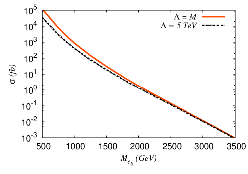
(a)

Figure 2: The cross sections for $pp\to e_{8}e_{8}$ as a function of $M_{e_{8}}$ for $\Lambda=M_{e_{8}}$ and $\Lambda=5$ TeV at the 14 TeV LHC.

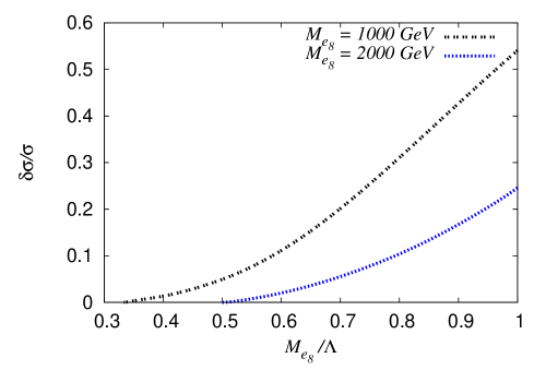
(a)

Figure 3: Dependence of $\delta\sigma/\sigma$ (defined in Eq. 4) on $M_{e_{8}}/\Lambda$ for $M_{e_{8}}=1$ TeV and 2 TeV at the 14 TeV LHC.

After being produced as pairs at the LHC, each $e_{8}$ decays into an electron (or a positron) and a gluon at the parton level, i.e.,

$$gg/qq\to e_{8}e_{8}\to eejj.$$

For large $M_{e_{8}}$, these two jets and the lepton pair will have high $p_{T}$. This feature can be used to isolate the $e_{8}$ pair production events from the SM backgrounds at the LHC.

III.2 Two-body Single Production (${\bf gg,qq\to e_{8}e}$)

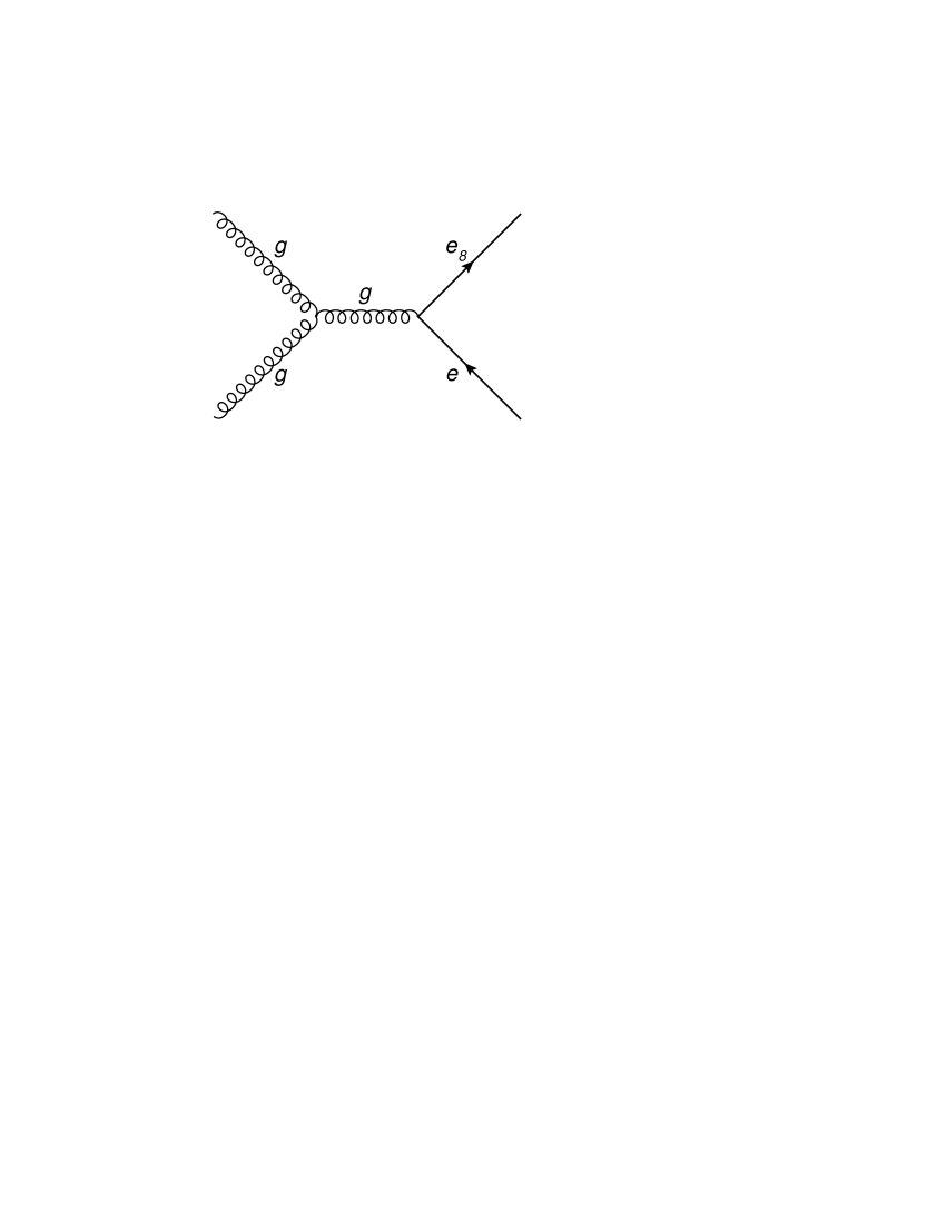
(a)		(b)		(c)		(d)

(a)

Figure 4: Parton level Feynman diagrams for $pp\to e_{8}e$ processes at the LHC.

The two-body single production channel where an $e_{8}$ is produced in association with an electron can have either $gg$ or $qq$ initial states as shown in Fig. 4. This channel is model dependent as each Feynman diagram for the $pp\to e_{8}e$ process contains a $\Lambda$ dependent vertex. In Fig. 5 we show the $pp\to e_{8}e$ cross sections as a function of $M_{e_{8}}$ with $\Lambda=M_{e_{8}}$ and 5 TeV and 10 TeV at the 14 TeV LHC.

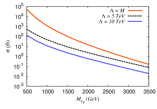
(a)

Figure 5: The cross sections for $pp\to e_{8}e$ as a function of $M_{e_{8}}$ for $\Lambda=M_{e_{8}}$, 5 TeV and 10 TeV at the 14 TeV LHC.

As the $e_{8}$ decays, this process gives rise to an $eej$ final state at the parton level. The $e$ and the $j$ produced from the decay of the $e_{8}$, have high $p_{T}$. The other $e$ also possesses very high $p_{T}$ as it balances against the massive $e_{8}$.

III.3 Three-body Single Production (${\bf gg,gq,qq\to e_{8}ej}$)

Apart from the pair and the two-body single productions, we also consider single production of an $e_{8}$ in association with an electron and a jet. The $pp\to e_{8}ej$ process includes three different types of diagrams as follows:

1. The diagrams where the $ej$ pair is coming from another $e_{8}$. Though there are three particles in the final state, this type of diagram effectively corresponds to two-body pair production process.

2. The two-body single production ($pp\to e_{8}e$) process with a jet radiated from the initial state (ISR) or final state (FSR) or intermediate virtual particles can lead to an $e_{8}ej$ final state.

3. A new set of diagrams that are different from the two types of diagrams mentioned above. These new channels can proceed through $gg$, $qq$ and $gq$ initial states as shown in Fig. 6.

(a)		(b)		(c)		(d)
(e)		(f)		(g)		(h)
(i)		(j)		(k)		(l)

(a)

Figure 6: Parton level Feynman diagrams for $pp\to e_{8}ej$ processes of the third type at the LHC.

This new set of diagrams has not been considered so far in the literature. It is difficult to compute the total contribution of these diagrams in a straight forward manner with a leading order parton level matrix element calculation because of the presence of soft radiation jet emission diagrams. In order to get an estimation of the contribution of these new diagrams without getting into the complicacy of evaluating the soft jet emission diagrams, here, in this section, we present the cross section only for the $gq$ initiated processes, i.e. $gq\to e_{8}ej$ since the first and the second types of diagrams can not be initiated by $gq$ state. In Fig. 7 we show the cross section of the $gq\to e_{8}ej$ process along with the $pp\to e_{8}e_{8}$ and the $pp\to e_{8}e$ processes. We find that the cross sections even for the $gq$ initiated subset can be comparable to the $pp\to e_{8}e_{8}/e_{8}e$ processes for large $M_{e_{8}}$ despite the facts that these new diagrams have three-body final states and are suppressed by one extra power of the coupling (either $g_{S}$ or $g_{S}/\Lambda$) compared to the two-body single and pair production processes. However, since there is one less $e_{8}$ compared to the pair production process, depending on the coupling the three-body phase space of the single production can be comparable or even larger to the two-body phase space of the pair production for large $M_{e_{8}}$.

After the $e_{8}$ decay, the three-body single production process is characterized by an $eejj$ final state like the pair production. However, unlike the pair production, here one of the jets can have a low transverse momentum.

III.4 Indirect Production (${\bf gg\to ee}$)

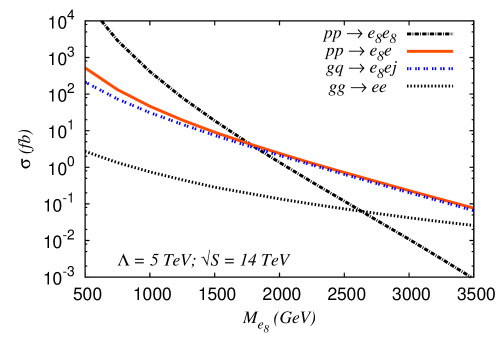
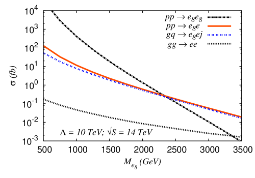
(a)		(b)

(a)

Figure 7: Cross sections for $pp\to e_{8}e_{8}$, $pp\to e_{8}e$, $gq\to e_{8}ej$ and $gg\xrightarrow{e_{8}}ee$ processes for $\Lambda=5$ TeV and 10 TeV at the 14 TeV LHC. The $\sigma(gq\to e_{8}ej)$ is computed with the following kinematical cuts: $p_{T}(j)>25$ GeV and $|y(j)|<2.5$.

(a)

Figure 8: Parton level Feynman diagram for indirect production of $e_{8}$’s at the LHC.

So far we have considered only resonant production of $e_{8}$’s. However, a t-channel exchange of the $e_{8}$ can convert a gluon pair to an electron-positron pair at the LHC (Fig. 8). Similar indirect productions in the context of future linear colliders such as the ILC and CLiC have been analyzed in Akay:2010sw . Indirect production is less significant because the amplitude is proportional to $1/\Lambda^{2}$. Moreover, at the LHC this is also color suppressed because of the color singlet nature of the final states. In Fig. 7 we also show the cross section of the indirect production process at the LHC.

IV LHC Discovery Potential

From Fig. 7 we see that for small $M_{e_{8}}$, the pair production cross section is larger than the other channels. As $M_{e_{8}}$ increases, it decreases rapidly due to phase-space suppression and the single production channels (both the two-body and the three-body) take over the pair production (the crossover point depends on $\Lambda$). Hence, if $\Lambda$ is not too high, the single production channels will have better reach than the pair production channel and so, to estimate the LHC discovery reach, we consider both the pair and the single production channels. However, while estimating for the single production channels we have to remember that because of the radiation jets, it will be difficult to separate the two-body and the three-body single productions at the LHC. So, in this paper, we consider a selection criterion that combines events from all the production processes at the LHC.

IV.1 Combined Signal

To design the selection criterion mentioned above we first note some of the characteristics of the final states of the resonant production processes ,

1. Process $pp\to e_{8}e_{8}\to(eg)(eg)$ has two high $p_{T}$ electrons and two high $p_{T}$ jets in the final state.

2. Process $pp\to e_{8}e\to(eg)e$ has two high $p_{T}$ electrons and one high $p_{T}$ jet in the final state.

3. Process $pp\to e_{8}ej\to(eg)ej$ has two high $p_{T}$ electrons and at least one high $p_{T}$ jet in the final state.

All these processes have one common feature that they have two high $p_{T}$ electrons and a high $p_{T}$ jet in the final state. Hence if we demand that the signal events should have two high $p_{T}$ electrons and at least one high $p_{T}$ jet, we can capture events from all the above mentioned production processes. To estimate the number of signal events that pass the above selection criterion we combine the events from all the production channels mentioned in the previous section. However, as already pointed out, it is difficult to estimate the number of signal events with only a matrix element (ME) level Monte Carlo computation due to the presence of soft radiation jets. Hence we use the MadGraph ME generator to compute the hard part of the amplitude and Pythia6 (via the MadGraph5-Pythia6 interface) for parton showering. We also match the matrix element partons with the parton showers to estimate the inclusive signal without double counting (see the Appendix A for more details on the matched signal).

IV.2 SM Backgrounds

With the selection criterion mentioned above, the SM backgrounds are characterized by the presence of two opposite sign electrons and at least one jet in the final state. At the LHC, the main source of $e^{+}e^{-}$ pairs (with high $p_{T}$) is the $Z$ decay . Hence we compute the inclusive $Z$ production as the main background. Here, too, we compute this by matching the matrix element partons of $Z+n$ jets ($n=0,1,2,3$) processes with the parton showers using the shower-$k_{T}$ scheme Alwall:2008qv . For the background, we also consider some potentially significant processes to produce $e^{+}e^{-}$ pairs,

$$pp\to tt\to(bW)(bW)\to(be\nu_{e})(be\nu_{e}),$$

$$pp\to tW\to bWW\to(be\nu_{e})(e\nu_{e}),$$

$$pp\to WW\to(e\nu_{e})(e\nu_{e}).$$

Note that all these processes have missing energy because of the $\nu_{e}$’s in the final state. In Table 1 we show the relative contributions of these backgrounds generated with some basic kinematical cuts (to be described shortly) on the final states . As mentioned, we see in Table 1 that the inclusive $Z$ contribution overwhelms the other background processes.

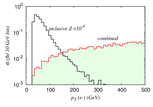
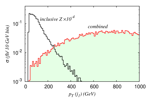
(a)		(b)
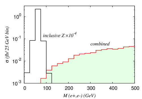
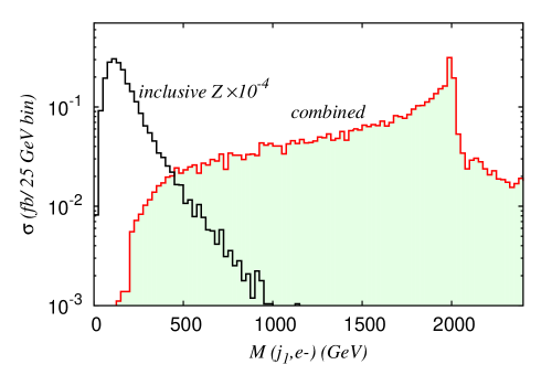
(c)		(d)

(a)

Figure 9: Comparison between various distributions for the combined signal with $M_{e_{8}}=2$ TeV ($\Lambda=5$ TeV) and the inclusive $Z$ background for the 14 TeV LHC. The inclusive $Z$ background is shown after multiplying by a factor of $10^{-4}$. For each plot we indicate the corresponding bin size in the Y-axis label.

Process		Cross section (fb)
$Z+nj$		$2.11E4$
$tt$		$1.95E3$
$tW$		132.15
$WW$		7.51
Total		$2.32E4$

Table 1: The main SM backgrounds to the combined production of $e_{8}$’s obtained after applying the Basic cuts (see text for definition).

IV.3 Kinematical Cuts

In Fig. 9a we display the $p_{T}$ distributions of $e$’s from the combined signal and the inclusive $Z$ production, respectively. For the signal, we have chosen $M_{e_{8}}=2$ TeV and $\Lambda=5$ TeV. As expected, the distribution for the $e$ coming from the background has a peak at about $M_{Z}/2$ but there is no such peak for the signal. We can also see the difference between the $p_{T}$ distributions of the leading $p_{T}$ jets for the signal and the background in Fig. 9b. We also display the distributions of $M(e^{+},e^{-})$ (see Fig.9c) and $M(e^{-},j_{1})$ (see Fig. 9d) (where $j_{1}$ denotes the leading $p_{T}$ jet) which show very different natures for the signal and the background.

Motivated by these distributions, we construct some kinematical cuts to separate the signal from the background:

1. Basic cuts
   For $x,y=e^{+},e^{-},j_{1},j_{2}$ ($j_{1}$ and $j_{2}$ denote the first two of the $p_{T}$ ordered jets respectively),

   1. $p_{T}(x)>25$ GeV

   2. Rapidity, $|\eta(x)|<2.5$

   3. Radial distance, $\Delta R(x,y)_{x\neq y}\geq 0.4$

2. Discovery cuts

   1. All the Basic cuts

   2. $p_{T}(e^{+}/e^{-})>150$ GeV; $p_{T}(j_{1})>100$ GeV

   3. $M(e^{+},e^{-})>150$ GeV

   4. For at least one combination of $(e,j_{i})$: $|M(e,j_{i})-M_{e_{8}}|\leq 0.2M_{e_{8}}$ where $e=e^{+}$ or $e^{-}$ and $j_{i}=j_{1}$ or $j_{2}$.

The cut on $M(e^{+},e^{-})$ can remove the $Z$ inclusive background almost completely. For our estimation of the LHC discovery reach we also use the cut on $M(e,j_{i})$ to demand that either of the electrons reconstruct to an $e_{8}$ when combined with any one of $j_{1}$ or $j_{2}$. Although this cut involves an unknown parameter, namely $M_{e_{8}}$, it can be implemented in the actual experiment by performing a scan of $M_{e_{8}}$ over a range (say, 0.5 TeV to 4 TeV). While scanning, for each value of $M_{e_{8}}$, one can apply this cut on all the events. If $e_{8}$ exists within the scanned region, it will lead to an excess of events (compared to the SM) around the actual value of $M_{e_{8}}$. We find that the Discovery cuts can reduce the SM background drastically. Especially for higher $M_{e_{8}}$ the background becomes much smaller compared to the signal, making it essentially background free. In Table 2 we show the signal with the above two cuts applied.

$M_{e_{8}}$	$\Lambda=5$ TeV		$\Lambda=10$ TeV
(GeV)	Basic (fb)	Disco. (fb)	Basic (fb)	Disco. (fb)
500	2.73E4	1.31E4	2.70E4	1.27E4
750	2.63E3	1.93E3	2.59E3	1.91E3
1000	442.95	367.20	415.35	347.16
1250	105.21	90.25	91.99	80.45
1500	31.73	27.25	24.54	21.86
1750	11.53	9.76	7.52	6.71
2000	4.77	3.92	2.59	2.28
2250	2.26	1.80	0.99	0.85
2500	1.18	0.91	0.42	0.36
2750	0.65	0.49	0.20	0.16
3000	0.37	0.27	0.11	0.08
3250	0.22	0.16	0.06	0.04
3500	0.13	0.09	0.03	0.02

Table 2: The combined signal after basic and Discovery cuts (see text for the definitions of the cuts) for $\Lambda=5$ TeV and 10 TeV for different $M_{e_{8}}$.

IV.4 LHC Reach with Combined Signal

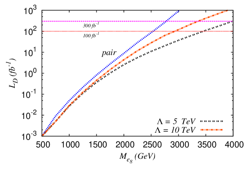
(a)

Figure 10: The required luminosity for discovery ($L_{D}$) as a function of $M_{e_{8}}$ with $\Lambda=5$ TeV and 10 TeV at the 14 TeV LHC for combined production with Discovery cuts (see text for the definitions of the cuts). The $L_{D}$ for pair production is computed after demanding two $e_{8}$’s are reconstructed instead of one.

We define the luminosity requirement for the discovery of color octet electrons at the LHC as following:

$$L_{D} = Max(L_{5},L_{10})$$ (5)

where $L_{5}$ denotes the luminosity required to attain $5\sigma$ statistical significance for $S/\sqrt{B}$ and $L_{10}$ is the luminosity required to observe 10 signal events. We show $L_{D}$ as a function of $M_{e_{8}}$ for the Discovery cuts in Fig. 10 for $\Lambda=5$ TeV and 10 TeV at the 14 TeV LHC. In Fig. 10 we also plot the $L_{D}$ using only the pair production process. To estimate the pair production from the combined signal we apply a set of kinematical cuts almost identical to the Discovery cuts except that now we demand that the two electrons and the two leading $p_{T}$ jets reconstruct to two $e_{8}$’s instead of one:

1. Pair production extraction cuts

   1. All the Basic cuts

   2. $p_{T}(e^{+}/e^{-})>150$ GeV; $p_{T}(j_{1})>100$ GeV

   3. $M(e^{+},e^{-})>150$ GeV

   4. $|M(e^{+},j_{k})-M_{e_{8}}|\leq 0.2M_{e_{8}}$ and $|M(e^{-},j_{l})-M_{e_{8}}|\leq 0.2M_{e_{8}}$ with $k\neq l=\{1,2\}$.

In Fig. 10, $L_{D}$ goes as $L_{10}$ for both pair and combined productions, as in these cases the backgrounds become quite small compared to the signals. With the Discovery cuts the reach goes up to 3.4 TeV and 2.9 TeV (4 TeV and 3.3 TeV) with 100 fb^-1 (300 fb^-1) integrated luminosity for $\Lambda=5$ TeV and 10 TeV respectively at the 14 TeV LHC. This also shows that for $\Lambda=5$ TeV (10 TeV) with combined signal at 14 TeV LHC with 300 fb^-1 integrated luminosity the reach goes up from the pair production by almost 1.2 TeV (0.5 TeV). However, we should keep in mind that this increase depends on $\Lambda$. As the single production cross section goes like $1/\Lambda^{2}$, if $\Lambda$ is smaller than 5 TeV then the reach of the combined production will increase even more but for higher $\Lambda$ (like $\Lambda=10$ TeV as shown in Fig. 10) its $L_{D}$ plot will approach more towards the pair production plot.

V Summary and Conclusions

In this paper we have studied the phenomenology of $e_{8}$’s at the LHC and estimated the discovery potential of such particles at the LHC. We have explored various production channels of $e_{8}$’s at the LHC namely, the pair, the two-body single, the three-body single and the indirect production channels. The contribution of the three-body single production channel is comparable to that of the two-body single production channel. While the pair production cross section dominates the other channels for low $M_{e_{8}}$, for high values of $M_{e_{8}}$ the single productions become significant. The 14 TeV LHC with 100 fb^-1 (300 fb^-1) of integrated luminosity can probe $e_{8}$’s with masses up to 2.5 TeV (2.8 TeV) with only pair production. We have demonstrated how this reach can be increased further by combining signal events from different production processes. However, this increment is $\Lambda$ dependent as the single production cross section scales as $1/\Lambda^{2}$. For $\Lambda=5$ TeV (10 TeV) the increment is about 0.9 TeV (0.4 TeV) with 100 fb^-1 of integrated luminosity at the 14 TeV LHC and with 300 fb^-1 of integrated luminosity it is about 1.2 TeV (0.5 TeV).

We point out that our analysis can also be used to probe $\Lambda$, the compositeness scale, for any fixed $M_{e_{8}}$. This is possible because of the scaling of the single production cross section with $\Lambda$. For example, for $M_{e_{8}}=2$ TeV and $\Lambda=10$ TeV we estimate the single production cross section as $1.2$ fb which we obtain from the events that pass the Discovery cuts but not the Pair production extraction cuts. By computing $L_{10}$ (i.e., the luminosity requirement to observe 10 signal events) from this we can conclude that for $M_{e_{8}}=2$ TeV the 14 TeV LHC with 100 fb^-1 (300 fb^-1) of integrated luminosity can probe $\Lambda\sim 35$ TeV ($55$ TeV). This can be useful as the present searches of leptoquarks at the LHC generally focus on their pair production which is mostly independent of $\Lambda$. However, even with the single production of leptoquarks at the LHC it is difficult to probe the compositeness scale directly. This can be seen in an effective theory picture as, unlike leptogluon, the interaction Lagrangian of leptoquarks with the SM particles is dominated by renormalizable dimension four operators.

We note that the data from the current leptoquark searches at the LHC can be used to search for $e_{8}$’s also. The current data for leptoquarks Chatrchyan:2012dn ; Chatrchyan:2012sv already puts some constraints on the masses of the $l_{8}$’s. For example the data from the search for 1^st generation charged leptoquark in the pair production channel clearly rules out a color octet electron of mass less than 900 GeV (see Fig. 10 of Chatrchyan:2012dn ), since the pair production cross section of color octet electrons is always larger than the pair production cross section of color triplet leptoquarks of the same mass due to color enhancement .

Appendix A Preparation of Matched Signal

For the signal, we match the matrix element partons with the parton showers using the shower-$k_{T}$ scheme Alwall:2008qv in MadGraph5 with the matching scale $Q_{cut}\sim 50$ GeV. We generate the combined signal including the different production processes as discussed in section IV,

$$pp \xrightarrow{e_{8}} ee\textrm{ (includes $P_{ind}$)}$$

$$pp \xrightarrow{e_{8}} ee+1\textrm{-j (includes $P_{ind}+$ 1-j, $P_{2Bs}$ )}$$

$$pp \xrightarrow{e_{8}} ee+2\textrm{-j (includes $P_{ind}+$ 2-j, $P_{2Bs}+$ 1-j, $P_{pair}$ , $P_{3Bs}^{3}$ )}$$

$$pp \xrightarrow{e_{8}} ee+3\textrm{-j (includes $P_{ind}+$ 3-j, $P_{2Bs}+$ 2-j, $P_{pair}+$ 1-j, $P_{3Bs}^{3}+$ 1-j)}$$ (6)

where $P_{pair}$, $P_{2Bs}$, $P_{3Bs}^{3}$ and $P_{ind}$ are the pair, two-body single, three-body single of the third type and indirect productions respectively. We refer the reader to Alwall:2008qv and the references therein for more details on the matching scheme and the procedure.

References

- (1) G. Aad et al. [ATLAS Collaboration], Phys. Lett. B 716, 1 (2012) [arXiv:1207.7214 [hep-ex]].
- (2) S. Chatrchyan et al. [CMS Collaboration], Phys. Lett. B 716, 30 (2012) [arXiv:1207.7235 [hep-ex]].
- (3) J. C. Pati and A. Salam, Phys. Rev. D 10, 275 (1974) [Erratum-ibid. D 11, 703 (1975)].
- (4) H. Terazawa, K. Akama and Y. Chikashige, Phys. Rev. D 15, 480 (1977).
- (5) Y. Ne’eman, Phys. Lett. B 81, 190 (1979).
- (6) H. Harari, Phys. Lett. B 86, 83 (1979).
- (7) M. A. Shupe, Phys. Lett. B 86, 87 (1979).
- (8) H. Fritzsch and G. Mandelbaum, Phys. Lett. B 102, 319 (1981).
- (9) I. A. D’Souza and C. S. Kalman, Singapore, Singapore: World Scientific (1992) 108 p
- (10) S. Chatrchyan et al. [CMS Collaboration], Phys. Rev. D 86, 052013 (2012) [arXiv:1207.5406 [hep-ex]].
- (11) S. Chatrchyan et al. [CMS Collaboration], arXiv:1210.5629 [hep-ex].
- (12) G. Aad et al. [ATLAS Collaboration], Phys. Rev. D 85, 072003 (2012) [arXiv:1201.3293 [hep-ex]].
- (13) T. G. Rizzo, Phys. Rev. D 33, 1852 (1986).
- (14) T. G. Rizzo, Phys. Rev. D 34, 133 (1986).
- (15) K. H. Streng, Z. Phys. C 33, 247 (1986).
- (16) A. Celikel and M. Kantar, Turk. J. Phys. 22, 401 (1998).
- (17) J. L. Hewett and T. G. Rizzo, Phys. Rev. D 56, 5709 (1997) [hep-ph/9703337].
- (18) A. Celikel, M. Kantar and S. Sultansoy, Phys. Lett. B 443, 359 (1998).
- (19) M. Sahin, S. Sultansoy and S. Turkoz, Phys. Lett. B 689, 172 (2010) [arXiv:1001.4505 [hep-ph]].
- (20) A. N. Akay, H. Karadeniz, M. Sahin and S. Sultansoy, Europhys. Lett. 95, 31001 (2011) [arXiv:1012.0189 [hep-ph]].
- (21) J. Beringer et al. [Particle Data Group], Phys. Rev. D 86, 010001 (2012).
- (22) F. Abe et al. [CDF Collaboration], Phys. Rev. Lett. 63, 1447 (1989).
- (23) U. Baur and K. H. Streng, Phys. Lett. B 162, 387 (1985).
- (24) W. Bartel et al., Z Phys. C 36, 15 (1987).
- (25) I. Abt et al. [H1 Collaboration], Nucl. Phys. B 396, 3 (1993).
- (26) N. D. Christensen and C. Duhr, Comput. Phys. Commun. 180, 1614 (2009) [arXiv:0806.4194 [hep-ph]].
- (27) C. Degrande, C. Duhr, B. Fuks, D. Grellscheid, O. Mattelaer and T. Reiter, Comput. Phys. Commun. 183, 1201 (2012) [arXiv:1108.2040 [hep-ph]].
- (28) J. Alwall, M. Herquet, F. Maltoni, O. Mattelaer and T. Stelzer, JHEP 1106, 128 (2011) [arXiv:1106.0522 [hep-ph]].
- (29) J. Pumplin, D. R. Stump, J. Huston, H. L. Lai, P. M. Nadolsky and W. K. Tung, JHEP 0207, 012 (2002) [hep-ph/0201195].
- (30) J. Alwall, S. de Visscher and F. Maltoni, JHEP 0902, 017 (2009) [arXiv:0810.5350 [hep-ph]].
- (31) D. Goncalves-Netto, D. Lopez-Val, K. Mawatari, I. Wigmore and T. Plehn, arXiv:1303.0845 [hep-ph].