Limiting distributions of continuous-time random walks with superheavy-tailed waiting times

Abstract

We study the long-time behavior of the scaled walker (particle) position associated with decoupled continuous-time random walk which is characterized by superheavy-tailed distribution of waiting times and asymmetric heavy-tailed distribution of jump lengths. Both the scaling function and the corresponding limiting probability density are determined for all admissible values of tail indexes describing the jump distribution. To analytically investigate the limiting density function, we derive a number of different representations of this function and, by this way, establish its main properties. We also develop an efficient numerical method for computing the limiting probability density and compare our analytical and numerical results.

I INTRODUCTION

The continuous-time random walks (CTRWs), i.e., cumulative jump processes which are characterized by a joint probability density of waiting time and jump length, play a significant role in many areas of science. The reason is that a large variety of physical, biological and other systems are often modeled by two random variables that can be interpreted as the waiting time between successive transitions (jumps) of the system into new states and the transition measure (jump length). For example, the CTRW model and its modifications can be used to describe anomalous diffusion and transport in disordered media SM ; MK ; AH ; KRS , human mobility BHG ; SKWB , financial SGM ; MMW ; Scal ; MNPW and seismic HS ; PAG data.

According to the theory of CTRWs MW (see also Refs. MK ; AH ), the probability density $P(x,t)$ of the particle position $X(t)$ depends only on the joint probability density of waiting time and jump length. Unfortunately, even in the simplest (decoupled) case when the joint density is a product of waiting-time density $p(\tau)$ and jump-length density $w(\xi)$, the representation of $P(x,t)$ in terms of special functions is known in a few cases KZ ; Bar ; GPSS . In contrast, the long-time behavior of $P(x,t)$ that determines the diffusion and transport properties of walking particles is studied analytically in much more detail Tun ; SKW ; WWH ; Kot ; MS . Specifically, the asymptotic behavior of the scaled particle position $Y(t)=a(t)X(t)$ is investigated in Ref. Kot . In this work, the scaling function $a(t)$ and the distribution function of $Y(t)$ at $t\to\infty$ are obtained for all waiting-time and jump densities characterized by finite second moments or heavy tails.

A special case of CTRWs with superheavy-tailed distributions of waiting time was first considered in HW . Because all fractional moments of these distributions are infinite, they can be used to model extremely anomalous behavior of systems and processes as, e.g., iterated maps DrKl , ultraslow kinetics CKS , superslow diffusion DK1 , and Langevin dynamics DKH ; DK2 . For the CTRWs characterized by arbitrary superheavy-tailed distributions of waiting time, the scaling function $a(t)$ and the corresponding limiting probability density $\mathcal{P}(y)$ of $Y(\infty)$ have already been found for the jump densities having finite second moments DK3 and symmetric heavy tails DYBKL . In the present work, we report a comprehensive theoretical and numerical studies of the long-time behavior of the reference CTRWs in the general case of asymmetric jump densities characterized by heavy tails.

The paper is organized as follows. In Sec. II, we describe the CTRW model, formulate the problem of the limiting probability density and list some previously obtained results. In Sec. III, we find the scaling function $a(t)$ and the limiting probability density $\mathcal{P}(y)$ in terms of the inverse Fourier transform for all possible cases. A number of alternative representations of the limiting density and its main properties are obtained in Sec. IV. Here, we derive $\mathcal{P}(y)$ in terms of (i) the inverse Mellin transform, (ii) the Laplace transform, (iii) the Fox $H$ function, and (iiii) the series expansion. Using the series and Laplace representations of the limiting probability density, in Sec. V we determine its short- and long-distance behavior. In Sec. VI, we develop a method for the numerical evaluation of $\mathcal{P}(y)$ and compare the analytical and numerical results. Our findings are summarized in Sec. VII. Finally, a short derivation of the fractional equation for $\mathcal{P}(y)$ is presented in the Appendix.

II MODEL AND BACKGROUND

One of the main statistical characteristics of a CTRW is the probability density $P(x,t)$ of the particle position $X(t)$. This quantity is completely determined by the joint probability density $\Psi(\xi,\tau)$ of waiting times $\tau_{n}$ ($\tau_{n}\geq 0$), i.e., times between successive jumps, and jump lengths $\xi_{n}$ ($-\infty<\xi_{n}<\infty$). The random variables in the sets $\{\tau_{n}\}$ and $\{\xi_{n}\}$ are assumed to be independent and identically distributed with the probability densities $p(\tau)$ and $w(\xi)$, respectively. In the case of decoupled CTRWs, when the sets $\{\tau_{n}\}$ and $\{\xi_{n}\}$ are independent of each other, $\Psi(\xi,\tau)=w(\xi)p(\tau)$ and the probability density $P(x,t)$ in Fourier-Laplace space is given by the Montroll-Weiss equation MW

$$P_{ks}=\frac{1-p_{s}}{s(1-p_{s}w_{k})}.$$ (1)

Here, $w_{k}=\mathcal{F}\{w(x)\}=\int_{-\infty}^{\infty}dxe^{ikx}w(x)$ with $-\infty<k<\infty$ is the Fourier transform of $w(\xi)$, $p_{s}=\mathcal{L}\{p(t)\}=\int_{0}^{\infty}dte^{-st}p(t)$ with $\mathrm{Re}s>0$ is the Laplace transform of $p(\tau)$, and $P_{ks}=\mathcal{F}\{\mathcal{L}\{P(x,t)\}\}$.

Representing Eq. (1) in the form

$$P_{ks}=\frac{1-p_{s}}{s}+\frac{(1-p_{s})p_{s}w_{k}}{s(1-p_{s}w_{k})}$$ (2)

and taking the inverse Fourier transform [defined as $\mathcal{F}^{-1}\{f_{k}\}=f(x)=(2\pi)^{-1}\int_{-\infty}^{\infty}dke^{-ikx}f_{k}$] of Eq. (2), one gets

$$P_{s}(x)=\frac{1-p_{s}}{s}\,\delta(x)+\frac{(1-p_{s})p_{s}}{s}\,\mathcal{F}^{-1}\bigg{\{}\frac{w_{k}}{1-p_{s}w_{k}}\bigg{\}}$$ (3)

with $\delta(x)$ being the Dirac $\delta$ function. Then, applying the inverse Laplace transform [defined as $\mathcal{L}^{-1}\{g_{s}\}=g(t)=(2\pi i)^{-1}\int_{c-i\infty}^{c+i\infty}dse^{st}g_{s}$, $c$ is a real number that exceeds the real parts of all singularities of $g_{s}$] to Eq. (3), for the probability density of the particle position we obtain

$$P(x,t)=V(t)\delta(x)+\mathcal{L}^{-1}\bigg{\{}\!\frac{(1-p_{s})p_{s}}{s}\mathcal{F}^{-1}\bigg{\{}\frac{w_{k}}{1-p_{s}w_{k}}\bigg{\}}\!\bigg{\}},$$ (4)

where

$$V(t)=\mathcal{L}^{-1}\bigg{\{}\frac{1-p_{s}}{s}\bigg{\}}=\int_{t}^{\infty}d\tau p(\tau)$$ (5)

is the survival probability, i.e., the probability that a walking particle remains at the initial state $X(0)=0$ up to time $t$. According to the definition (5), this probability satisfies the conditions $V(t)\to 0$ as $t\to\infty$ and $V(t)\to 1$ as $t\to 0$.

Since there are no boundary conditions keeping a walking particle inside a finite region, the condition $P(x,t)\to 0$ as $t\to\infty$ must hold for all $x$. The fact that $P(x,t)$ vanishes in the long-time limit suggests to introduce the scaled particle position $Y(t)=a(t)X(t)$, where $a(t)$ is a positive scaling function, and study, instead of $P(x,t)$, the asymptotic behavior of the probability density $\mathcal{P}(y,t)=P(y/a(t),t)/a(t)$ of $Y(t)$. It is clear that if $a(t)$ at $t\to\infty$ tends to zero fast enough, then the limiting probability density

$$\mathcal{P}(y)=\lim_{t\to\infty}\frac{1}{a(t)}\,P\!\left(\frac{y}{a(t)},t\right)$$ (6)

reduces to the degenerate density $\mathcal{P}(y)=\delta(y)$. In contrast, if $a(t)$ at $t\to\infty$ grows or tends to zero slowly enough, then $\mathcal{P}(y,t)$ vanishes in the long-time limit. Finally, for a certain asymptotic behavior of $a(t)$ the limiting probability density becomes nonvanishing and nondegenerate. The last property is of particular interest because in this case the pair $\mathcal{P}(y)$ and $a(t)$ determines the asymptotic behavior of the probability density of the particle position, $P(x,t)\sim a(t)\mathcal{P}(a(t)x)$ as $t\to\infty$. To avoid any misunderstanding, we note that this statement is correct only if $\mathcal{P}(y)\neq 0$; in those regions of $y$ where $\mathcal{P}(y)=0$ (for details, see below) the use of the limiting probability density for determining the long-time behavior of $P(x,t)$ becomes impractical.

The problem of finding the pairs $\mathcal{P}(y)$ and $a(t)$ has been solved for all typical distributions of waiting times and jump lengths characterized by both finite second moments and heavy tails Kot . Recently, we have partially solved this problem for a new class of CTRWs with superheavy-tailed distributions of waiting times DK3 ; DYBKL . These distributions are characterized by the following asymptotic behavior of the waiting-time density:

$$p(\tau)\sim\frac{h(\tau)}{\tau}\quad(\tau\to\infty),$$ (7)

where $h(\tau)$ is a slowly varying function defined by the condition $h(\mu\tau)\sim h(\tau)$ ($\tau\to\infty$) holding for all $\mu>0$. Since $p(\tau)$ is normalized, $\int_{0}^{\infty}d\tau p(\tau)=1$, the function $h(\tau)$ must decrease in such a way that $h(\tau)=o(1/\ln\tau)$ as $\tau\to\infty$. The main feature of these densities is that their fractional moments $\int_{0}^{\infty}d\tau\tau^{c}p(\tau)$ are infinite for all $c>0$. It has been shown DK2 that if $p(\tau)$ is superheavy-tailed and $w(\xi)$ has a finite second moment $l_{2}=\int_{-\infty}^{\infty}d\xi\xi^{2}w(\xi)$, then

$$\mathcal{P}(y)=\frac{2-\delta_{l_{1},0}}{2}\,e^{-|y|}H(l_{1}y)$$ (8)

and

$$a(t)\sim\left\{\!\!\begin{array}[]{cl}\sqrt{2V(t)/l_{2}},&l_{1}=0\\[6.0pt] V(t)/|l_{1}|,&l_{1}\neq 0\end{array}\right.$$ (9)

as $t\to\infty$. Here, $\delta_{a,b}$ and $H(x)$ are the Kronecker $\delta$ ($\delta_{a,b}=1$ if $a=b$ and $\delta_{a,b}=0$ if $a\neq b$) and the Heaviside unit function [$H(x)=1$ if $x\geq 0$ and $H(x)=0$ if $x<0$], respectively, and $l_{1}=\int_{-\infty}^{\infty}d\xi\xi w(\xi)$ is the first moment of $w(\xi)$. We note that if $l_{1}\neq 0$, then the limiting probability density is one-sided: $\mathcal{P}(y)=0$ on that semi-axis of $y$ where $l_{1}y<0$.

If the jump density is symmetric, $w(-\xi)=w(\xi)$, and has heavy tails, then

$$w(\xi)\sim\frac{u}{|\xi|^{1+\alpha}}\quad(|\xi|\to\infty),$$ (10)

where $u>0$ and $\alpha\in(0,2]$ is the tail index. According to DYBKL , in this case the limiting probability density can be represented in the forms

$$\mathcal{P}(y)\!\! = \!\!\frac{1}{\alpha}H_{2,3}^{2,1}\left[|y|\Big{|}\begin{array}[]{lcl}(1-1/\alpha,1/\alpha),(1/2,1/2)\\ (0,1),(1-1/\alpha,1/\alpha),(1/2,1/2)\end{array}\right]$$

$$= \!\!\frac{1}{\pi}\int_{0}^{\infty}dxe^{-|y|x}\frac{\sin(\pi\alpha/2)x^{\alpha}}{1+2\cos(\pi\alpha/2)x^{\alpha}+x^{2\alpha}}$$

$$= \!\!\frac{1}{\pi}\int_{0}^{\infty}dx\frac{\cos(yx)}{1+x^{\alpha}}$$ (14)

($H_{2,3}^{2,1}[\cdot]$ is a particular case of the Fox function) and the corresponding scaling function is given by

$$a(t)\sim\left\{\!\!\begin{array}[]{cl}\left(\frac{\Gamma(1+\alpha)\sin(\pi\alpha/2)}{\pi u}V(t)\right)^{1/\alpha},&0<\alpha<2\\[8.0pt] \sqrt{\frac{2V(t)}{u\ln[1/V(t)]}},&\alpha=2\end{array}\right.$$ (15)

($t\to\infty$) with $\Gamma(1+\alpha)$ being the $\Gamma$ function. Interestingly, Eq. (14) at $\alpha=2$ reduces to Eq. (8) with $l_{1}=0$. But since in this case $l_{2}=\infty$, the scaling function in Eq. (15) differs from that given in Eq. (9). It should also be stressed that if $p(\tau)$ is superheavy-tailed, then the survival probability $V(t)$ is a slowly varying function DK2 . Therefore, in accordance with Eqs. (9) and (15), the long-time evolution of $P(x,t)$ occurs very slowly.

In this paper, we will study analytically the long-time solutions of the CTRWs characterized by both superheavy-tailed distributions of waiting time, whose asymptotic behavior is described by Eqs. (7), and heavy-tailed distributions of jump length. The last distributions are assumed to be asymmetric and can have one or two heavy tails. Since the limiting probability density $\mathcal{P}(y)$ under certain conditions is determined by the heaviest tail (see below), we consider, without loss of generality, the jump densities with two heavy tails, whose asymptotic behavior is given by

$$w(\xi)\sim\frac{u_{\pm}}{|\xi|^{1+\alpha_{\pm}}}\quad(\xi\to\pm\infty)$$ (16)

($u_{\pm}>0$, $\alpha_{\pm}\in(0,2]$). In contrast to Ref. DYBKL , now we are concerned with the effects arising from the asymmetry of $w(\xi)$. In addition, we are going to develop a numerical method for the simulation of these CTRWs and apply it to verify the theoretical predictions.

III LIMITING PROBABILITY DENSITIES AND CORRESPONDING SCALING FUNCTIONS

III.1 Inverse Fourier transform representation of $\bm{\mathcal{P}(y)}$

Under certain conditions (see below), the long-time behavior of the probability density $P(x,t)$ is determined by the small-$s$ behavior of the Laplace transform $P_{s}(x)$. In turn, according to Eq. (3), the last behavior is governed by the small-$s$ behavior of $p_{s}$. Taking into account that

$$1-p_{s}\!\! = \!\!\int_{0}^{\infty}dt(1-e^{-st})p(t)$$ (17)

$$= \!\!\int_{0}^{\infty}dqe^{-q}V(q/s)$$

and using the fact that the survival probability $V(t)$ is a slowly varying function, we obtain

$$1-p_{s}\sim V(1/s)$$ (18)

as $s\to 0$, and Eq. (3) in this limit yields

$$P_{s}(x)\!\! \sim \!\!\frac{V(1/s)}{s}\,\delta(x)+\frac{V(1/s)[1-V(1/s)]}{2\pi s}$$ (19)

$$\!\!\times\int_{-\infty}^{\infty}dk\frac{e^{-ikx}}{V(1/s)+1-w_{k}}.$$

Applying to $P_{s}(x)$ the Tauberian theorem Fel [it states that if the function $v(t)$ is ultimately monotonic and $v_{s}\sim s^{-\gamma}L(1/s)$ ($0<\gamma<\infty$) as $s\to 0$, then $v(t)\sim t^{\gamma-1}L(t)/\Gamma(\gamma)$ as $t\to\infty$, where $L(t)$ is a slowly varying function at infinity], from Eq. (19) one gets

$$P(x,t)\!\! \sim \!\!V(t)\delta(x)+\frac{V(t)[1-V(t)]}{2\pi}$$ (20)

$$\!\!\times\int_{-\infty}^{\infty}dk\frac{e^{-ikx}}{V(t)+1-w_{k}}$$

($t\to\infty$). With this result, we can represent the limiting probability density (6) as the inverse Fourier transform

$$\mathcal{P}(y)=\frac{1}{2\pi}\int_{-\infty}^{\infty}d\kappa\frac{e^{-i\kappa y}}{1+\Phi(\kappa)},$$ (21)

where

$$\Phi(\kappa)=\lim_{t\to\infty}\frac{1-w_{\kappa a(t)}}{V(t)}.$$ (22)

We remark that, since $\int_{-\infty}^{+\infty}dye^{-i\kappa y}=2\pi\delta(\kappa)$ and $\Phi(0)=0$, this probability density is properly normalized: $\int_{-\infty}^{+\infty}dy\mathcal{P}(y)=1$. It should be noted also that $\mathcal{P}(y)$ satisfies a simple space-fractional equation (see the Appendix).

Below, using Eqs. (21) and (22), we determine the limiting probability density and corresponding scaling function in all possible situations.

III.2 Jump densities with $\bm{l_{1}\neq 0}$

If the first moment $l_{1}$ of the jump density exists and is non-zero, then directly from the relation $1-w_{k}=\int_{-\infty}^{\infty}(1-e^{ikx})w(x)$ one finds $1-w_{k}\sim-il_{1}k$, and thus Eq. (22) reduces to

$$\Phi(\kappa)=-i\kappa\,\mathrm{sgn}(l_{1})\lim_{t\to\infty}\frac{|l_{1}|a(t)}{V(t)}$$ (23)

[$\mathrm{sgn}(x)=\pm 1$ if $x\gtrless 0$]. Choosing the asymptotic behavior of the scaling function in the form

$$a(t)\sim\frac{V(t)}{|l_{1}|}$$ (24)

($t\to\infty$), Eq. (23) yields $\Phi(\kappa)=-i\kappa\,\mathrm{sgn}(l_{1})$. Then, using this result, from Eq. (21) we obtain the one-sided exponential density

$$\mathcal{P}(y)=e^{-|y|}H(l_{1}y).$$ (25)

This limiting probability density describes all CTRWs characterized by superheavy-tailed distributions of waiting time and jump distributions having non-zero first moments. It should be emphasized that a class of these jump distributions contains both the distributions with finite second moments, see Eq. (8), and the heavy-tailed distributions with $\alpha_{\pm}\in(1,2]$.

III.3 Jump densities with $\bm{\alpha\in(1,2)}$ and $\bm{l_{1}=0}$

If the first moment of $w(\xi)$ exists and equals zero, then, to find the the asymptotic behavior of $1-w_{k}$ as $k\to 0$, it is reasonable to use the following exact formula:

$$1-w_{k}\!\! = \!\!\frac{1}{|k|}\int_{0}^{\infty}dx(1-\cos x)w^{+}\!\bigg{(}\frac{x}{|k|}\bigg{)}$$ (26)

$$\!\!+\frac{i}{k}\int_{0}^{\infty}dx(x-\sin x)w^{-}\!\bigg{(}\frac{x}{|k|}\bigg{)},$$

where

$$w^{\pm}(\xi)=w(\xi)\pm w(-\xi).$$ (27)

Let us introduce the notation

$$\alpha=\min\{\alpha_{+},\alpha_{-}\}$$ (28)

and consider the case with $\alpha\in(1,2)$. Then, using the standard integrals PBM

$$\int_{0}^{\infty}dx\frac{1-\cos x}{x^{1+\nu}}=\frac{\pi}{2\Gamma(1+\nu)\sin(\pi\nu/2)}$$ (29)

($0<\nu<2$) and

$$\int_{0}^{\infty}dx\frac{x-\sin x}{x^{1+\nu}}=-\frac{\pi}{2\Gamma(1+\nu)\cos(\pi\nu/2)}$$ (30)

($1<\nu<2$), it can be shown from Eq. (26) that

$$1-w_{k}\sim q|k|^{\alpha}-i\mathrm{sgn}(k)r|k|^{\alpha}$$ (31)

($k\to 0$), where

$$q=\frac{\pi}{2\Gamma(1+\alpha)\sin(\pi\alpha/2)}(u_{+}\delta_{\alpha\alpha_{+}}+u_{-}\delta_{\alpha\alpha_{-}})$$ (32)

and

$$r=\frac{\pi}{2\Gamma(1+\alpha)\cos(\pi\alpha/2)}(u_{+}\delta_{\alpha\alpha_{+}}-u_{-}\delta_{\alpha\alpha_{-}}).$$ (33)

It is worth to emphasize that Eqs. (31)–(33) hold for all admissible values of the largest tail index $\alpha_{\mathrm{max}}=\max\{\alpha_{+},\alpha_{-}\}$, i.e., for $\alpha_{\mathrm{max}}\in[\alpha,2]$.

Assuming that the long-time behavior of the scaling function is given by

$$a(t)\sim\left(\frac{V(t)}{\sqrt{q^{2}+r^{2}}}\right)^{1/\alpha}$$ (34)

($t\to\infty$), from Eqs. (22) and (31) one obtains

$$\Phi(\kappa)=(\cos\varphi-i\,\mathrm{sgn}(\kappa)\sin\varphi)|\kappa|^{\alpha},$$ (35)

and the limiting probability density (21) in this case can be represented as follows:

$$\mathcal{P}(y)\!=\frac{1}{\pi}\int_{0}^{\infty}\!\!d\kappa\frac{(1+\cos\varphi\kappa^{\alpha})\cos(y\kappa)+\sin\varphi\kappa^{\alpha}\sin(y\kappa)}{1+2\cos\varphi\kappa^{\alpha}+\kappa^{2\alpha}}.$$ (36)

Here,

$$\cos\varphi=\frac{q}{\sqrt{q^{2}+r^{2}}},\quad\sin\varphi=\frac{r}{\sqrt{q^{2}+r^{2}}}$$ (37)

and

$$\sqrt{q^{2}+r^{2}}\!\! = \!\!\frac{\pi}{2\Gamma(1+\alpha)\sin(\pi\alpha/2)|\cos(\pi\alpha/2)|}$$ (38)

$$\!\!\times\,(2\cos(\pi\alpha)u_{+}u_{-}\delta_{\alpha\alpha_{+}}\delta_{\alpha\alpha_{-}}$$

$$\!\!+\,u_{+}^{2}\delta_{\alpha\alpha_{+}}\!+u_{-}^{2}\delta_{\alpha\alpha_{-}})^{1/2}.$$

The limiting probability density (36) and the corresponding scaling function (34) describe both symmetric and asymmetric CTRWs. In particular, if $\alpha_{+}=\alpha_{-}=\alpha\in(1,2)$ and $u_{+}=u_{-}=u$, then $\varphi=0$,

$$\sqrt{q^{2}+r^{2}}=\frac{\pi u}{\Gamma(1+\alpha)\sin(\pi\alpha/2)},$$ (39)

and Eqs. (36) and (34) are reduced to Eqs. (14) and (15) describing the symmetric CTRWs.

III.4 Jump densities with $\bm{\alpha\in(0,1)}$

Since at $\alpha\in(0,1)$ the first moment of the probability density $w(\xi)$ does not exist, in this case it is convenient to use, instead of Eq. (26), the following formula:

$$1-w_{k}\!\! = \!\!\frac{1}{|k|}\int_{0}^{\infty}dx(1-\cos x)w_{+}\!\bigg{(}\frac{x}{|k|}\bigg{)}$$ (40)

$$\!\!-\frac{i}{k}\int_{0}^{\infty}dx\sin xw_{-}\!\bigg{(}\frac{x}{|k|}\bigg{)}.$$

At first sight, there are two different situations when $\alpha_{\mathrm{max}}\in[\alpha,1)$ and $\alpha_{\mathrm{max}}\in[1,2]$. However, because we need to know only the leading term of the asymptotic expansion of $1-w_{k}$ as $k\to 0$, we can restrict ourselves to considering Eq. (40) for $\alpha_{\mathrm{max}}\in[\alpha,1)$. In this case, using the asymptotic formula (16) and the standard integrals (29) and

$$\int_{0}^{\infty}dx\frac{\sin x}{x^{1+\nu}}=\frac{\pi}{2\Gamma(1+\nu)\cos(\pi\nu/2)}$$ (41)

($0<\nu<1$), one can show that Eq. (40) at $k\to 0$ reduces to Eq. (31) with the parameters $q$ and $r$ given by the same Eqs. (32) and (33). Since these results hold also for $\alpha_{\mathrm{max}}\in[1,2]$, it can be concluded that the expressions (34) and (36) for the scaling function $a(t)$ and the limiting probability density $\mathcal{P}(y)$ are valid not only for $\alpha\in(1,2)$ but also for $\alpha\in(0,1)$. We note that Eqs. (34) and (36) at $\alpha_{+}=\alpha_{-}=\alpha\in(0,1)$ and $u_{+}=u_{-}=u$ are reduced to Eqs. (15) and (14), respectively.

III.5 Jump densities with $\bm{\alpha=1}$

Denoting the first and second terms on the right-hand side of Eq. (40) by $J_{1}$ and $J_{2}$, respectively, at $\alpha=1$ and $k\to 0$ we obtain

$$J_{1}\sim\frac{\pi}{2}(u_{+}\delta_{1\alpha_{+}}+u_{-}\delta_{1\alpha_{-}})|k|$$ (42)

and

$$J_{2}\!\! \sim \!\!ik\int_{c|k|}^{\infty}dx\frac{\sin x}{x^{2}}(u_{+}\delta_{1\alpha_{+}}-u_{-}\delta_{1\alpha_{-}})$$ (43)

$$\sim \!\!i(u_{+}\delta_{1\alpha_{+}}-u_{-}\delta_{1\alpha_{-}})k\ln\frac{1}{|k|},$$

where $c$ is a positive constant. If the parameter

$$\rho=u_{+}\delta_{1\alpha_{+}}-u_{-}\delta_{1\alpha_{-}}$$ (44)

is not equal zero, the term $J_{1}$ can be neglected in comparison with $J_{2}$. In this case

$$1-w_{k}\sim-i\rho k\ln\frac{1}{|k|}$$ (45)

($k\to 0$) and

$$\Phi(\kappa)\!\! = \!\!-i\rho\kappa\lim_{t\to\infty}\frac{a(t)}{V(t)}\ln\frac{1}{|\kappa|a(t)}$$ (46)

$$= \!\!-i\rho\kappa\lim_{t\to\infty}\frac{a(t)}{V(t)}\ln\frac{1}{a(t)}.$$

Let us assume that

$$a(t)\sim\frac{V(t)}{|\rho|\ln[1/V(t)]}$$ (47)

as $t\to\infty$. Then, taking into account that $V(t)\to 0$ as $t\to\infty$ and $\lim_{\epsilon\to\infty}\ln\ln\epsilon/\ln\epsilon=0$, one easily finds

$$\lim_{t\to\infty}\frac{a(t)}{V(t)}\ln\frac{1}{a(t)}=\frac{1}{|\rho|}.$$ (48)

Therefore, in this case $\Phi(\kappa)=-i\kappa\,\mathrm{sgn}(\rho)$ and Eqs. (21) yields

$$\mathcal{P}(y)=e^{-|y|}H(\rho y).$$ (49)

The comparison of Eqs. (49) and (25) shows that the limiting probability density at $\alpha=1$ and $\rho\neq 0$ has the same form as in the case of jump densities with $l_{1}=\rho$. Thus, the parameter $\rho$ plays here the role of the first moment of $w(\xi)$. We note, however, that this analogy is not complete because at $\alpha=1$ the first moment $l_{1}$ does not exist. The difference between the scaling functions (47) and (24), which correspond to the limiting densities (49) and (25), has the same origin.

In the opposite case, when $\rho=0$ (this takes place only if $\alpha_{+}=\alpha_{-}=1$ and $u_{+}=u_{-}=u$), the contribution of $J_{1}$ becomes dominant and thus

$$1-w_{k}\sim\pi u|k|$$ (50)

($k\to 0$) and

$$\Phi(\kappa)=\pi u\kappa\lim_{t\to\infty}\frac{a(t)}{V(t)}.$$ (51)

Choosing the long-time behavior of the scaling function in the form

$$a(t)\sim\frac{V(t)}{\pi u},$$ (52)

from Eq. (21) with $\Phi(\kappa)=|\kappa|$ we immediately get

$$\mathcal{P}(y)=\frac{1}{\pi}\int_{0}^{\infty}d\kappa\frac{\cos(y\kappa)}{1+\kappa}.$$ (53)

This result is a particular case of Eq. (14).

III.6 Jump densities with $\bm{\alpha=2$}$

Since $\alpha_{\pm}\leq 2$, the condition $\alpha=2$ implies that $\alpha_{+}=\alpha_{-}=2$. It is clear that if $l_{1}\neq 0$, then the limiting probability density is given by Eq. (25). In contrast, at $l_{1}=0$ from Eqs. (26) and (22) one obtains

$$1-w_{k}\!\! \sim \!\!(u_{+}+u_{-})k^{2}\int_{c|k|}^{\infty}dx\frac{1-\cos x}{x^{3}}$$ (54)

$$\sim \!\!\frac{1}{2}(u_{+}+u_{-})k^{2}\ln\frac{1}{|k|}$$

($k\to 0$, $c$ is a positive parameter) and

$$\Phi(\kappa)=\frac{1}{2}(u_{+}+u_{-})\kappa^{2}\lim_{t\to\infty}\frac{a^{2}(t)}{V(t)}\ln\frac{1}{a(t)}.$$ (55)

If the asymptotic behavior of the scaling function is governed by the relation

$$a(t)\sim 2\sqrt{\frac{V(t)}{(u_{+}+u_{-})\ln[1/V(t)]}}$$ (56)

($t\to\infty$), then

$$\lim_{t\to\infty}\frac{a^{2}(t)}{V(t)}\ln\frac{1}{a(t)}=\frac{2}{u_{+}+u_{-}}.$$ (57)

Hence, in this case Eq. (55) reduces to $\Phi(\kappa)=\kappa^{2}$ and Eq. (21) yields

$$\mathcal{P}(y)=\frac{1}{\pi}\int_{0}^{\infty}d\kappa\frac{\cos(y\kappa)}{1+\kappa^{2}}=\frac{1}{2}\,e^{-|y|}.$$ (58)

The same result was obtained in Ref. DYBKL under the condition that heavy-tailed jump densities with $\alpha=2$ are symmetric. However, since the condition $l_{1}=0$ does not imply that $w(-\xi)=w(\xi)$, the two-sided exponential density (58) corresponds to a more wide class jump densities characterized by the conditions $\alpha=2$ and $l_{1}=0$. It should be noted that the limiting probability density (58) as well as the limiting density (53) can also be obtained from the general representation (36) by taking the limits $\alpha\to 2$ and $\alpha\to 1$, respectively. But since the scaling functions (56) and (47) do not follow from Eq. (34), we considered these cases separately.

Thus, according to the above analysis, the CTRWs with superheavy-tailed distributions of waiting time are characterized by two different classes of limiting probability densities. The first one is formed by the exponential densities (25), (49), and (58) that correspond to the jump densities with (i) $l_{1}\neq 0$ and $|l_{1}|<\infty$, (ii) $\alpha=1$ and $\rho\neq 0$, and (iii) $\alpha=2$ and $l_{1}=0$, respectively. The second one, which describes all other cases, is constituted by a two-parametric (with parameters $\alpha$ and $\varphi$) probability density (36). If $\varphi=0$, then the limiting probability density (36) is reduced to the symmetric one (14), whose properties is well established DYBKL . As for the non-symmetric case, it has never been studied. However, because of the oscillating character of the integrand, the use of the limiting density $\mathcal{P}(y)$ in the form of Eq. (36) [we recall that this form of $\mathcal{P}(y)$ corresponds to $\alpha\in(0,1)$ or $\alpha\in(1,2)$ and $l_{1}=0$] is not always convenient. Therefore, to gain more insight into the analytical properties of $\mathcal{P}(y)$, next we derive its different representations.

IV ALTERNATIVE REPRESENTATIONS OF $\bm{\mathcal{P}(y)}$

IV.1 Representation of $\bm{\mathcal{P}(y)}$ in terms of the inverse Mellin transform

To derive alternative expressions for the limiting probability density (36), we first rewrite it in the form

$$\mathcal{P}(y)=\mathcal{P}_{1}(y)+\mathrm{sgn}(y)\mathcal{P}_{2}(y),$$ (59)

where

$$\mathcal{P}_{1}(y)=\frac{1}{\pi}\int_{0}^{\infty}d\kappa\frac{(1+\cos\varphi\,\kappa^{\alpha})\cos(y\kappa)}{1+2\cos\varphi\,\kappa^{\alpha}+\kappa^{2\alpha}}$$ (60)

and

$$\mathcal{P}_{2}(y)=\frac{\sin\varphi}{\pi}\int_{0}^{\infty}d\kappa\frac{\kappa^{\alpha}\sin(|y|\kappa)}{1+2\cos\varphi\,\kappa^{\alpha}+\kappa^{2\alpha}}$$ (61)

are even functions of $y$. Then we calculate the Mellin transform of the functions $\mathcal{P}^{\pm}(y)=\mathcal{P}_{1}(y)\pm\mathcal{P}_{2}(y)$, which represent $\mathcal{P}(y)$ for positive and negative $y$: $\mathcal{P}(y)|_{y\gtrless 0}=\mathcal{P}^{\pm}(y)$. Using the definition of the Mellin transform of a function $f(y)$, $f_{r}=\mathcal{M}\{f(y)\}=\int_{0}^{\infty}dyf(y)y^{r-1}$, and the relation $f_{r}=u_{r}v_{1-r}$ that holds for the function $f(y)=\int_{0}^{\infty}dxu(yx)v(x)$ DB , we obtain

$$\mathcal{P}^{\pm}_{r}=\mathcal{M}\{\cos y\}F_{1-r}\pm\mathcal{M}\{\sin y\}G_{1-r}.$$ (62)

Here, according to Ref. Erd1 , $\mathcal{M}\{\cos y\}=\Gamma(r)\cos(\pi r/2)$ ($0<\mathrm{Re}\,r<1$), $\mathcal{M}\{\sin y\}=\Gamma(r)\sin(\pi r/2)$ ($-1<\mathrm{Re}\,r<1$),

$$F_{1-r}\!\! = \!\!\frac{1}{\pi}\int_{0}^{\infty}dy\frac{1+\cos\varphi\,y^{\alpha}}{1+2\cos\varphi\,y^{\alpha}+y^{2\alpha}}y^{-r}$$ (63)

$$= \!\!\frac{1}{\pi\alpha}\int_{0}^{\infty}dy\frac{1+\cos\varphi\,y}{1+2\cos\varphi\,y+y^{2}}y^{\frac{1-r}{\alpha}-1}$$

$$= \!\!\frac{\cos[\varphi(1-r)/\alpha]}{\alpha\sin[\pi(1-r)/\alpha]}$$

($1-\alpha<\mathrm{Re}\,r<1$), and

$$G_{1-r}\!\! = \!\!\frac{\sin\varphi}{\pi}\int_{0}^{\infty}dy\frac{y^{\alpha-r}}{1+2\cos\varphi\,y^{\alpha}+y^{2\alpha}}$$ (64)

$$= \!\!\frac{\sin\varphi}{\pi\alpha}\int_{0}^{\infty}dy\frac{y^{\frac{1-r}{\alpha}}}{1+2\cos\varphi\,y+y^{2}}$$

$$= \!\!\frac{\sin[\varphi(1-r)/\alpha]}{\alpha\sin[\pi(1-r)/\alpha]}$$

($1-\alpha<\mathrm{Re}\,r<1+\alpha$).

Collecting the above results, from Eq. (62) one finds

$$\mathcal{P}^{\pm}_{r}=\frac{\Gamma(r)\sin[(\pi\alpha/2\pm\varphi)(1-r)/\alpha]}{\alpha\sin[\pi(1-r)/\alpha]}$$ (65)

with $\max(1-\alpha,0)<\mathrm{Re}\,r<1$. From this, using the definition of the inverse Mellin transform, $\mathcal{M}^{-1}\{f_{r}\}=f(y)=(2\pi i)^{-1}\int_{c-i\infty}^{c+i\infty}drf_{r}y^{-r}$, the relation $\mathcal{P}(y)|_{y\gtrless 0}=\mathcal{P}^{\pm}(y)$ and Eq. (65), we obtain the limiting probability density (36) in terms of the inverse Mellin transform

$$\mathcal{P}(y)=\frac{1}{2\pi i}\int_{c-i\infty}^{c+i\infty}dr\frac{\Gamma(r)\sin\!\big{[}\phi(y)\frac{1-r}{\alpha}\big{]}}{\alpha\sin\!\big{(}\pi\frac{1-r}{\alpha}\big{)}}|y|^{-r},$$ (66)

where $\max(1-\alpha,0)<c<1$ and

$$\phi(y)=\frac{\pi\alpha}{2}+\mathrm{sgn}(y)\varphi.$$ (67)

It is worth to note that both representations of $\mathcal{P}(y)$, (36) and (66), are valid for all values of the lowest tail index $\alpha$ from the interval $(0,2]$. But since the limiting probability densities at $\alpha=1$ and $\alpha=2$ have already been determined in Secs. III.5 and III.6, further we examine Eq. (66) for $\alpha\in(0,1)$ and $\alpha\in(1,2)$ only. There are four different cases associated with these intervals, which we consider separately below.

IV.1.1 $\alpha\in(0,1)$, $\alpha_{+}\neq\alpha_{-}$

In this case, Eq. (37) together with Eqs. (32), (33) and (38) yields $\cos\varphi=\cos(\pi\alpha/2)$ and $\sin\varphi=(\delta_{\alpha\alpha_{+}}-\delta_{\alpha\alpha_{-}})\sin(\pi\alpha/2)$. From the last two equations it follows that $\varphi=(\delta_{\alpha\alpha_{+}}-\delta_{\alpha\alpha_{-}})\pi\alpha/2$, and Eq. (67) reduces to

$$\phi(y)=[1+\mathrm{sgn}(\sigma y)]\frac{\pi\alpha}{2},$$ (68)

where $\sigma=\delta_{\alpha\alpha_{+}}-\delta_{\alpha\alpha_{-}}\!=\mathrm{sgn}(\alpha_{-}-\alpha_{+})$. Denoting $\phi_{\mathrm{sgn}(\sigma y)}=\phi(y)$, Eq. (68) yields $\phi_{+}=\pi\alpha$ and $\phi_{-}=0$. The last condition means that $\mathcal{P}(y)=0$ as $\sigma y<0$. In other words, in the case when $\alpha\in(0,1)$ and $\alpha_{+}\neq\alpha_{-}$ the limiting probability density $\mathcal{P}(y)$ is one-sided. According to Eq. (66), it can be represented as

$$\mathcal{P}(y)=\frac{H(\sigma y)}{2\pi i}\int_{c-i\infty}^{c+i\infty}dr\frac{\Gamma(r)\sin\!\big{(}\phi_{+}\frac{1-r}{\alpha}\big{)}}{\alpha\sin\!\big{(}\pi\frac{1-r}{\alpha}\big{)}}|y|^{-r}$$ (69)

with $\phi_{+}=\pi\alpha$.

IV.1.2 $\alpha\in(1,2)$, $\alpha_{+}\neq\alpha_{-}$, $l_{1}=0$

For these conditions, Eq. (37) leads to the equations $\cos\varphi=-\cos(\pi\alpha/2)$ and $\sin\varphi=-\sigma\sin(\pi\alpha/2)$, whose solution is given by $\varphi=-\sigma(\pi-\pi\alpha/2)$. In this case Eq. (68) reads

$$\phi(y)=\frac{\pi\alpha}{2}-\mathrm{sgn}(\sigma y)\Big{(}\pi-\frac{\pi\alpha}{2}\Big{)},$$ (70)

and so $\phi_{+}=\pi(\alpha-1)$ and $\phi_{-}=\pi$. Therefore, using the inverse Mellin transform of the $\Gamma$ function Erd1

$$\frac{1}{2\pi i}\int_{c-i\infty}^{c+i\infty}dr\Gamma(r)|y|^{-r}=e^{-|y|}$$ (71)

($c>0$), Eq. (66) can be rewritten as

$$\mathcal{P}(y)\!\! = \!\!\frac{H(\sigma y)}{2\pi i}\int_{c-i\infty}^{c+i\infty}dr\frac{\Gamma(r)\sin\!\big{(}\phi_{+}\frac{1-r}{\alpha}\big{)}}{\alpha\sin\!\big{(}\pi\frac{1-r}{\alpha}\big{)}}|y|^{-r}$$ (72)

$$\!\!+\,H(-\sigma y)\frac{1}{\alpha}\,e^{-|y|},$$

where $\phi_{+}=\pi(\alpha-1)$.

Thus, if $\alpha\in(1,2)$, $\alpha_{+}\neq\alpha_{-}$ and $l_{1}=0$, then, in contrast to the previous case, the limiting probability density is two-sided. As is clear from Eq. (72), this density exhibits an exponential decay at $y>0$ if $\alpha=\alpha_{-}$ or at $y<0$ if $\alpha=\alpha_{+}$. We note also that, to avoid the double contribution of the point $y=0$, the condition $H(y\sigma)|_{y=0}=H(\sigma)$ is assumed to hold.

IV.1.3 $\alpha_{+}=\alpha_{-}=\alpha\in(0,1)$, $u_{+}\neq u_{-}$

Under these conditions, Eq. (37) can be expressed as

$$\begin{array}[]{ll}\displaystyle\cos\varphi=\frac{(u_{+}+u_{-})\cos(\pi\alpha/2)}{\sqrt{u_{+}^{2}+u_{-}^{2}+2\cos(\pi\alpha)u_{+}u_{-}}},\\[18.0pt] \displaystyle\sin\varphi=\frac{(u_{+}-u_{-})\sin(\pi\alpha/2)}{\sqrt{u_{+}^{2}+u_{-}^{2}+2\cos(\pi\alpha)u_{+}u_{-}}}.\end{array}$$ (73)

Introducing the notation

$$\epsilon=\frac{u_{+}-u_{-}}{u_{+}+u_{-}},$$ (74)

from Eq. (73) one obtains

$$\varphi=\mathrm{sgn}(\epsilon)\arctan\!\Big{[}|\epsilon|\tan\!\left(\frac{\pi\alpha}{2}\right)\!\Big{]},$$ (75)

where $\arctan(x)$ denotes the principal value of the inverse tangent function. Finally, representing the two-valued function (67) as $\phi(y)=\phi_{\mathrm{sgn}(\epsilon y)}$, where

$$\phi_{\pm}=\frac{\pi\alpha}{2}\pm\arctan\!\Big{[}|\epsilon|\tan\!\left(\frac{\pi\alpha}{2}\right)\!\Big{]},$$ (76)

and using Eq. (66), we find the following two-sided limiting probability density:

$$\mathcal{P}(y)\!\! = \!\!\frac{H(\epsilon y)}{2\pi i}\int_{c-i\infty}^{c+i\infty}dr\frac{\Gamma(r)\sin\!\big{(}\phi_{+}\frac{1-r}{\alpha}\big{)}}{\alpha\sin\!\big{(}\pi\frac{1-r}{\alpha}\big{)}}|y|^{-r}$$

$$\!\!+\frac{H(-\epsilon y)}{2\pi i}\int_{c-i\infty}^{c+i\infty}dr\frac{\Gamma(r)\sin\!\big{(}\phi_{-}\frac{1-r}{\alpha}\big{)}}{\alpha\sin\!\big{(}\pi\frac{1-r}{\alpha}\big{)}}|y|^{-r}.$$

Since $\alpha\in(0,1)$ and $|\epsilon|<1$, one can easily check that $\arctan[|\epsilon|\tan(\pi\alpha/2)]\in(0,\pi\alpha/2)$, and so $\pi\alpha/2<\phi_{+}<\pi\alpha$, $0<\phi_{-}<\pi\alpha/2$, and $\phi_{+}>\phi_{-}$.

IV.1.4 $\alpha_{+}=\alpha_{-}=\alpha\in(1,2)$, $u_{+}\neq u_{-}$, $l_{1}=0$

In this last case, the limiting probability density is given by the same formula (LABEL:limP_M3). To find the parameters $\phi_{+}$ and $\phi_{-}$, we first write equations

$$\begin{array}[]{ll}\displaystyle\cos\varphi=-\frac{(u_{+}+u_{-})\cos(\pi\alpha/2)}{\sqrt{u_{+}^{2}+u_{-}^{2}+2\cos(\pi\alpha)u_{+}u_{-}}},\\[18.0pt] \displaystyle\sin\varphi=-\frac{(u_{+}-u_{-})\sin(\pi\alpha/2)}{\sqrt{u_{+}^{2}+u_{-}^{2}+2\cos(\pi\alpha)u_{+}u_{-}}},\end{array}$$ (78)

which follow from Eq. (37). Since their solution can be represented in the same form as Eq. (75), the parameters $\phi_{+}$ and $\phi_{-}$ can also be determined from Eq. (76). However, because $\arctan[|\epsilon|\tan(\pi\alpha/2)]\in(\pi\alpha/2-\pi,0)$, in contrast to the previous case we have $\pi(\alpha-1)<\phi_{+}<\pi\alpha/2$, $\pi\alpha/2<\phi_{-}<\pi$, and $\phi_{+}<\phi_{-}$.

IV.2 Representation of $\bm{\mathcal{P}(y)}$ in terms of the Laplace transform

To derive the limiting probability density in terms of the Laplace transform, in Eq. (66) we first introduce a new variable of integration $\eta=(1-r)/\alpha$ and use the integral representation $\Gamma(r)=\int_{0}^{\infty}dze^{-z}z^{r-1}$ ($\mathrm{Re}\,r>0$) of the $\Gamma$ function Erd2 . This yields

$$\mathcal{P}(y)\!\! = \!\!\frac{1}{2\pi i}\int_{c-i\infty}^{c+i\infty}d\eta\,\Gamma(1-\alpha\eta)\frac{\sin[\phi(y)\eta]}{\sin(\pi\eta)}|y|^{\alpha\eta-1}$$

$$= \!\!\frac{1}{2\pi i}\int_{0}^{\infty}dze^{-z}\int_{c-i\infty}^{c+i\infty}d\eta\frac{\sin[\phi(y)\eta]}{|y|\sin(\pi\eta)}\!\left(\frac{z^{\alpha}}{|y|^{\alpha}}\right)^{\!-\eta}$$

with $0<c<\min\{1,1/\alpha\}$. Then, taking into account the relation PK

$$\frac{1}{2i}\int_{c-i\infty}^{c+i\infty}d\eta\frac{\sin(\vartheta\eta)}{\sin(\pi\eta)}z^{-\eta}=\frac{\sin\vartheta\,z}{1+2\cos\vartheta\,z+z^{2}}$$ (80)

($-\pi<\vartheta<\pi$) and changing in Eq. (LABEL:limP_tr) the integration variable from $z$ to $x=z/|y|$, we obtain the desired representation of the limiting probability density

$$\mathcal{P}(y)=\frac{1}{\pi}\int_{0}^{\infty}dx\,e^{-|y|x}\frac{\sin[\phi(y)]x^{\alpha}}{1+2\cos[\phi(y)]x^{\alpha}+x^{2\alpha}}.$$ (81)

Note that, although the relation (80) is not valid for $\vartheta=\pi$, Eq. (81) at $\phi(y)=\pi$ gives a correct result if $\mathcal{P}(y)|_{\phi(y)=\pi}$ is interpreted as the limit $\lim_{\zeta\to 0}\mathcal{P}(y)|_{\phi(y)=\pi-\zeta}$.

The limiting probability density $\mathcal{P}(y)$ in the form of Eq. (81) is useful to establish its general properties. In particular, directly from this representation it follows that $\mathcal{P}(y)\geq 0$ [i.e., $\mathcal{P}(y)$ is in fact the probability density], $d\mathcal{P}(y)/d|y|\leq 0$ ($y\neq 0$), and $\max{\mathcal{P}(y)}=\mathcal{P}(0)$. Moreover, because of the exponential factor in the integrand, the representation (81) is the most suitable for the numerical evaluation of $\mathcal{P}(y)$ at large $|y|$.

For convenience of use, we write below the representations of $\mathcal{P}(y)$ in terms of the Laplace transform for all four cases considered in Sec. IV.1.

IV.2.1 $\alpha\in(0,1)$, $\alpha_{+}\neq\alpha_{-}$

According to Eqs. (69) and (81), in this case

$$\mathcal{P}(y)=\frac{H(\sigma y)}{\pi}\int_{0}^{\infty}dx\,e^{-|y|x}\frac{\sin(\phi_{+})x^{\alpha}}{1+2\cos(\phi_{+})x^{\alpha}+x^{2\alpha}}$$ (82)

with $\phi_{+}=\pi\alpha$. Since at $y=0$ the above integral diverges, one gets $\mathcal{P}(y)|_{\sigma y\to+0}=\infty$. Then, using the standard integral PBM

$$\int_{0}^{\infty}dz\frac{z^{\nu-1}}{1+2\cos\vartheta\,z+z^{2}}=\frac{\pi\sin[\vartheta(1-\nu)]}{\sin\vartheta\sin(\pi\nu)}$$ (83)

($0<|\vartheta|<\pi,0<\nu<2$) and taking into account that at $\nu=1$ the right-hand side of Eq. (83) equals $\vartheta/\sin\vartheta$, one can easily make sure that the normalization condition for $\mathcal{P}(y)$ holds:

$$\int_{-\infty}^{\infty}dy\mathcal{P}(y)\!\! = \!\!\frac{1}{\pi}\int_{0}^{\infty}dx\frac{\sin(\pi\alpha)x^{\alpha-1}}{1+2\cos(\pi\alpha)x^{\alpha}+x^{2\alpha}}$$

$$= \!\!\frac{1}{\pi\alpha}\int_{0}^{\infty}dz\frac{\sin(\pi\alpha)}{1+2\cos(\pi\alpha)z+z^{2}}=1.$$

The main feature of the limiting probability density in the reference case is that it is one-sided with $\mathcal{P}(y)=0$ at $y>0$ if $\alpha_{+}>\alpha_{-}$ or at $y<0$ if $\alpha_{-}>\alpha_{+}$. These conditions show that $\mathcal{P}(y)$ is concentrated on the semi-axis where the tail index is the smallest, i.e., where the probability of long-distance jumps of a particle is the largest. For clarity, we note that the total probability of jumps in this direction, $W_{\mathrm{sgn}(\sigma)}=\int_{0}^{\infty}d\xi w[\mathrm{sgn}(\sigma)\xi]$, can be even less than the total probability $W_{-\mathrm{sgn}(\sigma)}=1-W_{\mathrm{sgn}(\sigma)}$ of jumps in the opposite direction.

The behavior of the limiting probability density at $\alpha\in(0,1)$ and $\alpha_{+}\neq\alpha_{-}$ is illustrated in Fig. 1.

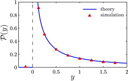
Figure 1: (Color online) The limiting probability density at $\alpha_{+}=\alpha=1/2$ and $\alpha_{-}>\alpha_{+}$. The solid blue line represents the theoretical result (82) and the simulation results (see Sec. VI) are indicated by red triangles.

IV.2.2 $\alpha\in(1,2)$, $\alpha_{+}\neq\alpha_{-}$, $l_{1}=0$

For these conditions, the limiting probability density in terms of the Laplace transform reads

$$\mathcal{P}(y)\!\! = \!\!\frac{H(\sigma y)}{\pi}\int_{0}^{\infty}dx\,e^{-|y|x}\frac{\sin(\phi_{+})\,x^{\alpha}}{1+2\cos(\phi_{+})\,x^{\alpha}+x^{2\alpha}}$$ (85)

$$\!\!+\,H(-\sigma y)\frac{1}{\alpha}\,e^{-|y|},$$

where $\phi_{+}=\pi(\alpha-1)$. It can be shown with the help of Eq. (83) that $\mathcal{P}(y)$ is normalized and

$$\mathcal{P}(y)|_{\sigma y\to+0}\!\! = \!\!\frac{1}{\pi}\int_{0}^{\infty}dx\frac{\sin(\phi_{+})x^{\alpha}}{1+2\cos(\phi_{+})x^{\alpha}+x^{2\alpha}}$$ (86)

$$= \!\!\frac{1}{\pi\alpha}\int_{0}^{\infty}dz\frac{\sin(\phi_{+})z^{1/\alpha}}{1+2\cos(\phi_{+})z+z^{2}}$$

$$= \!\!\frac{\sin(\phi_{+}/\alpha)}{\alpha\sin(\pi/\alpha)}.$$

Since $\phi_{+}=\pi(\alpha-1)$ and, in accordance with Eq. (85), $\mathcal{P}(y)|_{\sigma y\to-0}=1/\alpha$, we obtain

$$\mathcal{P}(0)=\mathcal{P}(y)|_{\sigma y\to\pm 0}=\frac{1}{\alpha}.$$ (87)

Thus, in contrast to the previous case, the limiting probability density is two-sided and is bounded at the origin. One branch of $\mathcal{P}(y)$, left if $\alpha_{-}>\alpha_{+}$ or right if $\alpha_{+}>\alpha_{-}$, is purely exponential, and the other is heavy-tailed (see also Sec. V). As before, the latter is concentrated on the semi-axis where the tail index is the smallest. Interestingly, the probability $\int_{0}^{\infty}dy\mathcal{P}[-\mathrm{sgn}(\sigma)y]=1/\alpha$ that $\sigma Y(\infty)<0$, i.e., the total probability defined by the exponential branch, is larger than $1/2$.

Figure 2 illustrates the behavior of $\mathcal{P}(y)$ in this case.

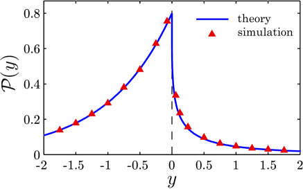
Figure 2: (Color online) The limiting probability density at $\alpha_{+}=\alpha=5/4$ and $\alpha_{-}>\alpha_{+}$. The solid line with an exponential left branch is obtained from Eq. (85) and triangles show the simulation results.

IV.2.3 $\alpha_{+}=\alpha_{-}=\alpha\in(0,1)$, $u_{+}\neq u_{-}$

From Eqs. (LABEL:limP_M3) and (81) it follows that

$$\mathcal{P}(y)\!\! = \!\!\frac{H(\epsilon y)}{\pi}\int_{0}^{\infty}dx\,e^{-|y|x}\frac{\sin(\phi_{+})x^{\alpha}}{1+2\cos(\phi_{+})x^{\alpha}+x^{2\alpha}}$$

$$\!\!+\frac{H(-\epsilon y)}{\pi}\int_{0}^{\infty}dx\,e^{-|y|x}\frac{\sin(\phi_{-})x^{\alpha}}{1+2\cos(\phi_{-})x^{\alpha}+x^{2\alpha}},$$

where the parameters $\phi_{+}$ and $\phi_{-}$ are given by Eq. (76). Since $\alpha<1$, one has $\mathcal{P}(0)=\infty$ and, using again Eq. (83), it can be verified that $\mathcal{P}(y)$ is normalized.

The comparison with the first case shows that, while the difference in the tail indexes $\alpha_{+}$ and $\alpha_{-}$ leads to a strongly asymmetric one-sided $\mathcal{P}(y)$, the difference in the parameters $u_{+}$ and $u_{-}$ (under condition that $\alpha_{+}=\alpha_{-}$) results in a less asymmetric two-sided $\mathcal{P}(y)$. According to Eq. (LABEL:limP_L3), both branches of the limiting probability density have heavy tails characterized by the same tail index $\alpha$ (see also Sec. V).

In this case, the behavior of $\mathcal{P}(y)$ is illustrated in Fig. 3.

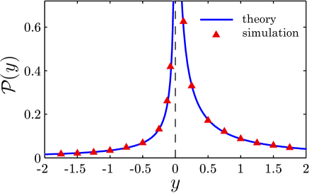
Figure 3: (Color online) The limiting probability density at $\alpha_{+}=\alpha_{-}=\alpha=1/2$ and $\epsilon=1/3$. The solid line and triangles represent the limiting probability density (LABEL:limP_L3) and simulation data, respectively.

IV.2.4 $\alpha_{+}=\alpha_{-}=\alpha\in(1,2)$, $u_{+}\neq u_{-}$, $l_{1}=0$

As in the previous section, the limiting probability density and the parameters $\phi_{+}$ and $\phi_{-}$ are determined by Eqs. (LABEL:limP_L3) and (76), respectively. The striking difference between the behavior of $\mathcal{P}(y)$ in these cases is that now $\mathcal{P}(0)<\infty$. To find $\mathcal{P}(0)$, we use Eq. (LABEL:limP_L3), which together with the standard integral (83) yields

$$\mathcal{P}(y)|_{\epsilon y\to\pm 0}=\frac{\sin(\phi_{\pm}/\alpha)}{\alpha\sin(\pi/\alpha)}.$$ (89)

Using Eq. (76), one obtains $\sin(\phi_{+}/\alpha)=\sin(\phi_{-}/\alpha)$, and so $\mathcal{P}(y)|_{\epsilon y\to\pm 0}=\mathcal{P}(0)$, where

$$\mathcal{P}(0)=\frac{1}{\alpha\sin(\pi/\alpha)}\cos\!\left\{\frac{1}{\alpha}\arctan\!\Big{[}|\epsilon|\tan\!\left(\frac{\pi\alpha}{2}\right)\!\Big{]}\!\right\}.$$ (90)

Comparing with the second case, we again observe that the difference in $\alpha_{+}$ and $\alpha_{-}$ causes more change in the behavior of branches of the limiting probability density than the difference in $u_{+}$ and $u_{-}$ at $\alpha_{+}=\alpha_{-}$.

The behavior of $\mathcal{P}(y)$ in this last case is shown in Fig. 4.

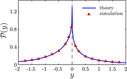
Figure 4: (Color online) The limiting probability density at $\alpha_{+}=\alpha_{-}=\alpha=5/4$ and $\epsilon=(\sqrt{2}-1)/(\sqrt{2}+1)$. As in the previous case, the solid line is obtained from Eq. (LABEL:limP_L3) and triangles indicate the simulation results.

IV.3 Representation of $\bm{\mathcal{P}(y)}$ in terms of the Fox $\bm{H}$ function

Since the Fox $H$ function is one of the most general special functions and many of its properties are well studied, it is also reasonable to express the limiting probability density in terms of this function. For this purpose, we first use the reflection formula Erd2 $\Gamma(z)\Gamma(1-z)=\pi/\sin(\pi z)$ to obtain

$$\frac{\sin\!\big{[}\phi(y)\frac{1-r}{\alpha}\big{]}}{\sin\!\big{(}\pi\frac{1-r}{\alpha}\big{)}}=\frac{\Gamma\big{(}\frac{1-r}{\alpha}\big{)}\Gamma\big{(}1-\frac{1-r}{\alpha}\big{)}}{\Gamma\big{[}\phi(y)\frac{1-r}{\pi\alpha}\big{]}\Gamma\big{[}1-\phi(y)\frac{1-r}{\pi\alpha}\big{]}}.$$ (91)

Then, substituting this relation into Eq. (66), one gets

$$\mathcal{P}(y)=\frac{1}{2\pi i\alpha}\int_{c-i\infty}^{c+i\infty}\!dr\frac{\Gamma(r)\Gamma\big{(}\frac{1-r}{\alpha}\big{)}\Gamma\big{(}1-\frac{1-r}{\alpha}\big{)}}{\Gamma\big{[}\phi(y)\frac{1-r}{\pi\alpha}\big{]}\Gamma\big{[}1-\phi(y)\frac{1-r}{\pi\alpha}\big{]}}|y|^{-r}.$$ (92)

On the other hand, the $H$ function can be defined in the form of a Mellin-Barnes integral as follows MSH :

$$H_{p,q}^{m,n}\!\left[y\Big{|}\begin{array}[]{lcl}(a_{p},A_{p})\\ (b_{q},B_{q})\end{array}\right]\!\!\! = \!\!H_{p,q}^{m,n}\!\left[y\Big{|}\begin{array}[]{lcl}(a_{1},A_{1}),\ldots,(a_{p},A_{p})\\ (b_{1},B_{1}),\ldots,(b_{q},B_{q})\end{array}\right]$$ (97)

$$= \!\!\frac{1}{2\pi i}\int_{L}dr\Theta_{r}y^{-r},$$ (98)

where

$$\Theta_{r}=\frac{\prod_{j=1}^{m}\Gamma(b_{j}+B_{j}r)\prod_{j=1}^{n}\Gamma(1-a_{j}-A_{j}r)}{\prod_{j=m+1}^{q}\Gamma(1-b_{j}-B_{j}r)\prod_{j=n+1}^{p}\Gamma(a_{j}+A_{j}r)},$$ (99)

$m,n,p,q$ are whole numbers, $0\leq m\leq q$, $0\leq n\leq p$, $a_{j}$ and $b_{j}$ are real or complex numbers, $A_{j},B_{j}>0$, $L$ is a suitable contour in the complex $r$-plane which separates the poles of the $\Gamma$ functions $\Gamma(b_{j}+B_{j}r)$ from the poles of the $\Gamma$ functions $\Gamma(1-a_{j}-A_{j}r)$, and the empty product is assumed to be equal to 1. Therefore, comparing Eq. (99) with the integrand in Eq. (92), we obtain the following representation of the limiting probability density through the $H$ function:

$$\mathcal{P}(y)=\frac{1}{\alpha}H_{2,3}^{2,1}\Bigg{[}|y|\bigg{|}\begin{array}[]{lcl}(1-\frac{1}{\alpha},\frac{1}{\alpha}),(1-\frac{\phi(y)}{\pi\alpha},\frac{\phi(y)}{\pi\alpha})\\[2.0pt] (0,1),(1-\frac{1}{\alpha},\frac{1}{\alpha}),(1-\frac{\phi(y)}{\pi\alpha},\frac{\phi(y)}{\pi\alpha})\end{array}\!\Bigg{]}.$$ (100)

Using this general formula, it is not difficult to find the corresponding representations for all four cases considered above. But here we focus on the first one for which Eq. (100) can be further simplified. Indeed, since in this case $\phi(y)=\phi_{\mathrm{sgn}(\sigma y)}$ with $\phi_{+}=\pi\alpha$ and $\phi_{-}=0$, from Eq. (100) and the reduction formula MSH

$$H_{p,q}^{m,n}\!\left[y\Big{|}\begin{array}[]{lcl}(a_{1},A_{1}),\ldots,(a_{p-1},A_{p-1}),(b_{1},B_{1})\\ (b_{1},B_{1}),\ldots,(b_{q},B_{q})\end{array}\right]$$ (103)

$$=H_{p-1,q-1}^{m-1,n}\!\left[y\Big{|}\begin{array}[]{lcl}(a_{1},A_{1}),\ldots,(a_{p-1},A_{p-1})\\ (b_{2},B_{2}),\ldots,(b_{q},B_{q})\end{array}\right]$$ (106)

($m\geq 1,p>n$) we obtain

$$\mathcal{P}(y)\!\! = \!\!\frac{H(\sigma y)}{\alpha}H_{2,3}^{2,1}\Bigg{[}|y|\bigg{|}\begin{array}[]{lcl}(1-\frac{1}{\alpha},\frac{1}{\alpha}),(0,1)\\[2.0pt] (0,1),(1-\frac{1}{\alpha},\frac{1}{\alpha}),(0,1)\end{array}\!\Bigg{]}$$ (109)

$$= \!\!\frac{H(\sigma y)}{\alpha}H_{1,2}^{1,1}\Bigg{[}|y|\bigg{|}\begin{array}[]{lcl}(1-\frac{1}{\alpha},\frac{1}{\alpha})\\[2.0pt] (1-\frac{1}{\alpha},\frac{1}{\alpha}),(0,1)\end{array}\!\Bigg{]}.$$ (112)

Then, using the relation

$$H_{p,q}^{m,n}\!\left[y\Big{|}\begin{array}[]{lcl}(a_{p},A_{p})\\ (b_{q},B_{q})\end{array}\right]\!=\frac{\chi}{y^{\lambda\chi}}H_{p,q}^{m,n}\!\left[y^{\chi}\Big{|}\begin{array}[]{lcl}(a_{p}+\lambda\chi A_{p},\chi A_{p})\\ (b_{q}+\lambda\chi B_{q},\chi B_{q})\end{array}\right]$$ (113)

($\chi>0,-\infty<\lambda<\infty$) with $\chi=\alpha$ and $\lambda=1/\alpha-1$, Eq. (112) can be reduced to

$$\mathcal{P}(y)=\frac{H(\sigma y)}{|y|^{1-\alpha}}\,H_{1,2}^{1,1}\!\left[|y|^{\alpha}\Big{|}\begin{array}[]{lcl}(0,1)\\ (0,1),(1-\alpha,\alpha)\end{array}\right]\!.$$ (114)

Finally, since this $H$ function is closely related to the generalized Mittag-Leffler function $E_{\alpha,\beta}(z)$ MSH ,

$$H_{1,2}^{1,1}\!\left[-z\Big{|}\begin{array}[]{lcl}(0,1)\\ (0,1),(1-\beta,\alpha)\end{array}\right]\!=E_{\alpha,\beta}(z)$$ (115)

($\alpha,\beta\,>0$), for the limiting probability density in the considered case, when $\alpha\in(0,1)$ and $\alpha_{+}\neq\alpha_{-}$, one gets

$$\mathcal{P}(y)=\frac{H(\sigma y)}{|y|^{1-\alpha}}\,E_{\alpha,\alpha}(-|y|^{\alpha}).$$ (116)

The usefulness of this result arises from that the Mittag-Leffler function is well studied (see, e.g., Ref. HMS and references therein). In particular, using the series definition of this function, $E_{\alpha,\beta}(z)=\sum_{n=0}^{\infty}z^{n}/\Gamma(\alpha n+\beta)$, we obtain

$$\mathcal{P}(y)=\frac{H(\sigma y)}{|y|^{1-\alpha}}\sum_{n=0}^{\infty}\frac{(-1)^{n}|y|^{\alpha n}}{\Gamma[\alpha(n+1)]}.$$ (117)

Remarkably, the limiting probability density (116) at $\alpha=1/2$ can be expressed through a simple complementary error function $\mathrm{erfc}(z)=(2/\sqrt{\pi})\int_{z}^{\infty}dxe^{-x^{2}}$. To show this, we first note that

$$E_{\alpha,\alpha}(-|y|^{\alpha})=-|y|^{1-\alpha}\frac{d}{d|y|}E_{\alpha,1}(-|y|^{\alpha}).$$ (118)

(This relation follows directly from the series representation of the Mittag-Leffler function.) Then, using the known result HMS $E_{1/2,1}(-z)=e^{z^{2}}\mathrm{erfc}(z)$, Eq. (116) at $\alpha=1/2$ can be written in the form

$$\mathcal{P}(y)=H(\sigma y)\left[\frac{1}{\sqrt{\pi|y|}}-e^{|y|}\mathrm{erfc}\big{(}\sqrt{|y|}\big{)}\right]\!.$$ (119)

The plot of this density function is shown in Fig. 1.

IV.4 Series representation of $\bm{\mathcal{P}(y)}$

We complete our study of alternative forms of the limiting probability density $\mathcal{P}(y)$ by determining its series representation. This representation can be useful, for example, for the numerical evaluation of $\mathcal{P}(y)$, especially in the vicinity of small $|y|$. Our starting point is the limiting probability density written in the form of inverse Mellin transform $\mathcal{P}(y)=(2\pi i)^{-1}\int_{c-i\infty}^{c+\infty}d\eta S(\eta)$ with

$$S(\eta)=\Gamma(1-\alpha\eta)\frac{\sin[\phi(y)\eta]}{\sin(\pi\eta)}|y|^{\alpha\eta-1}$$ (120)

[see the first line of Eq. (LABEL:limP_tr)]. To calculate the above integral, we close the integration path by a semicircle $C_{R}$ of a large radius $R$, which lies in the right half-plane of the complex variable $\eta$. If this semicircle does not cross any singularity of $S(\eta)$, then, using the Stirling approximation for the $\Gamma$ function Erd2 , it can be shown that the contribution of $C_{R}$ into the integral over the closed contour $L$ vanishes as $R\to\infty$. Therefore, from the residue theorem (see, e.g., Ref. AF ) we obtain $\mathcal{P}(y)=-\sum_{j}\mathrm{Res}(S,\eta_{j})$, where $\mathrm{Res}(S,\eta_{j})$ denotes the residue of $S(\eta)$ at $\eta=\eta_{j}$, the sum is taken over all isolated singularities (in our case poles) of $S(\eta)$ inside the contour $L$, and the sign $``-"$ accounts for the direction of $L$.

According to Eq. (120), the poles of $S(\eta)$ result from the first-order poles $\eta_{n}=n/\alpha$ ($n\geq 1$) of $\Gamma(1-\alpha\eta)$ and from the first-order poles $\eta_{m}=m$ ($m\geq 1$) of $1/\sin(\pi\eta)$. If $\alpha$ is irrational, then these sets of poles, $\{\eta_{n}\}$ and $\{\eta_{m}\}$, are not intersected, and hence all poles of $S(\eta)$ are also first-order. However, if $\alpha$ is rational, then some (or all if $\alpha=1$) poles from the set $\{\eta_{n}\}$ coincide with some (or all) poles from the set $\{\eta_{m}\}$, resulting in the appearance of the second-order poles of $S(\eta)$. Since the cases with irrational and rational values of $\alpha$ seem quite different, we consider them separately.

IV.4.1 Irrational values of $\alpha$

In this case, the limiting probability density is written as $\mathcal{P}(y)=-\sum_{n=1}^{\infty}\mathrm{Res}(S,n/\alpha)-\sum_{m=1}^{\infty}\mathrm{Res}(S,m)$. Therefore, taking into account that $\Gamma(1-\alpha\eta)|_{\eta=n/\alpha+\xi}\sim(-1)^{n}/[\alpha\Gamma(n)\xi]$ and $1/\sin(\pi\eta)|_{\eta=m+\xi}\sim(-1)^{m}/(\pi\xi)$ as $\xi\to 0$, and using the reflection formula $\Gamma(1-\alpha m)=\pi/[\Gamma(\alpha m)\sin(\pi\alpha m)]$, we readily find

$$\mathcal{P}(y)\!\! = \!\!\frac{1}{\alpha}\sum_{n=1}^{\infty}\frac{(-1)^{n-1}\sin[\phi(y)n/\alpha]}{\Gamma(n)\sin(\pi n/\alpha)}|y|^{n-1}$$ (121)

$$\!\!+\sum_{m=1}^{\infty}\frac{(-1)^{m-1}\sin[\phi(y)m]}{\Gamma(\alpha m)\sin(\pi\alpha m)}|y|^{\alpha m-1}.\quad$$

IV.4.2 Rational values of $\alpha$

Let us assume now that the tail parameter $\alpha$ is given by the irreducible fraction $\alpha=l/p$, where $l(\geq 1)$ and $p(\geq 1)$ are natural numbers satisfying the condition $l\leq 2p$. In this case, the first-order poles of $\Gamma(1-p\eta/l)$ with numbers $n=lk$ ($k=1,2,\ldots$) and the first-order poles of $1/\sin(\pi\eta)$ with numbers $m=pk$ are merged, and thus the poles of $S(\eta)$ at $\eta=pk$ become second-order. It is therefore convenient to represent the limiting probability density in the form

$$\mathcal{P}(y)\!\! = \!\!-\mspace{-20.0mu}\sum_{\begin{subarray}{c}n=1\\ (n\neq l,2l,\ldots)\end{subarray}}^{\infty}\mspace{-20.0mu}\mathrm{Res}(S,pn/l)-\mspace{-20.0mu}\sum_{\begin{subarray}{c}m=1\\ (m\neq p,2p,\ldots)\end{subarray}}^{\infty}\mspace{-20.0mu}\mathrm{Res}(S,m)$$ (122)

$$\!\!-\sum_{k=1}^{\infty}\mathrm{Res}(S,pk),$$

where the last sum is over all second-order poles of $S(k)$. Using the above results for the residues of $S(\eta)$ at the first-order poles and the asymptotic formula Erd2 $\Gamma(1-l\eta/p)|_{\eta=pk+\xi}\sim(-1)^{lk}(p/l)[\xi^{-1}-(l/p)\psi(lk)]/\Gamma(lk)$ ($\xi\to 0$) with $\psi(x)=d\ln\Gamma(x)/dx$ being the $\psi$ (or digamma) function, from Eq. (122) we obtain

$$\mathcal{P}(y)\!\! = \!\!\frac{p}{l}\mspace{-20.0mu}\sum_{\begin{subarray}{c}n=1\\ (n\neq l,2l,\ldots)\end{subarray}}^{\infty}\mspace{-20.0mu}\frac{(-1)^{n-1}\sin[\phi(y)pn/l]}{\Gamma(n)\sin(\pi pn/l)}|y|^{n-1}$$ (123)

$$\!\!+\mspace{-20.0mu}\sum_{\begin{subarray}{c}m=1\\ (m\neq p,2p,\ldots)\end{subarray}}^{\infty}\mspace{-24.0mu}\frac{(-1)^{m-1}\sin[\phi(y)m]}{\Gamma(lm/p)\sin(\pi lm/p)}|y|^{lm/p-1}$$

$$\!\!+\,\frac{1}{\pi}\sum_{k=1}^{\infty}\frac{(-1)^{pk+lk}}{\Gamma(lk)}\Big{(}[\psi(lk)-\ln|y|]\sin[\phi(y)pk]$$

$$\!\!-\,\frac{p}{l}\phi(y)\cos[\phi(y)pk]\Big{)}|y|^{lk-1}.$$

It should be noted that if $\alpha\in(0,1)$ and $\alpha_{+}\neq\alpha_{-}$ then the function $\phi(y)$ is given by Eq. (68). In this case Eqs. (121) and (123) are reduced to Eq. (117) leading to the Mittag-Leffler function representation (116). If $\alpha\in(1,2)$ and $\alpha_{+}\neq\alpha_{-}$ then $\mathcal{P}(y)$ can also be expressed in terms of the Mittag-Leffler function. Indeed, using Eq. (70) and the relations $\sum_{n=0}^{\infty}(\pm 1)^{n}|y|^{n}/n!=e^{\pm|y|}$ and $\sum_{n=1}^{\infty}|y|^{\alpha n}/\Gamma(\alpha n)=E_{\alpha,0}(|y|^{\alpha})=|y|^{\alpha}E_{\alpha,\alpha}(|y|^{\alpha})$, Eqs. (121) and (123) can easily be reduced to

$$\mathcal{P}(y)\!\! = \!\!H(\sigma y)\bigg{(}\frac{e^{|y|}}{\alpha}-|y|^{\alpha-1}E_{\alpha,\alpha}(|y|^{\alpha})\bigg{)}$$ (124)

$$\!\!+\,H(-\sigma y)\frac{e^{-|y|}}{\alpha}.$$

V SHORT- AND LONG-DISTANCE BEHAVIOR OF $\bm{\mathcal{P}(y)}$

The short-distance behavior of the limiting probability density $\mathcal{P}(y)$ is completely described by the series representations (121) and (123). To find the long-distance behavior of $\mathcal{P}(y)$, it is convenient to use its Laplace transform representation (81). According to Watson’s lemma AF , the asymptotic series expansion of $\mathcal{P}(y)$ at $|y|\to\infty$ is determined from the small-$x$ series expansion of the integrand function multiplied by $e^{|y|x}$. Therefore, using the series expansion Dw

$$\frac{\sin[\phi(y)]x^{\alpha}}{1+2\cos[\phi(y)]x^{\alpha}+x^{2\alpha}}=\sum_{n=1}^{\infty}(-1)^{n-1}\sin[\phi(y)n]x^{\alpha n}$$ (125)

($|x|<1$) and the standard integral PBM

$$\int_{0}^{\infty}dxe^{-|y|x}x^{\alpha n}=\frac{\Gamma(1+\alpha n)}{|y|^{1+\alpha n}},$$ (126)

from Eq. (81) one obtains

$$\mathcal{P}(y)\sim\frac{1}{\pi}\sum_{n=1}^{\infty}(-1)^{n-1}\sin[\phi(y)n]\frac{\Gamma(1+\alpha n)}{|y|^{1+\alpha n}}$$ (127)

as $|y|\to\infty$. For all cases of interest, we list below the main terms of $\mathcal{P}(y)$ at $|y|\to 0$ and $|y|\to\infty$.

1.    $\alpha\in(0,1)$, $\alpha_{+}\neq\alpha_{-}$

In this case, the two-valued function $\phi(y)$ is given by Eq. (68), $\mathcal{P}(y)|_{\sigma y<0}=0$, and thus Eqs. (117) and (127) lead to

$$\mathcal{P}(y)|_{\sigma y>0}\sim\frac{1}{\Gamma(\alpha)}\frac{1}{|y|^{1-\alpha}}$$ (128)

($|y|\to 0$) and to

$$\mathcal{P}(y)|_{\sigma y>0}\sim\frac{1}{\pi}\sin(\pi\alpha)\Gamma(1+\alpha)\frac{1}{|y|^{1+\alpha}}$$ (129)

($|y|\to\infty$), respectively.

2.    $\alpha\in(1,2)$, $\alpha_{+}\neq\alpha_{-}$, $l_{1}=0$

For these conditions, the function $\phi(y)$ is determined from Eq. (70), $\mathcal{P}(y)|_{\sigma y<0}=e^{-|y|}/\alpha$, and so Eqs. (121), (123) and (127) yield

$$\mathcal{P}(y)|_{\sigma y>0}\sim\frac{1}{\alpha}-\frac{1}{\Gamma(\alpha)}|y|^{\alpha-1}$$ (130)

as $|y|\to 0$ and

$$\mathcal{P}(y)|_{\sigma y>0}\sim-\frac{1}{\pi}\sin(\pi\alpha)\Gamma(1+\alpha)\frac{1}{|y|^{1+\alpha}}$$ (131)

as $|y|\to\infty$.

3.    $\alpha_{+}=\alpha_{-}=\alpha\in(0,1)$, $u_{+}\neq u_{-}$

Using Eq. (76), it can be straightforwardly shown that

$$\mathcal{P}(y)\sim\frac{1+\mathrm{sgn}(\epsilon y)|\epsilon|}{2\Gamma(\alpha)\sqrt{\epsilon^{2}+(1-\epsilon^{2})\cos^{2}(\pi\alpha/2)}}\frac{1}{|y|^{1-\alpha}}$$ (132)

as $|y|\to 0$ and

$$\mathcal{P}(y)\sim\frac{[1+\mathrm{sgn}(\epsilon y)|\epsilon|]\sin(\pi\alpha)\Gamma(1+\alpha)}{2\pi\sqrt{\epsilon^{2}+(1-\epsilon^{2})\cos^{2}(\pi\alpha/2)}}\frac{1}{|y|^{1+\alpha}}$$ (133)

as $|y|\to\infty$. In contrast to the first case, the limiting probability density has both left and right branches characterized by the same tail index $\alpha$.

4.    $\alpha_{+}=\alpha_{-}=\alpha\in(1,2)$, $u_{+}\neq u_{-}$, $l_{1}=0$

Finally, in this case we have

$$\mathcal{P}(y)\sim\mathcal{P}(0)-\frac{1+\mathrm{sgn}(\epsilon y)|\epsilon|}{2\Gamma(\alpha)\sqrt{\epsilon^{2}+(1-\epsilon^{2})\cos^{2}(\pi\alpha/2)}}|y|^{\alpha-1}$$ (134)

as $|y|\to 0$ and

$$\mathcal{P}(y)\sim-\frac{[1+\mathrm{sgn}(\epsilon y)|\epsilon|]\sin(\pi\alpha)\Gamma(1+\alpha)}{2\pi\sqrt{\epsilon^{2}+(1-\epsilon^{2})\cos^{2}(\pi\alpha/2)}}\frac{1}{|y|^{1+\alpha}}$$ (135)

as $|y|\to\infty$, where $\mathcal{P}(0)$ is given by Eq. (90). Note that at $\epsilon=0$ Eqs. (132)–(135) are reduced to those obtained in Ref. DYBKL for symmetric walks.

VI NUMERICAL SIMULATION OF $\bm{\mathcal{P}(y)}$

The determination of the limiting probability density $\mathcal{P}(y)$ by the numerical simulation is not a trivial problem. To understand why this is so, we first recall that $\mathcal{P}(y)$ is the probability density of the random variable $Y(t)=a(t)X(t)$ in the limit $t\to\infty$. In the simulation, however, we need to consider the behavior of the variable $Y(T)=a(T)X(T)$ and the corresponding probability density

$$\mathcal{P}_{T}(y)=\frac{1}{a(T)}\,P\!\left(\frac{y}{a(T)},T\right)$$ (136)

for some finite time $t=T$. To be sure that this probability density approaches $\mathcal{P}(y)$, the operating time $T$ must be large enough and, in principle, it should exceed the characteristic scale of waiting times. But in our case all fractional moments of the waiting-time density $p(\tau)$ do not exist and thus there is no finite time scale of $p(\tau)$. This means that for any finite $T$ there is always a non-negligible survival probability $V(T)=\int_{T}^{\infty}d\tau p(\tau)$ that the waiting time is larger than $T$. Therefore, the minimal value of $T$ is restricted only by the condition $a(T)\ll 1$ which is equivalent to $V(T)\ll 1$. Since $V(T)$ is a slowly varying function, it decreases with increasing of $T$ very slowly, and thus the operating time is expected to be very large. On the other hand, the larger is $T$ the larger is the average number $\overline{N}(T)$ of jumps occurring in the time interval $(0,T)$ [this is so because, according to Hug , $\overline{N}(T)\sim V^{-1}(T)$], and hence the larger is the computational time. Thus, the chosen value of the operating time $T$ must satisfy the condition $V(T)\ll 1$ and provide a reasonable computational time.

In our numerical simulations, we use the following waiting-time probability density:

$$p(\tau)=\frac{v\ln^{v}g}{(g+\tau)\ln^{1+v}(g+\tau)}$$ (137)

with $v>0$ and $g>1$. The main advantage of this density is that its distribution function $F_{p}(\tau)=\int_{0}^{\tau}d\tau^{\prime}p(\tau^{\prime})$ is calculated explicitly

$$F_{p}(\tau)=1-\frac{\ln^{v}g}{\ln^{v}(g+\tau)},$$ (138)

and thus the inverse function of $U=F_{p}(\tau)$ is given by $\tau=g^{(1-U)^{-1/v}}-g$. The last result permits us to use the inversion method Dev in accordance with which the random variables defined as

$$\tau_{n}=g^{(1-U_{n})^{-1/v}}-g,$$ (139)

where $n=1,2,\ldots$ and $U_{n}$ are random numbers uniformly distributed in the interval $[0,1]$, have the same probability density (137). This provides a simple way to generate the waiting times. For the simulations we choose $g=2,v=2$ and $T=10^{15}$ yielding $V(T)\approx 4\cdot 10^{-4}$.

Our choice of the jump density $w(\xi)$ is limited by two conditions. First, to verify the theoretical results, $w(\xi)$ must reproduce all possible cases considered earlier and, second, to simplify the generation of the jump lengths $\xi_{n}$, the corresponding distribution function $F_{w}(\xi)=\int_{-\infty}^{\xi}d\xi^{\prime}w(\xi^{\prime})$ must be invertible. These conditions are satisfied, for example, by the jump density

$$w(\xi)=\left\{\!\!\begin{array}[]{cl}\alpha_{-}c_{-}b_{-}^{\alpha_{-}}/(b_{-}-\xi)^{1+\alpha_{-}},&\xi<0\\[6.0pt] \alpha_{+}c_{+}b_{+}^{\alpha_{+}}/(b_{+}+\xi)^{1+\alpha_{+}},&\xi\geq 0.\end{array}\right.$$ (140)

Here, $b_{\pm}\in(0,\infty)$ and $c_{+}+c_{-}=1$ with $c_{+}$ and $c_{-}$ being the probabilities that $\xi\geq 0$ and $\xi<0$, respectively. It can be easily shown from Eq. (140) that

$$F_{w}(\xi)=\left\{\!\!\begin{array}[]{cl}c_{-}b_{-}^{\alpha_{-}}/(b_{-}-\xi)^{\alpha_{-}},&\xi<0\\[6.0pt] 1-c_{+}b_{+}^{\alpha_{+}}/(b_{+}+\xi)^{\alpha_{+}},&\xi\geq 0,\end{array}\right.$$ (141)

and thus the jump lengths can be determined as

$$\xi_{n}=\left\{\!\!\begin{array}[]{cl}-b_{-}(c_{-}/U_{n})^{1/\alpha_{-}}+b_{-},&U_{n}<c_{-}\\[6.0pt] b_{+}[c_{+}/(1-U_{n})]^{1/\alpha_{+}}-b_{+},&U_{n}\geq c_{-}.\end{array}\right.$$ (142)

Now we are ready to describe the procedure for calculating $\mathcal{P}_{T}(y)$. According to the definition, the particle starts to walk at time $t=0$ from the position $X(0)=0$. At the first step, the waiting time $\tau_{1}$ and the jump length $\xi_{1}$ are generated using Eqs. (139) and (142), respectively. If $\tau_{1}\leq T$, then the particle position becomes $X(\tau_{1})=\xi_{1}$, and we can go to second step that consists in generating new random numbers $\tau_{2}$ and $\xi_{2}$. If at the $n$th step the condition $\sum_{i=1}^{n}\tau_{i}\leq T$ is violated, then the walk is stopped at the previous step, i.e., the scaled position $Y(t)$ of the first particle at $t=T$ is assumed to be $Y(T)=a(T)\sum_{i=1}^{n-1}\xi_{i}$ [$Y(T)=0$ at $n=1$], where the scaling function $a(T)$ can be calculated using an appropriate theoretical formula. Determining $Y(T)$ for $N$ particles, we can evaluate the limiting probability density as follows: $\mathcal{P}_{T}(y)=N_{\Delta y}/N$, where $N_{\Delta y}$ is the number of particles with $Y(T)\in[y,y+\Delta y)$. In all our simulations we set $N=10^{5}$ and $\Delta y=10^{-1}$; the other parameters are listed below.

1.    $\alpha\in(0,1)$, $\alpha_{+}\neq\alpha_{-}$

In this case, the limiting probability density $\mathcal{P}(y)$ depends only on the minimal tail index $\alpha$ [see, e.g., Eq. (69)]. But to determine the approximate probability density $\mathcal{P}_{T}(y)$ by the proposed procedure, all the parameters in Eqs. (137) and (140) must be specified. In addition to the parameters mentioned above, we choose $\alpha=\alpha_{+}=1/2$, $c_{+}=2/3$, $b_{+}=1$ and $\alpha_{-}=3/4$, $c_{-}=1/3$, $b_{-}=1$. With these parameters, Eq. (34) yields $a(T)\approx 1.2\cdot 10^{-7}$ and the simulated values of $\mathcal{P}_{T}(y)$, marked by red triangles, are shown in Fig. 1.

2.    $\alpha\in(1,2)$, $\alpha_{+}\neq\alpha_{-}$, $l_{1}=0$

Since the first moment of the probability density (140) is given by

$$l_{1}=\frac{c_{+}b_{+}}{\alpha_{+}-1}-\frac{c_{-}b_{-}}{\alpha_{-}-1},$$ (143)

($\alpha_{\pm}>1$) the condition $l_{1}=0$ implies that the parameters of $w(\xi)$ satisfy the condition $c_{+}b_{+}/(\alpha_{+}-1)=c_{-}b_{-}/(\alpha_{-}-1)$. In particular, if $\alpha=\alpha_{+}=5/4$, $c_{+}=5/22$, $b_{+}=1$ and $\alpha_{-}=37/20$, $c_{-}=17/22$, $b_{-}=1$, then $c_{+}b_{+}/(\alpha_{+}-1)=c_{-}b_{-}/(\alpha_{-}-1)=10/11$, $a(T)\approx 1.8\cdot 10^{-3}$, and the results of simulation of $\mathcal{P}_{T}(y)$ are shown in Fig. 2.

3.    $\alpha_{+}=\alpha_{-}=\alpha\in(0,1)$, $u_{+}\neq u_{-}$

According to Eq. (140) and the asymptotic formula (16), the parameters $u_{\pm}$ are expressed through the parameters of $w(\xi)$ as follows: $u_{\pm}=\alpha_{\pm}c_{\pm}b_{\pm}^{\alpha_{\pm}}$. Keeping in mind that $\alpha_{+}=\alpha_{-}=\alpha$ and $u_{+}\neq u_{-}$, i.e., $c_{+}b_{+}^{\alpha_{+}}\neq c_{-}b_{-}^{\alpha_{-}}$, we choose $\alpha=1/2$, $c_{+}=2/3$, $b_{+}=1$ and $c_{-}=1/3$, $b_{-}=1$. For these parameters, $u_{+}=1/3$, $u_{-}=1/6$ (i.e., $\epsilon=1/3$), $a(T)\approx 9.3\cdot 10^{-8}$ and the simulated results are shown in Fig. 3.

4.    $\alpha_{+}=\alpha_{-}=\alpha\in(1,2)$, $u_{+}\neq u_{-}$, $l_{1}=0$

In this case, the conditions $u_{+}\neq u_{-}$ and $l_{1}=0$ are reduced to $c_{+}b_{+}^{\alpha}\neq c_{-}b_{-}^{\alpha}$ and $c_{+}b_{+}=c_{-}b_{-}$, respectively. Choosing $\alpha=5/4$, $c_{+}=1/5$, $b_{+}=5$ and $c_{-}=4/5$, $b_{-}=5/4$, one gets $u_{+}=5^{5/4}/4\approx 1.87$, $u_{-}=(5/4)^{5/4}\approx 1.32$ [i.e., $\epsilon=(\sqrt{2}-1)/(\sqrt{2}+1)\approx 0.17$], $a(T)\approx 5.2\cdot 10^{-4}$ and the simulated values of $\mathcal{P}_{T}(y)$ are shown in Fig. 4.

As is seen from these figures, the numerical results are in very good agreement with our theoretical predictions. It is also worth to note that the proposed numerical method reproduces all the other limiting probability densities, Eqs. (25), (49) and (58), and can easily be extended to study the CTRWs, including coupled ones, in higher dimensions.

VII CONCLUSIONS

We have studied in detail the long-time behavior of the decoupled CTRWs characterized by superheavy-tailed distributions of waiting times and asymmetric heavy-tailed distributions of jump lengths. The main attention is devoted to introducing the scaled particle position and deriving its limiting probability density $\mathcal{P}(y)$. Using the Montroll-Weiss equation in the Fourier-Laplace space and the asymptotic properties of the waiting-time and jump-length distributions, we have found both the scaling function, which determines the scaled position, and the representation of $\mathcal{P}(y)$ in terms of the inverse Fourier transform. It has been shown that while the scaling function depends on the parameters describing the asymptotic behavior of both waiting-time and jump-length distributions, the limiting probability density is completely characterized by the parameters of the latter distribution. Among these parameters, the main role plays the smallest tail index $\alpha$.

To get more information about the limiting probability density, we have derived a number of alternative representations of $\mathcal{P}(y)$. The representation of $\mathcal{P}(y)$ in terms of the inverse Mellin transform is important from a theoretical point of view (all other representations considered in the paper follow from this one) and permits to determine the intervals of $\alpha$ where $\mathcal{P}(y)$ exhibits qualitatively different behavior. We have also obtained the limiting probability density in terms of the Fox $H$ function. The importance of this representation is that the $H$ function is well studied and many of the special functions can be considered as its particular cases. In particular, we have shown that if the tail indexes of the jump density are different and $\alpha\in(0,1)$ then $\mathcal{P}(y)$ is expressed through the generalized Mittag-Leffler function. Then, using the limiting density in terms of the Laplace transform, we have analytically demonstrated that $\mathcal{P}(y)$ is non-negative, has a maximum value at the origin, and monotonically decreases (or equals zero) as $|y|$ increases. We have also derived the series representation of $\mathcal{P}(y)$ which, in the case when the tail indexes of the jump density are different and $\alpha\in(1,2)$, has been used to obtain the limiting density in terms of the Mittag-Leffler function. Moreover, the series representation of $\mathcal{P}(y)$ together with its Laplace transform representation have permitted us to completely describe the short- and long-distance behavior of the limiting probability density. It has been shown, in particular, that the tail index of $\mathcal{P}(y)$ is equal to the lowest tail index of the jump probability density.

Finally, we have developed a numerical method for calculating the limiting probability density. This method, which deals with the statistics of the scaled particle position at large times, has been applied to calculate $\mathcal{P}(y)$ in all cases of interest. It has been shown that the simulation results for the limiting probability density are in excellent agreement with our theoretical predictions.

Appendix A Fractional equation for $\bm{\mathcal{P}(y)}$

Let us define the Riesz-Feller space-fractional derivative ${}_{y}D_{\theta}^{\gamma}$ of order $\gamma$ and skewness $\theta$ as (see, e.g., Ref. MLP )

$$\mathcal{F}\{{}_{y}D_{\theta}^{\gamma}f(y)\}=-e^{i\mathrm{sgn}(\kappa)\pi\theta/2}|\kappa|^{\gamma}f_{\kappa},$$ (144)

where $\gamma\in(0,2]$, $|\theta|\leq\min\{\gamma,2-\gamma\}$, and $\mathcal{F}\{f(y)\}=\int_{-\infty}^{\infty}dye^{i\kappa y}f(y)=f_{\kappa}$. Then, using this definition and Eq. (35), one gets

$$\mathcal{F}\{{}_{y}D_{-2\varphi/\pi}^{\alpha}\mathcal{P}(y)\}\!\! = \!\!-e^{-i\mathrm{sgn}(\kappa)\varphi}|\kappa|^{\alpha}\mathcal{P}_{\kappa}$$ (145)

$$= \!\!-\Phi(\kappa)\mathcal{P}_{\kappa}.$$

Finally, taking into account that $\mathcal{F}\{\delta(y)\}=1$ and, as it follows from Eq. (21), $\mathcal{F}\{\mathcal{P}(y)\}=[1+\Phi(\kappa)]^{-1}$, the fractional equation for the limiting probability density $\mathcal{P}(y)$ can be written in the form

$${}_{y}D_{-2\varphi/\pi}^{\alpha}\mathcal{P}(y)=\mathcal{P}(y)-\delta(y).$$ (146)

References

- (1) H. Scher and E. W. Montroll, Phys. Rev. B 12, 2455 (1975).
- (2) R. Metzler and J. Klafter, Phys. Rep. 339, 1 (2000).
- (3) D. ben-Avraham and S. Havlin, Diffusion and Reactions in Fractals and Disordered Systems (Cambridge University Press, Cambridge, 2000).
- (4) R. Klages, G. Radons, and I. M. Sokolov, eds., Anomalous Transport: Foundations and Applications, (Wiley-VCH, Berlin, 2008).
- (5) D. Brockmann, L. Hufnagel, and T. Geisel, Nature 439, 462 (2006).
- (6) C. Song, T. Koren, P. Wang, and A.-L. Barabási, Nat. Phys. 6, 818 (2010).
- (7) E. Scalas, R. Gorenflo, F. Mainardi, Physica A 284, 376 (2000).
- (8) J. Masoliver, M. Montero, and G. H. Weiss, Phys. Rev. E 67, 021112 (2003).
- (9) E. Scalas, Physica A 362, 225 (2006).
- (10) J. Masoliver, M. Montero, J. Perelló, and G. H. Weiss, Physica A 379, 151 (2007).
- (11) A. Helmstetter and D. Sornette, Phys. Rev. E 66, 061104 (2002).
- (12) L. Palatella, P. Allegrini, P. Grigolini, V. Latora, M. S. Mega, A. Rapisarda, and S. Vinciguerra, Physica A 338, 201 (2004).
- (13) E. W. Montroll and G. H. Weiss, J. Math. Phys. 6, 167 (1965).
- (14) J. Klafter and G. Zumofen, J. Phys. Chem. 98, 7366 (1994).
- (15) E. Barkai, Phys. Rev. E 63, 046118 (2001); Chem. Phys. 284, 13 (2002).
- (16) G. Germano, M. Politi, E. Scalas, and R. L. Schilling, Phys. Rev. E 79, 066102 (2009).
- (17) J. K. E. Tunaley, J. Stat. Phys. 11, 397 (1974).
- (18) M. F. Shlesinger, J. Klafter, and Y. M. Wong, J. Stat. Phys. 27, 499 (1982).
- (19) H. Weissman, G. H. Weiss, and S. Havlin, J. Stat. Phys. 57, 301 (1989).
- (20) M. Kotulski, J. Stat. Phys. 81, 777 (1995).
- (21) M. M. Meerschaert and H. P. Scheffler, J. Appl. Prob. 41, 623 (2004).
- (22) S. Havlin and G. H. Weiss, J. Stat. Phys. 58, 1267 (1990).
- (23) J. Dräger and J. Klafter, Phys. Rev. Lett. 84, 5998 (2000).
- (24) A. V. Chechkin, J. Klafter, and I. M. Sokolov, Europhys. Lett. 63, 326 (2003).
- (25) S. I. Denisov and H. Kantz, Europhys. Lett. 92, 30001 (2010).
- (26) S. I. Denisov, H. Kantz, and P. Hänggi, J. Phys. A: Math. Theor. 43, 285004 (2010).
- (27) S. I. Denisov and H. Kantz, Eur. Phys. J. B 80, 167 (2011).
- (28) S. I. Denisov and H. Kantz, Phys. Rev. E 83, 041132 (2011).
- (29) S. I. Denisov, S. B. Yuste, Yu. S. Bystrik, H. Kantz, and K. Lindenberg, Phys. Rev. E 84, 061143 (2011).
- (30) W. Feller, An Introduction to Probability Theory and its Applications, 2nd ed., Vol. 2, Chap. XIII (Wiley, New York, 1971).
- (31) A. P. Prudnikov, Yu. A. Brychkov, and O. I. Marichev, Integrals and Series, Vol. 1 (Gordon & Breach, New York, 1986).
- (32) L. Debnath and D. Bhatta, Integral Transforms and their Applications, 2nd ed., Chap. 8 and Appendix B-6 (Chapman & Hall/CRC Press, New York, 2007).
- (33) A. Erdélyi, ed., Tables of Integral Transforms, Bateman Manuscript Project, Vol. 1 (McGraw-Hill, New York, 1954).
- (34) A. Erdélyi, ed., Higher Transcendental Functions, Bateman Manuscript Project, Vol. 1 (McGraw-Hill, New York, 1953), Chap. 1.
- (35) R. B. Paris and D. Kaminski, Asymptotics and Mellin-Barnes Integrals, Eq. (3.3.12) (Cambridge University Press, Cambridge, 2001).
- (36) A. M. Mathai, R. K. Saxena, and H. J. Haubold, The H-Function: Theory and Applications, Chap. 1 (Springer, New York, 2010).
- (37) H. J. Haubold, A. M. Mathai, and R. K. Saxena, J. Appl. Math. 2011, 298628 (2011).
- (38) M. J. Ablowitz and A. S. Fokas, Complex Variables: Introduction and Applications (Cambridge University Press, Cambridge, 2003).
- (39) H. B. Dwight, Tables of Integrals and Other Mathematical Data, 4th ed., Eq. (417.4) (Macmillan, New York, 1961).
- (40) B. D. Hughes, Random Walks and Random Environments, Vol. 1, Chap. 5.1.4 (Clarendon Press, Oxford, 1995).
- (41) L. Devroye, Non-Uniform Random Variate Generation, Chap. II.2 (Springer, New York, 1986).
- (42) F. Mainardi, Yu. Luchko, and G. Pagnini, Fract. Calc. Appl. Anal. 4(2), 153 (2001).