Geosynchronous Microlens Parallaxes

Abstract

I show that for a substantial fraction of planets detected in a space-based survey, it would be possible to measure the planet and host masses and distances, if the survey satellite were placed in geosynchronous orbit. Such an orbit would enable measurement of the microlens parallax $\pi_{\rm E}$ for events with moderately low impact parameters, $\beta\lesssim 0.05$, which encompass a disproportionate share of planetary detections. Most planetary events yield a measurement of the angular Einstein radius $\theta_{\rm E}$. Since the host mass is given by $M=\theta_{\rm E}/\kappa\pi_{\rm E}$ where $\kappa$ is a constant, parallax measurements are the crucial missing link. I present simple analytic formulae that enable quick error estimates for observatories in circular orbits of arbitrary period and semi-major axis, and arbitrary orientation relative to the line of sight. The method requires photometric stability of $\sim 10^{-4}$ on $\sim 1$ orbit timescales. I show that the satellite data themselves can provide a rigorous test of the accuracy of the parallax measurements in the face of unknown systematics and stellar variability, even at this extreme level.

1 Introduction

Microlens planet detections routinely yield the planet-star mass $q=m/M$, but since the host star is generally very difficult to observe, the host mass $M$ (and so the planet mass $m$) and the system distance $D_{L}$ usually remain undetermined. In principle, one can determine these quantities from the microlensing event itself, provided the angular Einstein radius $\theta_{\rm E}$ and the microlens parallax $\pi_{\rm E}$ are both measured (Gould, 1992)

$$M={\theta_{\rm E}\over\kappa\pi_{\rm E}},\quad\pi_{\rm rel}=\theta_{\rm E}\pi_{\rm E},\quad\kappa\equiv{4G\over c^{2}{\rm AU}}=8.1{{\rm mas}\over M_{\odot}},$$ (1)

where $\pi_{\rm E}={\rm AU}/\tilde{r}_{\rm E}$ is the ratio of the Earth’s orbit to the Einstein radius projected on the observer plane, and $\pi_{\rm rel}\equiv{\rm AU}[D_{L}^{-1}-D_{S}^{-1}]$ is the lens-source relative parallax, with $D_{S}$ generally being known from direct observation of the source.

To date, $\theta_{\rm E}$ has been measured in the majority of planetary events, even though it is rarely ($\sim 0.1\%$) measured in ordinary events. This is because planets are detected when the source passes near or over a caustic induced by the planet, which yields a measurement of the source size relative to the Einstein radius.

Hence, if a method could be found to measure $\pi_{\rm E}$ for a large fraction of events, the information returned from microlensing planet searches would be radically improved. The microlens parallax is actually a vector ${\mbox{\boldmath$\pi$}}_{\rm E}$, with the direction being that of the lens-source relative motion. It can in principle be measured either from the ground (Gould, 1992), by combining space-based and ground-based observations (Refsdal, 1966), or from space alone (Honma, 1999).

When I proposed the pure ground-based method (Gould, 1992), I illustrated it with an event that lasted 4 years, so that the lightcurve oscillated annually around the standard microlensing form. In practice, such 4-year events are never seen, but ${\mbox{\boldmath$\pi$}}_{\rm E}$ can be measured from less regular features in shorter events. However, typical events have timescales $t_{\rm E}\sim 20\,$days, so that the great majority are too short to permit a measurement. Honma (1999) proposed a purely space-based method using Hubble Space Telescope (HST) observations. Since the HST orbital period is only 1.5 hours, the oscillations are obviously much shorter than $t_{\rm E}$. However, the HST orbital radius is only $R_{\oplus}$, whereas typically $\tilde{r}_{\rm E}\sim 1-10\,{\rm AU}$. Hence, the oscillations would typically be minuscule. To overcome this obstacle, Honma (1999) proposed that the observations should be made during caustic crossings, which he showed dramatically increase the strength of the signal. However, alerting HST to imminent caustic crossings is extremely difficult, more so for planetary events, and in fact such measurements have never been carried out, nor even attempted. The ground-space combination originally proposed by Refsdal (1966) remains feasible in principle, but each event must be observed very frequently (Gaudi & Gould, 1997), implying a huge space-craft investment. Recently, Gould & Yee (2012) showed that a much simpler and cheaper ground-space approach was feasible for high-magnification events, but these constitute a small subset.

Here I show that a single survey satellite in geosynchronous orbit is a near-optimal solution to this problem. As in my original proposal, oscillations are induced on a standard microlensing lightcurve, but since these have periods of one day rather than one year, they are shorter than the event. The amplitude of the oscillations is 6.6 times larger than those of the Honma (1999) proposed HST observations. Moreover, no special warning system is required. It is true that this approach only works for moderately high-magnification ($A\gtrsim 10$) events, but these are more sensitive to planets than more typical events (Gould & Loeb, 1992). Hence, this approach can yield parallaxes for a large fraction of planetary events. Moreover, such a geosynchronous survey satellite is a very real possibility. The Decadal Survey Committee (2010) report recommended a Wide Field Infrared Space Telescope (WFIRST) as its highest priority. A large fraction of the observing time would be devoted to microlensing planet searches. Although originally recommended for L2 orbit, a geosynchronous orbit is now being actively considered. Hence, it is most timely to investigate the implications of such an orbit for microlensing parallaxes.

2 Analytic Treatment of Single-Observatory Parallax

Consider an observatory in circular orbit with period $P$ and semi-major axis $a$. If this is an Earth orbit, these two quantities are obviously related, but here I begin with the general case. Let the microlensing target be at a latitude $\lambda$ with respect to the plane of this orbit, so that the projected semi-minor axis is $b=a\sin\lambda$. I then normalize these axes to an AU

$${\epsilon}_{\parallel}\equiv{\epsilon}={a\over{\rm AU}};\quad{\epsilon}_{\perp}={a\sin\lambda\over{\rm AU}};$$ (2)

Now consider that continuous observations of a microlensing event are made at a rate $N$ per Einstein timescale $t_{\rm E}$, with signal-limited flux errors

$$\sigma^{2}=\sigma_{0}^{2}A.$$ (3)

This condition is not as restrictive as may first appear. We are only concerned with scaling of the errors when the source is relatively highly magnified, so that this form need not hold all the way down to baseline, where sky and blending may be important. Let the lens pass the source on its right at an angle $\theta$ relative to the major projected axis of the satellite orbit, with impact parameter $\beta$ (in units of $\theta_{\rm E}$). Then the lens-source separation vector $\bf u$ (in units of $\theta_{\rm E}$) is given by

$${\bf u}=(\tau\cos\theta-\beta\sin\theta+{\epsilon}_{\parallel}\pi_{\rm E}\cos(\omega t+\phi),\tau\sin\theta+\beta\cos\theta+{\epsilon}_{\perp}\pi_{\rm E}\sin(\omega t+\phi))$$ (4)

where $\tau\equiv(t-t_{0})/t_{\rm E}$, $t_{0}$ is the time of closest approach, $\omega=2\pi/P$, and $\phi$ is the orbit phase relative to peak. By definition, ${\mbox{\boldmath$\pi$}}_{\rm E}=(\pi_{{\rm E},\parallel},\pi_{{\rm E},\perp})=\pi_{\rm E}(\cos\theta,\sin\theta)$. Hence,

$${{\partial}u\over{\partial}\pi_{{\rm E},\parallel}}={{\epsilon}_{\parallel}\tau\cos(\omega t+\phi)+{\epsilon}_{\perp}\beta\sin(\omega t+\phi)\over u},\qquad{{\partial}u\over{\partial}\pi_{{\rm E},\perp}}={-{\epsilon}_{\parallel}\beta\cos(\omega t+\phi)+{\epsilon}_{\perp}\tau\sin(\omega t+\phi)\over u}$$ (5)

The magnification is given by (Einstein, 1936)

$$A={u^{2}+2\over u\sqrt{u^{2}+4}},\qquad{{\partial}\ln A\over{\partial}u}=-{8\over u(u^{2}+2)(u^{2}+4)},$$ (6)

so that the derivatives of the flux with respect to the parallax parameters are

$${{\partial}F\over{\partial}\pi_{{\rm E},\parallel}}=F_{s}{{\partial}\ln A\over{\partial}u}A{{\partial}u\over{\partial}\pi_{{\rm E},\parallel}},\qquad{{\partial}F\over{\partial}\pi_{{\rm E},\perp}}=F_{s}{{\partial}\ln A\over{\partial}u}A{{\partial}u\over{\partial}\pi_{{\rm E},\perp}},$$ (7)

where $F_{s}$ is the unmagnified source flux. In order to make a Fisher-matrix analysis, I first assume that the magnification does not change much over an orbit. This will ultimately restrict the result to events for which $t_{\rm eff}\equiv\beta t_{\rm E}>P$. I will discuss the more general case further below. I then evaluate the mean contribution to the Fisher matrix, averaged over one orbit

$${1\over\sigma^{2}}\langle\biggl{(}{{\partial}F\over{\partial}\pi_{{\rm E},\parallel}}\biggr{)}^{2}\rangle={F_{s}^{2}\over\sigma_{0}^{2}}\langle\biggl{(}{{\partial}u\over{\partial}\pi_{{\rm E},\parallel}}\biggr{)}^{2}\rangle A\biggl{(}{{\partial}\ln A\over{\partial}u}\biggr{)}^{2}={F_{s}^{2}\over 2\sigma_{0}^{2}}{64({\epsilon}_{\parallel}^{2}\tau^{2}+{\epsilon}_{\perp}^{2}\beta^{2})\over u^{5}(u^{2}+4)^{5/2}(u^{2}+2)}$$ (8)

$${1\over\sigma^{2}}\langle\biggl{(}{{\partial}F\over{\partial}\pi_{{\rm E},\perp}}\biggr{)}^{2}\rangle={F_{s}^{2}\over 2\sigma_{0}^{2}}{64({\epsilon}_{\perp}^{2}\tau^{2}+{\epsilon}_{\parallel}^{2}\beta^{2})\over u^{5}(u^{2}+4)^{5/2}(u^{2}+2)}$$ (9)

$${1\over\sigma^{2}}\langle{{\partial}F\over{\partial}\pi_{{\rm E},\parallel}}{{\partial}F\over{\partial}\pi_{{\rm E},\perp}}\rangle={F_{s}^{2}\over 2\sigma_{0}^{2}}{64({\epsilon}_{\perp}^{2}-{\epsilon}_{\parallel}^{2})\tau\beta\over u^{5}(u^{2}+4)^{5/2}(u^{2}+2)}$$ (10)

and so obtain the inverse covariance matrix by integrating over all observations

$$B={NF_{s}^{2}\over\sigma_{0}^{2}}\left(\matrix{{\epsilon}_{\parallel}^{2}G_{2}+{\epsilon}_{\perp}^{2}G_{0}&0\cr 0&{\epsilon}_{\perp}^{2}G_{2}+{\epsilon}_{\parallel}^{2}G_{0}\cr}\right)$$ (11)

where

$$G_{n}(\beta)\equiv\int_{0}^{\infty}dx{64\,x^{n}\beta^{2-n}\over(x^{2}+\beta^{2})^{5/2}(x^{2}+\beta^{2}+4)^{5/2}(x^{2}+\beta^{2}+2)}.$$ (12)

In the limit $\beta\ll 1$, it is straightforward to show that

$$G_{0}(\beta)\rightarrow{2\over 3}\beta^{-2},\quad G_{2}(\beta)\rightarrow{1\over 3}\beta^{-2}.$$ (13)

Figure 1 shows that this approximation holds quite well for $\beta\lesssim 0.1$ (i.e., $A_{\rm max}\gtrsim 10$). Using this approximation, we obtain,

$$\left(\matrix{\sigma(\pi_{{\rm E},\parallel})\cr\sigma(\pi_{{\rm E},\perp})}\right)=\sqrt{3\over N}{\sigma_{0}\over F_{s}}{\beta\over\epsilon}\left(\matrix{(1+2\sin^{2}\lambda)^{-1/2}\cr(2+\sin^{2}\lambda)^{-1/2}}\right)$$ (14)

Since the ratio of the quantities in the right-hand vector is never greater than $\sqrt{2}$ (and is $\sqrt{3/2}$ for $\lambda=30^{\circ}$, which is typical of Galactic bulge fields and an equatorial orbit), the parallax error is reasonably well characterized by the harmonic rms of these two values,

$$\sigma(\pi_{\rm E})\simeq\biggl{(}{B_{11}+B_{22}\over 2}\biggr{)}^{-1/2}=0.023\biggl{(}{N\over 10000}\bigg{)}^{-1/2}\biggl{(}{1+\sin^{2}\lambda\over 1.25}\bigg{)}^{-1/2}\biggl{(}{\sigma_{0}/F_{s}\over 0.01}\bigg{)}\biggl{(}{\beta\over 0.05}\bigg{)}\biggl{(}{{\epsilon}\over 6.6\,R_{\oplus}/{\rm AU}}\bigg{)}^{-1}$$ (15)

3 Application to WFIRST

The fiducial values in Equation (15) are plausible for a WFIRST style mission. For example, a continuous sequence of 3-minute exposures yields $N\sim 10000$ for a $t_{\rm E}=20\,$day event. A large fraction of sources would have 1% errors in such an exposure, whether continuous or co-added. Note that the formula does not really specify $\sigma_{0}$ and $N$ separately, but just $\sigma_{0}/\sqrt{N}$. Moreover, for typical $t_{\rm E}=20\,$day events and a $P=1\,$day orbit, the assumptions of the derivation basically apply for $\beta=0.05$, i.e., $t_{\rm eff}=\beta t_{\rm E}=P$. Of course, the integral in Equation (12) goes to infinity, while the observations do not, but the overwhelming contribution to this integral is from a few $t_{\rm eff}$ near peak. The fiducial parallax error in Equation (15) is quite adequate to measure the mass and distance of disk lenses but somewhat marginal for bulge lenses. For example, for $M=0.5\,M_{\odot}$, a typical disk lens at $D_{L}=4\,$kpc has $\pi_{\rm E}\sim 0.18$, but a typical bulge lens at $D_{S}-D_{L}=0.75\,$kpc has $\pi_{\rm E}\sim 0.06$. At the very least, however, such a measurement would distinguish between bulge and disk lenses.

4 Systematics and Stellar Variability

Naively, Equation (15) appears to require “effective errors” of $N^{-1/2}\sigma_{0}/F_{s}\sim 10^{-4}$, which must be achieved in the face of both astrophysical and instrumental effects. In particular, it would seem to challenge the systematics limit for real crowded-field photometry, even from space. However, what is actually required is not control of systematics to this level, but only control of systematic effects that correlate with orbital phase. This requirement is still not trivial for geosynchronous orbit because of phase-dependent temperature variations, but it is not as intractable as vetting all systematic errors at this level.

Nothing is known about stellar variability at this level in $H$ (likely WFIRST passband). Even Kepler has only a handful of stars for which it can make measurements of this precision in its optical passband (Fig. 4 of McQuillan et al. 2012). However, again what is relevant is not variability per se, but variability on 1-day timescales, and McQuillan et al. (2012) report that FGK stars typically vary on $>5$-day timescales. Moreover, most forms of intrinsic variability are very subdued in $H$ band relative to the optical. See Gould et al. (2013) for a spectacular example of this in a microlensing event. Finally, McQuillan et al. (2012) find that variability declines with increasing proper motion (so presumably age), and the bulge is mostly much older than the disk, though perhaps not entirely (Bensby et al., 2013)

5 Rigorous Test of Parallax Accuracy

One would nevertheless like a rigorous test that undetectable variability and systematic effects are not corrupting the results. Fortunately the satellite data themselves provide such a test. Gould et al. (1994) showed that even very short microlensing events yield “one-dimensional parallaxes” from the asymmetry in the lightcurve induced by the Earth’s (approximately constant) acceleration toward the Sun. That is, $\pi_{{\rm E},\odot,\parallel}$ is well constrained while $\pi_{{\rm E},\odot,\perp}$ is very poorly constrained. Normally, such 1-D parallaxes are not considered useful because the amplitude of $\pi_{\rm E}$ (and so $M$) is also poorly constrained. However, in the present case these 1-D parallaxes serve two very important functions. Figure 2 shows the lightcurve of a simulated event with 72 days of observations centered on the Vernal Equinox in each of 5 years, similar to the anticipated schedule of WFIRST. The event is assumed to have the fiducial parameters from Equation (15): $t_{\rm E}=20\,$days, $\beta=0.05$, $N^{-1/2}(\sigma_{0}/F_{s})=10^{-4}$, with $t_{0}$ right at the Vernal Equinox. The lower panel shows the difference between this event as observed from a geosynchronous orbit, and the same event observed from an inertial platform. Note that since the orbit is equatorial, $(\pi_{{\rm E},\parallel},\pi_{{\rm E},\perp})=(\pi_{{\rm E},E},\pi_{{\rm E},N})$, i.e., the components of ${\mbox{\boldmath$\pi$}}_{\rm E}$ in the East and North directions projected on the sky. The event is at $(\alpha,\delta)=$(18:00:00,-30:00:00), and is assumed to have a parallax $(\pi_{{\rm E},E},\pi_{{\rm E},N})=(0.1,0.1)$. The oscillations near peak are due to the satellite’s orbital motion, while the asymmetries in the wings are from the Earth’s orbit. The latter are much larger, but yield only 1-D information. This is illustrated in Figure 3, which shows the error ellipses due to 1) Earth-only, 2) satellite-only, 3) Earth+satellite. Also shown is the result of the analytic calculation (which assumed observations extending to infinity). Note that there are two sets of solutions in each case, corresponding to the ($\beta\rightarrow-\beta$) degeneracy (Smith et al., 2003; Gould, 2004).

The first point is that if $\pi_{{\rm E},E}$ as derived from geosynchronous parallax agrees with the much more precise value derived from the Earth’s orbit, then one can have good confidence in $\pi_{{\rm E},N}$, for which there is no direct test. This is true on an event by event basis, but more true for the ensemble of parallax measurements.

The second point is that these two parallax measurements will be automatically combined in the fit to any lightcurve, which means that $\pi_{{\rm E},E}$ will be much better determined than $\pi_{{\rm E},N}$. Depending on the relative values of these two components, this may add important information in some cases.

Finally, the ensemble of geosynchronous measurements of $\pi_{{\rm E},E}$ provides a test of the accuracy of the 1-D Earth-orbit measurement of this quantity from the wings of the event. This is important because the source stars may show variability on 10-day timescales, even if they do not vary on 1-day timescales.

Using techniques similar to those used to derive Equation (14), it is straightforward to show that the 1-D parallax error due to Earth acceleration for short, relatively high-magnification events (and infinite observations) is

$$\sigma(\pi_{{\rm E},\odot,\parallel})=\sqrt{3\over N}{\sigma_{0}\over F_{s}}\biggl{(}{t_{\rm E}\over 58\,{\rm day}}\biggr{)}^{-2}\eta^{-1},$$ (16)

where 58 days is one radian of the Earth’s orbit and $\eta$ is the projected Earth-Sun separation in AU at time $t_{0}$. Since $\eta\sim 1$ for bulge observations made during the equinoxes, the ratio of geosynchronous-to-Earth parallax errors is

$${\sigma(\pi_{{\rm E}})_{\rm geosynch}\over\sigma(\pi_{{\rm E},\odot,\parallel})_{\rm Earth}}\simeq 20\biggl{(}{t_{\rm E}\over 20\,{\rm day}}\biggr{)}^{2}\,{\beta\over 0.05}={t_{\rm E}\over 1\,\rm day}\,{\beta t_{\rm E}\over 1\,\rm day}.$$ (17)

Since the effective $\beta t_{\rm E}\gtrsim P=1\,$day, this implies that the Earth-orbit parallax will essentially always yield a precise check on the geosynchronous parallax in one direction.

6 Discussion

The derivation underlying Equation (15) breaks down for $t_{\rm eff}\lesssim P$: the errors continue to decline with falling $\beta$, but no longer linearly. They also become dependent on the orientation and phase of the orbit in a much more complicated way. From the present perspective, the main point is that the formula with $\beta\rightarrow P/t_{\rm E}$ provides an upper limit on the errors for events with yet higher peak magnification.

Next, the errors derived here assume a point-lens event. However, since the observations would be near-continuous, it is likely that caustic crossings or near approaches would be captured. As pointed out by Honma (1999) such caustic effects can significantly enhance the signal.

Another feature of these (and most) parallax measurements is that they work better at low mass, simply because $\pi_{\rm E}\propto M^{-1/2}$ is bigger. Space-based microlensing measurements have the potential to directly detect the lens when it is more massive (so, typically, brighter). For example, as the lens and source separate after (or before) the event, their joint light becomes extended and the centroids of the blue and red light separate (if the source and lens are different colors). These effects allowed Bennett et al. (2006) and Dong et al. (2009) to measure the host masses in two different planetary events using followup HST data. Because geosynchronous parallax works better at low mass, while photometric/astrometric methods work better at high mass, they are complementary.

Finally, I note that such parallaxes would be of great interest in non-planetary events as well. Without $\theta_{\rm E}$, such measurements do not yield masses and distances, but they do serve as important inputs into Bayesian estimates of these quantities. Moreover, since the direction of ${\mbox{\boldmath$\pi$}}_{\rm E}$ is the same as that of the lens-source relative proper motion ${\mbox{\boldmath$\mu$}}_{\rm rel}$, a parallax measurement provides an important constraint when trying to detect/measure the source-lens displacement away from the event. If the magnitude $\mu_{\rm rel}$ can be measured from these data, then so can $\theta_{\rm E}=\mu_{\rm rel}t_{\rm E}$, which in turn yields the mass and distance.

Figure 1: Functional forms of $G_{0}(\beta)$ and $G_{2}(\beta)$ relative to the limiting forms given by Equation (13). These approximations are excellent for $\beta<0.05$ and very good for $\beta<0.1$.

Figure 2: Simulated lightcurve of event with $t_{\rm E}=20\,$days, $\beta=0.05$, $t_{0}$ at the Vernal Equinox, and parallax $\pi_{{\rm E},N}=\pi_{{\rm E},E}=0.1$, observed from a geosynchronous equatorial orbit. The error bars are binned by day for display but the observations are assumed many times per day.

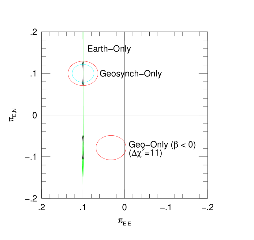
Figure 3: Error ellipses ($1\,\sigma$) for the event shown in Figure 2 using Earth-orbit-only (green), geosynchronous-only (red) and combined (black) information. The lightcurve asymmetry (Fig. 2) due to the Earth’s orbit yields only 1-D parallax information, but this serves as a critical check on the accuracy of the geosynchronous-orbit parallax. The secondary minimum at $\pi_{{\rm E},N}\sim-0.07$ is due to $(\beta\rightarrow-\beta)$ degeneracy. In this example, it is disfavored by $\Delta\chi^{2}=11$ based on geosynchronous data and by 15 based on all data. The analytic error estimate (based on infinite data) is shown in cyan.

References

- Bennett et al. (2006) Bennett, D.P., Anderson, J., Bond, I.A., Udalski, A., & Gould A. 2006, ApJ, 647, L171
- Bensby et al. (2013) Bensby, T. et al. 2013, A&A, in press (arXiv:1211.6848)
- Decadal Survey Committee (2010) Committee for a Decadal Survey in Astronomy and Astrophysics 2010, New Worlds, New Horizons, Washington DC: National Academies Press
- Dong et al. (2009) Dong, S., et al. 2009, ApJ, 695, 970
- Einstein (1936) Einstein, A. 1936, Science, 84, 506
- Gaudi & Gould (1997) Gaudi, B.S. & Gould, A. 1997, ApJ, 477, 152
- Gould (1992) Gould, A. 1992, ApJ, 392, 442
- Gould (2004) Gould, A. 2004, ApJ, 606, 319
- Gould & Loeb (1992) Gould, A. & Loeb, A. 1992, ApJ, 396, 104
- Gould et al. (1994) Gould, A., Miralda-Escudé, J. & Bahcall, J.N. 1994, ApJ, 423, L105
- Gould & Yee (2012) Gould, A. & Yee, J.C. 2012, ApJ, 755, L17
- Gould et al. (2013) Gould, A. et al. 2013, ApJ, in press (arXiv:1210.6045)
- Honma (1999) Honma, M. 1999, ApJ, 517, L35
- McQuillan et al. (2012) McQuillan, A., Algrain, S., & Roberts, S. 2012, A&A, 539
- Refsdal (1966) Refsdal, S. 1966, MNRAS, 134, 315
- Smith et al. (2003) Smith, M., Mao, S., & Paczyński, B. 2003, MNRAS 339, 925