Homogeneous Interpolation and Some Continued Fractions
Abstract.
We prove: if , there is no curve of degree passing through general points with multiplicity in . Similar results are given for other special values of . Our bounds can be naturally written as certain palindromic continued fractions.
2010 Mathematics Subject Classification:
Primary 14C20; Secondary 14J26, 14N05.1. Introduction
Denote by the linear system of degree curves in passing through general points with multiplicity at least . For , Nagata’s conjecture ([10]) predicts that is empty if . The statement is clear if is a square, but remains widely open otherwise. A refined conjecture due to Harbourne-Hirschowitz further predicts that in fact is non-special, i.e. of expected dimension , where
is the virtual dimension of . We refer to ([3],[4],[5],[6]) for background on the problem and some recent results.
In this paper we prove:
Main Theorem.
Let be a non-square positive integer. Write with . Assume that either:
-
i)
, or
-
ii)
, is even, .
If the linear system is nonempty, then , where
Note that is a palindromic continued fraction with rational coefficients. The value is well-known to be sharp ([10]). The next few cases are , , , and . Since , our bound for ten points is stronger than the bound obtained by Eckl ([6]) and Ciliberto et. al. ([3]).
In the case we have a more refined result (Prop. 12.2). As a striking application, we are able show that the linear system is non-special (with ).
The proof of the Theorem consists of two degenerations. First, we specialize the general points in to general points on a fixed curve of degree . The problem is naturally reduced to an interpolation problem on a ruled surface where is a semistable rank 2 vector bundle of degree on . Second, we specialize the points in to a curve of self-intersection (in general, this step requires a deformation of the underlying surface ). The methods in this paper extend our previous attempt in [11]. We were greatly influenced by the work of Ciliberto-Miranda in [5].
The paper is organized as follows. In Section 2 we introduce a Basic Lemma that will be useful throughout the paper. In Section 3 we give background on ruled surfaces and elementary transforms. In Section 4 we perform the first degeneration and obtain a certain weak bound on for any . The construction is formalized in the next two sections. In Section 7 we sketch the proof of the Main Theorem. In each subsequent section we verify the theorem for specific values of . In Section 12 we prove a certain refinement of the Main Theorem. In Appendix A we review the indecomposable elliptic ruled surface of degree 1. Appendix B has some auxiliary results on continued fractions.
Notation and Conventions
We work over . Following EGA IV.4, for given a subscheme we denote by the conormal sheaf of . For any coherent sheaf on , we denote .
Acknowledgments
The author is grateful to E. Cotterill for valuable comments and suggestions for improving the paper.
2. Basic Lemma
The following elementary lemma is the key ingredient to several arguments in this paper.
Lemma 2.1 (Basic Lemma).
Let be a nonsingular curve embedded in a nonsingular projective variety . Let be an effective divisor on . Denote , the multiplicity of vanishing of along . Then, there is a natural injective morphism of sheaves , where is the conormal bundle of in .
Proof.
Let be the blowup of . Then , where is the exceptional divisor of and is the strict transform of . We have , the tautological line bundle on . So, is naturally a subsheaf of (also, it is a subbundle iff has no vertical components). ∎
We can use the lemma to give a lower bound on based on the “local data” . This takes a particularly simple form if is a semistable vector bundle. Recall that, by definition, a vector bundle on a curve is semistable if and only if for any subsheaf , we have . Here we denote . For background on semistability, see e.g. [12].
Corollary 2.2.
In the above setting, suppose that is semistable. Then
Proof.
This follows from Basic Lemma together with the fact that, for any , is semistable of slope ([12], Thm. 10.2.1). ∎
3. Ruled Surfaces and Semistability
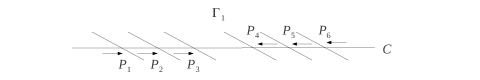
In this section we give some background on ruled surfaces and elementary transforms. Our reference is ([8], Ch. V). Let be a smooth curve of genus and let be a ruled surface over . Let be a minimal section of , i.e. a section of minimal self-intersection. The invariant is the degree of (this differs by sign from Hartshorne’s notation). We have:
Lemma 3.1.
Let be a rank 2 vector bundle on . Consider the ruled surface . The following are equivalent:
-
(a)
is semistable;
-
(b)
;
-
(c)
for any effective divisor of , we have .
Proof.
(a) (b) See [8], Exercise V.2.8.
(b) (c) Let be a minimal section of . Suppose . Let be an effective divisor. Then, where (this follows from [8], Prop. V.2.20 if and Prop. 21 if ). Hence .
(c) (b) is obvious. ∎
If with semistable, we will also say that the surface is semistable. By the lemma above, is semistable if and only if is of degree .
3.1. Elementary Transforms
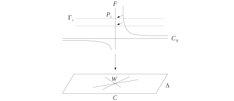
Let be a ruled surface over and let be a point on . We can create a new ruled surface by applying an elementary transform at ([8], Example V.5.7.1). We recall the construction. Denote by be the fiber of through . Let be the blowup of and let be the strict transform of in . Finally, let be the contraction of the (-1)-curve in (see Fig. 1).
Similarly, we can define elementary transforms for vector bundles. In the setting above, suppose that where is a rank 2 vector bundle on . Consider the short exact sequence
where the map on the right is just the evaluation map at . The kernel is again a rank 2 vector bundle on . We can identify with the surface constructed above.
The following lemma describes the behavior of semistability under elementary transforms.
Lemma 3.2.
Let be a semistable ruled surface. Let be a general point on a fixed fiber of (the fiber need not be general). Let be the ruled surface obtained from by applying an elementary transform at . Then is semistable, unless is the trivial ruled surface.
Proof.
If is not semistable, there exists a section of with . Denote by be the strict transform of in . Since is semistable, we have . It follows that passes through and . Since is a general point on a fiber , it follows that . ∎
4. First Degeneration
We introduce the first degeneration. The method in this section extends author’s previous work in [11]. As an application we prove Theorem 4.1 below. We are unaware if the result has appeared previously in the literature in this form.
Theorem 4.1.
Let be a non-square positive integer. Write with . Assume that either: (i) is even, or (ii) . If the linear system is nonempty, then , where
In particular, the theorem applies for and and any .
Example 4.2.
Example 4.3.
If , we have , which is also sharp. The linear system has a unique section, namely the union of six conics each passing through 5 of the 6 points (Loc. cit.).
Proof of the Theorem.
Assume is nonempty. The idea is to specialize the general points in to a smooth curve of degree and then apply Basic Lemma to estimate the multiplicity of vanishing of a general curve in along .
Step 1. Let be the open unit disk over and let . We view as a relative plane over . For any , denote the fiber . Fix a smooth curve of degree . We have the following split exact sequence
where and . Consider the ruled surface
Let be the section of corresponding to the short exact sequence above. Note that and .
Step 2. Choose any set of distinct points on (here we do not require the points to be general). Next, we construct a set of relative points in specializing to in a general way. Denote by the images of in . Thus, each is a general point on the fiber above .
Let be the blowup of the relative points and let denote the corresponding exceptional divisors. Denote by the strict transform of in . We have the following short exact sequence:
We have and , where
is a line bundle of degree on . The short exact sequence corresponds to a certain element
Next, consider the ruled surface
We identify with the section of corresponding to the above exact sequence. Note that and .
The conormal bundles and are related by elementary transforms at the points :
Similarly, the ruled surfaces and are related by elementary transforms as on Fig. 1 (the intermediate surface will play a role later in Section 5).
Step 3. We claim:
Lemma 4.4.
Let be an arbitrary element. Then can be realized in the above way, for some specialization of points to .
Proof.
The idea is to consider the construction in Step 2 in reversed order. Start with any extension
and let . As before, we identify with the section of corresponding to the above exact sequence. Next, we construct the vector bundle by applying elementary transforms at the points on :
Let and let be as on Fig. 1. It follows that is realized as an extension
Now, the key observation is that
so the above extension is trivial. This allows us to identify with , and so with . Finally, we choose the relative points to pass through in . This identifies with , and so with . ∎
Corollary 4.5.
If the specialization of to is general enough, the conormal bundle is semistable of slope .
This follows from Lemma 4.4 and the following general fact:
Lemma 4.6.
Let be a curve of genus . Let be a line bundle on of degree . Assume that either: (i) is even, or (ii) . Then, a general element corresponds to a semistable rank 2 vector bundle on .
Proof.
Step 4. We complete the proof of the theorem. Since is nonempty by assumption, there is a flat family of curves , where is a nontrivial section of . We are interested in estimating , which of course is the same as where is the image of in . Obviously,
By Lemma 4.5 and Cor. 2.2, we have:
Combining and , we get:
One can easily check that this is equivalent to the inequality in the theorem. See also Lemma B.1(a) in the Appendix. ∎
5. Reduction of Interpolation Problems to Ruled Surfaces
We formalize some results from the previous section. Our result here is Theorem 5.5 which will be used through the rest of the paper.
Notation 5.1.
A marked surface is simply a surface together with distinct points on .
Notation 5.2.
Let be a marked ruled surface over . For any integers and a line bundle of degree on , we denote the line bundle
on the blowup at the points , with exceptional divisors . Here we denote .
Lemma 5.3.
We have
where and is the genus of .
Proof.
Notation 5.4.
Let be a smooth curve, a line bundle on and let corresponding to an extension
We denote by
the ruled surface and we identify with the section determined by the short exact sequence. Note that and .
The following theorem allows to reduce interpolation problems on to certain interpolation problems on ruled surfaces.
Theorem 5.5.
Let be a non-square positive integer. Write with and . Consider the linear system for some positive integers and . Fix a smooth curve of degree in . Let be a marked ruled surface where:
-
•
is any line bundle of degree on ;
-
•
is any element;
-
•
are distinct points on such that
Then, for any , we have
where:
-
•
of degree ;
-
•
;
-
•
.
The following lemma justifies our definition of :
Lemma 5.6.
In the setting of the theorem, we have , where is the strict transform of in .
Proof.
This is an easy computation. We have:
The lemma follows. ∎
Proof of Theorem.
We will use the same construction as in the proof of Theorem 4.1.
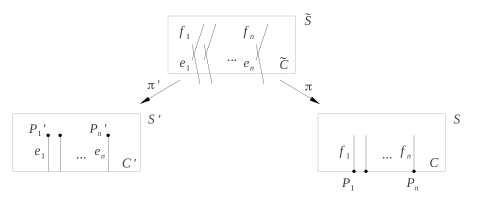
Step 1. Consider the threefold . We identify with a curve on . Given , we specialize the relative points to as in Lemma 4.4. As before, let be the blowup of the , and let be the strict transform of in . We have the short exact sequence
where and . By construction, the above extension corresponds to . In particular, , where is the ruled surface we started with.
Step 2. Consider the threefold obtained from by first blowing up (with exceptional divisor ), followed by blowing up the strict transforms of the relative points (with exceptional divisors ). We view as a flat family with general fiber . The special fiber is the union of two surfaces meeting transversely along . 111We denote by , resp. , the same curve in viewed as a divisor in , resp. .
This construction is related to the construction in Step 1 as follows. Let be the threefold obtained from by blowing up (with exceptional divisor ). Then, can be obtained from by applying (-1)-transfers to the exceptional curves as on Fig. 2 (see also [4], Section 4.1). The induced map coincides with the corresponding map on Fig. 1.
Step 3. For a given , consider the following line bundle on :
We view as a flat family of line bundles with general fiber . The special fiber is described by the following short exact sequence:
where
Lemma 5.7.
We have:
Proof.
The line bundle has the following properties:
From Lemma 5.6, has the same properties. It follows that . ∎
To complete the proof of the theorem, take cohomology in :
The restriction is surjective. Hence, the coboundary map . The theorem now follows from the semicontinuity principle applied to . ∎
Corollary 5.8.
Assume the above setting.
-
(a)
For any , we have:
-
(b)
For any (hence ), we have:
Proof.
(a) This follows from the short exact sequence and the fact that is a constant function of .
(b) This follows from (a). ∎
Corollary 5.9.
Suppose the linear system is nonempty. Then is nonempty with .
Proof.
Consider the long exact cohomology sequence associated to . If , the restriction is an isomorphism. The claim follows. ∎
6. Families of Ruled Surfaces
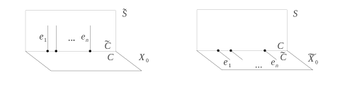
We can use the degeneration technique from the previous section to reduce an interpolation problem on to an interpolation problem on a certain ruled surface . We would like to perform further degenerations to study the later problem. Our first goal is to define an object which is a relative analogue of . We conclude with a technical result (Prop. 6.4) which will be used in Sections 10 and 13. As usual, denotes the open unit disk over .
Notation 6.1.
Let be a torsion-free sheaf of rank 1 on . Assume that where is invertible and is the ideal sheaf of a l.c.i. zero-dimensional subscheme (possibly ). Let be an element corresponding to an extension
such that is locally free. We denote by
the relative ruled surface together with the subscheme defined by the above exact sequence. In particular, is a divisor of with .
We will assume that is supported on . In applications, will be reduced; however, everything we say in this section holds in the more general setting.
Lemma 6.2.
In the above setting, the projection is just the blowup of . Denote by the exceptional divisor of . Then .
Proof.
Since is invertible, which is exactly the definition of a blowup. The rest is clear. ∎
Consider the following question: given as above, which elements correspond to a locally free extension ? Clearly, if , then is locally free and so any will do. In the general case, we have:
Proposition 6.3.
Let be as above. Then, there is a natural exact sequence
Moreover, we have:
(a) .
(b) The extension corresponding to is locally free if and only if generates the sheaf .
Proof.
See [7], Chapter 2, p. 36–37. The exact sequence follows from the local-to-global spectral sequence
Note that where is the projection. In particular, for .
(a) Ibid., Lemma 7 (note that the isomorphisms are not canonical).
(b) Ibid., Theorem 8. ∎
Consider a relative ruled surface . For any , is a ruled surface over where arises as an extension
We have . For a general , the subscheme is a section of . On the special fiber, we have , where is a section of and is the vertical component of . If , we will say that is a degenerate section of .
Next, we will show that any degenerate section can be smoothed, in the following sense.
Proposition 6.4.
Let be as above, with is supported on . Let
be any extension, with locally free. Then, the exact sequence can be extended to
with locally free on .
Proof.
Consider the commutative diagram with exact rows:
Note that where . Therefore, . It follows that the bottom row of the diagram splits. Now, the map on the left factors through
which is surjective. The map on the right is just the restriction
which is also surjective. By the Short Five Lemma, the map in the middle is surjective as well. Hence, any given extension can be lifted to . The resulting is locally free by Prop. 6.3(b). ∎
7. Main Result – Overview
The following theorem was announced in the introduction. The proof will occupy the rest of the paper. We will consider a certain refinement in Section 12.
Main Theorem.
Let be a non-square positive integer. Write with . Assume that either:
-
i)
, or
-
ii)
, is even, .
If the linear system is nonempty, then .
The proof of the theorem consists of the four steps outlined below.
7.1. Setup
7.2. Degeneration
We will construct a relative marked ruled surface over such that the general fiber satisfies the assumptions of Theorem 5.5, i.e.:
-
•
is a line bundle on of relative degree .
-
•
lie on . We denote by the projection of under .
-
•
For general, we have on .
We now describe the special fiber . We assume that is semistable. Next, we assume that there is a smooth (possibly disconnected) curve on with the following two properties:
-
•
meets transversely at distinct points points ;
-
•
.
This determines uniquely the numerical class of :
where . In particular, a necessary condition for the existence of is that .
Let where each is a smooth irreducible curve, with for . Since and is semistable, lies on the boundary of the effective cone of (this follows from Lemma 3.2). Therefore, for some with (in fact, in applications we will always have ).
7.3. Semistability
Denote by the blowup of and let be the corresponding exceptional divisors. Denote by the strict transform of . We make the following hypothesis:
-
•
for each , the conormal bundle is semistable of slope .
7.4. Invariants
Assuming the construction above can be realized, we complete the proof of the theorem. Consider the line bundle
on the blowup , where
-
•
;
-
•
of relative degree .
-
•
.
By construction, there is a flat family of curves in , where is a section of . Denote by the projection of in . The following is a key computation:
Lemma 7.1.
Define Then
Proof.
Using the fact that , and , we find:
Finally, substitute and . ∎
To complete the proof of the theorem, we will estimate in two ways. First, there is an obvious upper bound which comes from the numerical class of :
Since , this becomes:
By Basic Lemma and the semistability hypothesis, we have:
i.e.
From and , and using , we get:
It turns out that this is equivalent to the inequality in the theorem. We will check this explicitly for specific values of . For the general case, see Lemma B.1(b) in the Appendix.
8. Eight Points
We verify Main Theorem in the case . The value is well-known to be sharp (see example below). We include this case for illustration purposes.
8.1. Setup
Since , we take to be a smooth conic in . The line bundle on is of degree . Consider an extension
corresponding to a general . It follows that
Hence, . We identify with the section of corresponding to the short exact sequence. It follows that where is a horizontal section of .
8.2. Degeneration
Let and . We identify with the special fiber of . We take on , where each is a general horizontal section of . Let . Next we specialize the eight relative points to in a general way.
8.3. Semistability
Let be the blowup of along the relative points . We have to show that, for each , the conormal bundle is semistable (of slope 1). Denote by the image of in the corresponding . Then, is obtained from by performing elementary transforms at the points . If the specialization is general enough, the points do not belong to the same horizontal section of . It follows that , which is semistable of slope 1.
8.4. Invariants
Denote . By symmetry, . Since , we have the following upper bound:
The lower bound from Basic Lemma is:
Combining and , we get:
q.e.d.
The bound is sharp:
Example 8.1.
9. Ten Points
Here we prove Main Theorem for points.
9.1. Setup
Since , we take to be a smooth cubic in . Fix a point on such that
For example, we can take to be a Weierstrass point of (however, later in Section 12 we will require that ). Let which is of degree . Since , there is a unique nontrivial extension
The surface is an indecomposable elliptic ruled surface of degree 1 (see Appendix A for background). The short exact sequence determines a minimal section of which we identify with the curve .
9.2. Degeneration
Let and . We identify with the special fiber of . Next, we take , where each is a general section of the pencil . By Prop. A.1, each is a smooth elliptic curve. Denote . Note that Since , we have
Finally, we specialize the ten relative points in to in a general way such that
for any .
9.3. Semistability
We claim that, for each , is semistable (of slope 1). Denote by the image of in . Now, is obtained from by performing elementary transforms at the points . If the specialization is general enough, the points do not belong to the same horizontal section of . It follows that , which is semistable of slope 1.
9.4. Invariants
Denote . By symmetry, . Since , we have the following upper bound:
The lower bound from Basic Lemma is:
From and , we get:
q.e.d.
10. Eleven Points
We prove Main Theorem for points. This is the first time when we study an interpolation problem by deforming the underlying surface itself.
10.1. Setup
As before, is a smooth cubic in . Fix a point on such that Let be any line bundle of degree on . It is easy to see that for a general , the ruled surface is decomposable of degree 0. Denote by , , the two minimal sections of . It follows that .
10.2. Degeneration
We will construct a relative marked ruled surface such that:
-
•
The special fiber is simply .
-
•
The special section ; here is a horizontal section of and is the fiber of above .
-
•
The relative points on are such that on , for general .
-
•
Each limit point is a general point on .
The construction is done as follows. First, we choose relative points in specializing to in a general way. Let
Since , it follows that
Consider the following short exact sequence on :
By Prop. 6.4, the sequence can be extended to
with locally free. Let and . Hence . Now, is just the blowup of with exceptional divisor . Finally, we take to be the strict transform of in .
10.3. Semistability
We take where is the horizontal section of through (see Fig. 4). Consider the blowup at the relative points . We claim that for each , is indecomposable of degree 1 (hence semistable of slope 1/2). First, we will show that is indecomposable of degree 0.
We will need some deformation theory. Let be the ring of dual numbers. Let viewed as an infinitesimal deformation of over . We will say that a section of is (infinitesimally) unobstructed if and only if can be extended to a subscheme of flat over .
Lemma 10.1.
Assume the above setting.
-
(a)
is unobstructed if and only if the following short exact sequence splits:
-
(b)
Suppose there are 3 disjoint horizontal sections of that are unobstructed. Then, is an infinitesimally trivial deformation, i.e. . In particular, any section of is unobstructed.
-
(c)
is obstructed.
Proof.
(a) This is clear.
(b) We have where . For any , the embedding induces a surjective morphism where is a line bundle on . By Nakayama’s lemma, for any , the induced map is an isomorphism. Hence , i.e. .
(c) Consider the short exact sequence
where and . Since , it is clear that . Now consider the short exact sequence from part (a):
where and . It follows that is indecomposable of degree 0. Hence, is obstructed. ∎
Part (c) of the lemma implies that is not an infinitesimally trivial deformation. By part (b) and by symmetry, is obstructed for any . It follows that the conormal bundle is indecomposable of degree 0.
Denote by the image of in . Clearly, does not belong to the unique minimal section of (because meets transversely). Finally, is obtained from by performing an elementary transform at . It follows that is indecomposable of degree 1.
10.4. Invariants
Denote . By symmetry, . Since , we have the following upper bound:
The lower bound from Basic Lemma is:
Combining and , we get:
This completes the proof for eleven points.
Remark 10.2.
It might be also profitable to study the behavior of along the fiber . We have , which follows from the split exact sequence
with and . The fact that is unstable causes certain multiplicity and tangency conditions on the limit curve at the point . A more careful analysis of the situation is beyond of the scope of this paper.
11. Twelve Points
In this section we prove Main Theorem for . This case is similar to .
11.1. Setup
As before, is a smooth cubic in . Fix a point on such that . Take which is of degree . It is easy to see that for a general , is an indecomposable elliptic ruled surface of degree 1. It follows that where is a minimal section of .
11.2. Degeneration
Let and . We identify with the special fiber of . Take where each is a general section of the pencil . In particular, . Let and . It follows that
Next, we specialize in to in a general way such that
for any .
11.3. Semistability
We have to show that if the specialization of the points is general enough, the conormal bundle is semistable (of slope 3). Since semistability is an open property ([9], Thm. 2.8), it suffices to describe a particular specialization for which is semistable. This is not hard. In fact, we claim that we can specialize the points in such a way that
and similarly for . This can be achieved by moving the triples of points “in parallel” while being assigned to the same section of the pencil .
11.4. Invariants
Denote . By symmetry, . Since , we have the following upper bound:
The lower bound from Basic Lemma is:
Combining and , we get:
This completes the proof for twelve points.
12. A Refinement
Here we prove a certain refinement of the Main Theorem in the case of and points. We work in the setting of the previous sections. The idea is to show that, under some additional assumptions, the inequality can be replaced by a stronger inequality . First, we have:
Lemma 12.1.
Let or . Consider the degeneration described above for the particular value of . Let .
-
(a)
We have . In particular, .
-
(b)
Assume there is an equality in , i.e. . Then .
Proof.
(a) We have . Therefore
Since , it follows that .
(b) Assume . By Basic Lemma, there is an injective morphism:
Now the idea is to show that the vector bundle on the right hand side decomposes as a direct sum of line bundles of the same degree as . It will follow that is isomorphic to one of the summands. Below we consider each case for separately.
Case n=10. Here is of degree . More precisely, since , we have:
Recall that . Therefore:
It follows that must be isomorphic to one of the summands. Hence on for some with . Since is an isogeny of degree 4, it follows that on . By symmetry, . Therefore, on . Since and , it follows that .
Case n=11. Here is of degree . More precisely, since , we find:
Recall that is indecomposable of degree 1 (determinant ). From the results in Appendix A, is a direct sum of line bundles of the form where . We conclude that is isomorphic to one of the summands. It follows that . Since and , we conclude that .
Case n=12. This is similar to the case of ten points. We leave the details to the reader.
∎
The following result is a refinement of the Main Theorem. Note that it only applies when .
Proposition 12.2.
Let or . If is nonempty and , then with
Proof.
Fix so that but . Since , part (a) of the lemma implies that . From part (b), we get:
Finally, together with imply the desired inequality. ∎
Corollary 12.3.
The following linear systems with are empty, hence non-special:
Remark 12.4.
The assumption in the proposition cannot be dropped. For example, consider the nonempty linear system (with , and ). Unfortunately, it is not clear to us how to extend the proposition in the case . Our discussion will not be complete without mentioning the following interesting open problems: , and (with , and ).
13. The Remaining Case
Here we prove the Main Theorem in the case when , is even, . This generalizes the case of eleven points (in fact, the proof can be also applied in the case of eight points).
13.1. Setup
Let be a smooth plane curve of degree . We will make the following assumption: there is a divisor on , where ’s are distinct points, such that
Here is one way to construct such a curve. Fix a line and let be distinct points on . Now, take to be any smooth curve of degree which is tangent to to order at each of the points . It follows that , which satisfies the assumption.
13.2. First Degeneration
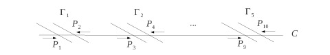
It will be convenient to re-index the relative points as where and . We will construct a relative marked ruled surface such that:
-
•
The special fiber is simply .
-
•
The special section ; here is a horizontal section of and is the fiber of above , for each .
-
•
The relative points on are such that on , for general .
-
•
Each limit point is a general point on the fiber .
The construction generalizes the case of eleven points. Namely, we first choose relative points in specializing to in a general way. Next, let and . It follows that
Consider the short exact sequence on :
(Note that , so the sequence is unique). By Prop. 6.4, the sequence can be extended to
over , where is locally free. Finally, we take and . It follows that . We take to be the strict transform of the on the blowup at .
Next, we will distinguish between two cases: and .
13.3. Semistability
Let be the horizontal section of through . Just as in the case of eleven points, we can show that the conormal bundle is semistable of slope 1/2.
13.4. Second Degeneration
In this case, we perform another degeneration on the trivial ruled surface . Fix general horizontal sections of . Let for and . Next, we specialize the relative points to by “sliding” them along the corresponding fibers , in a general way.
13.5. Semistability
Denote by the blowup of at the relative points constructed in the previous step. Now, is obtained from by applying elementary transforms at general points on the fixed fibers through . Since , it follows that the resulting vector bundle is semistable of slope (the proof is similar to that of Lemma 3.2).
13.6. Invariants
The computation of invariants was carried out in Section 7. This completes the proof of the Main Theorem.
Appendix A The Indecomposable Elliptic Ruled Surface of Degree 1
Below we summarize some facts about the indecomposable elliptic ruled surface of degree 1. Our references are [2] and ([8], Chapter V.2).
Let be an elliptic curve. Let be an indecomposable rank 2 vector bundle of degree 1 on . Then, arises as the unique nontrivial extension
| (1) |
where .
Let us compute the symmetric powers of . By ([2], Lemma 22 on p.439), we have:
where the are the nontrivial line bundles with . Also, by ([2], Cor. to Thm. 7 on p.434), we have and . Finally, we have the Clebsch-Gordan formula ([2], p.438) for a rank 2 vector bundle:
Using the above, we find:
In general, if is even, decomposes as a sum of line bundles that are isomorphic to or . If is odd, decomposes as a sum of copies of .
Next, consider the ruled surface together with the projection . We identify with the unique section of . The anticanonical class of is
Note that
We have:
Proposition A.1.
Let be the indecomposable vector bundle of rank 2 and degree 1, . Consider the ruled surface .
-
(a)
For any , there is a unique curve on .
-
(b)
There are precisely 3 curves , , on that are numerically equivalent to . Their rational equivalence classes are given by for each nontrivial line bundle with .
-
(c)
The linear system sweeps a base-point free pencil on . There are 3 nonreduced sections, namely , . Any other section is a smooth elliptic curve isomorphic to (the natural projection being the usual multiplication-by-2 map).
Proof.
a) This follows from the fact that is the unique indecomposable rank 2 vector bundle with determinant .
b) This follows from
c) We have Therefore , i.e. sweeps a pencil on . Next, let any section of other than , . From part b), is irreducible. Since is of arithmetic genus 1, it follows that is a smooth elliptic curve. One can show that is isomorphic to as follows. First, one shows that every irreducible section of is isomorphic to the fixed section . Next, one checks that, for any , admits a 2:1 cover to . It follows that is the isogeny dual to . ∎
Appendix B Some Continued Fractions
Let where and . Consider the matrix
For any positive integer , define
Note that and .
For example,
and
The ratios and have natural expansions as continued fractions approximating (the later are palindromic). In particular,
are precisely the constants in Theorem 4.1 and the Main Theorem.
Lemma B.1.
Let and be any real numbers.
-
(a)
The following are equivalent:
-
(b)
The following are equivalent:
Proof.
(a) Multiply both sides by and substitute :
(b) Multiply both sides by and substitute :
∎
References
- [1]
- [2] M. Atiyah, Vector bundles over an elliptic curve, Proc. Lond. Math. Soc. (3) 7 (1957), 414–452.
- [3] C. Ciliberto, O. Dumitrescu, R. Miranda, J. Roé, Emptiness of homogeneous linear systems with ten general base points, “Classification of Algebraic Varieties,” EMS Series of Congress Reports (2011), 189–195.
- [4] C. Ciliberto, R. Miranda, Homogeneous interpolation on ten points, J. Algebraic Geom. 20 (2011), no. 4, 685–726.
- [5] C. Ciliberto, R. Miranda, Linear systems of plane curves with base points of equal multiplicity, Trans. Amer. Math. Soc. 352 (2000), no. 9, 4037–4050.
- [6] T. Eckl, Ciliberto-Miranda degenerations of blown up in 10 points, J. Pure Appl. Algebra 215 (2011), no. 4, 672–696.
- [7] R. Friedman, “Algebraic Surfaces and Holomorphic Vector bundles,” Springer, 1998.
- [8] R. Hartshorne, “Algebraic Geometry,” Springer, 1977.
- [9] M. Maruyama, Openness of a family of torsion free sheaves, J. Math. Kyoto Univ. 16 (1976), no. 3, 627–637.
- [10] M. Nagata, On the fourteenth problem of Hilbert, Amer. J. Math. 81 (1959), 766–772.
- [11] I. Petrakiev, Multiple points in and degenerations to elliptic curves, Proc. Amer. Math. Soc. 137 (2009), no. 1, 65–71.
- [12] J. Le Potier, “Lectures on Vector Bundles,” Cambridge Univ. Press (1997).