Statistical modelling of higher-order correlations in pools of neural activity

Abstract

Simultaneous recordings from multiple neural units allow us to investigate the activity of very large neural ensembles. To understand how large ensembles of neurons process sensory information, it is necessary to develop suitable statistical models to describe the response variability of the recorded spike trains. Using the information geometry framework, it is possible to estimate higher-order correlations by assigning one interaction parameter to each degree of correlation, leading to a $(2^{N}-1)$-dimensional model for a population with $N$ neurons. However, this model suffers greatly from a combinatorial explosion, and the number of parameters to be estimated from the available sample size constitutes the main intractability reason of this approach. To quantify the extent of higher than pairwise spike correlations in pools of multiunit activity, we use an information-geometric approach within the framework of the extended central limit theorem considering all possible contributions from high-order spike correlations. The identification of a deformation parameter allows us to provide a statistical characterisation of the amount of high-order correlations in the case of a very large neural ensemble, significantly reducing the number of parameters, avoiding the sampling problem, and inferring the underlying dynamical properties of the network within pools of multiunit neural activity.

• Extended Central Limit Theorem; Large neural ensemble; Multiunit neural activity; Information Geometry
  PACS: 02.50.-r; 05.45. Tp;87.19.La.

1 Introduction

To understand how sensory information is processed in the brain, we need to investigate how information is represented collectively by the activity of a population of neurons. There is a large body of evidence suggesting that pairwise correlations are important for information representation or processing in retina [1, 2], thalamus [3] and cerebral [4, 5, 6] and cerebellar cortices [7, 8]. However, there is also evidence that in at least some circumstances, pairwise correlations do not by themselves account for multineuronal firing patterns [9, 10]; in such circumstances, triplet and higher-order interactions are important. The role of such higher-order interactions in information processing is still to be determined, although they are often interpreted as a signature of the formation of Hebbian cell assemblies [11].

Higher-order correlations may be important for neural coding even if they arise from random fluctuations. Amari and colleagues [12] have suggested that a widespread distribution of neuronal activity can generate high-order stochastic interactions. In this case, pairwise or even triplet-wise correlations do not uniquely determine synchronised spiking in a population of neurons, and high-order interactions across neurons cannot be disregarded. Thus, to gain a better understanding of how neural information is processed, we need to study, whether higher-order interactions arise from cell assemblies or from stochastic fluctuations. Information-geometric measures can be used to analyse neural firing patterns including correlations of all orders across the population of neurons [13, 14, 15, 16, 17, 18, 9, 10].

A straightforward way to investigate the neural activity of a large population of neurons is to use binary maximum entropy models incorporating pairwise correlations on short time scales [1, 2]. To estimate this model, one has to consider a sufficient amount of data to measure the mean activity of individual neurons and correlations in pairs of neurons. This allows us to estimate the functional connectivity in a population of neurons at pairwise level. However, if higher-order correlations are present in the data, and as the number of possible binary patterns grows exponentially with the number of neurons, we would need to use an appropriate mathematical approach to go beyond a pairwise modelling. This is in general a difficult problem, as sampling even third-order interactions can be difficult in a real neurophysiological setting [9, 10].

However, under particular constraints, this sampling difficulty can be substantially ameliorated. An example of such a constraint is pooling, in which the identity of which neuron fires a spike in each pool is disregarded. Such a pooling process reflects the behaviour of a simple integrate-and-fire neuron model in reading out the activity of an ensemble of neurons. It also reflects a common measurement made in systems neuroscience: the recording of multiunit neural activity, without spike sorting. Whether or not such constraints permit a complete description of neural information processing is still a matter of debate [6, 10], but they may allow substantial insight to be gained into the mechanisms of information processing in neural circuits. A method for the statistical quantification of correlations higher than two, in the representation of information by a neuronal pool, would be extremely useful, as it would allow the degree of higher - order correlations to be estimated from recordings of multiunit activity (MUA) - which can be performed in a much broader range of circumstances than “spike-sortable” recordings can.

In this paper, we use a pooling assumption to investigate the limit of a very large neural ensemble, within the framework of information geometry [12, 13, 14, 15, 16, 17, 18, 19, 20]. In particular, we take advantage of the recent mathematical developments in $q$-geometry (and $q$-information geometry) and the extended central limit theorem [21, 22, 23, 24, 25, 26] to provide a statistical quantification of higher-order spike correlations. This approach allows us to identify a deformation parameter to characterise the extent of spike correlations higher than two in the limit of a very large neuronal ensemble. Our method accounts for the different regimes of firing within the probability distribution and provides a phenomenological description of the data, inferring the underlying role of noise correlations within pools of multiunit neural activity.

2 Methodology

2.1 Information geometry and the pooled model

We represent neuronal firing in a population of size $N$ by a binary vector $X=(x_{1},\ldots,x_{N})$, where $x_{i}=0$ if neuron $i$ is silent in some time window $\Delta T$ and $x_{i}=1$ if it is firing (see Fig 1a). Then, for a given time window, we consider the probability distribution of binary vectors, $\{P(X)\}$. Any such probability distribution $\{P(X)\}$ is made up of $2^{N}$ probabilities

$$P(X)=Prob\{X_{1}=i_{1},...,X_{N}=i_{N}\}=P_{i_{1}...i_{N}}$$ (1)

subject to the normalization

$$\sum_{i_{1},...,i_{N}=0,1}P_{i_{1}...i_{N}}=1.$$ (2)

As proposed by Amari and co-workers (see, for instance, Refs [20, 15]), the set of all the probability distributions $\{P(X)\}$ forms a ($2^{N}-1$)-dimensional manifold ${S_{N}}$. This approach uses the orthogonality of the natural and expectation parameters in the exponential family of distributions. It is also useful for analysing neural firing in a systematic manner based on information geometry. Any such probability distribution can be unequivocally determined using a coordinate system. One possible coordinate system is given by the set of $2^{N}-1$ marginal probability values:

$$\tilde{\eta}_{i}=E[x_{i}]=P\{x_{i}=1\}, i=1,...,N$$ (3)

$$\tilde{\eta}_{ij}=E[x_{i}x_{j}]=P\{x_{i}=x_{j}=1\}, i<j$$ (4)

$$\vdots$$

$$\tilde{\eta}_{123...N}=E[x_{1}...x_{N}]=P\{x_{1}=x_{2}=...=x_{N}=1\}.$$ (5)

These are called the $\tilde{\eta}$-coordinates [20]. Moreover, provided $P(X)\neq 0$, any such distribution can be expanded as in Ref. [15]

$$P(X)=\exp\left\{\sum_{i=1}^{N}{x_{i}}\tilde{\theta}_{i}+\sum\limits_{i<j}{x_{i}}x_{j}\tilde{\theta}_{ij}+\right.$$

$$\left.+\sum\limits_{i<j<k}{x_{i}}x_{j}x_{k}\tilde{\theta}_{ijk}+\ldots+x_{1}\ldots x_{N}\tilde{\theta}_{1\ldots N}-\tilde{\psi}\right\},$$

where there are in total $2^{N}-1$ different $\tilde{\theta}$ correlation coefficients that can be used to determine univocally the probability distribution. The $\tilde{\theta}$ forms a coordinate system, named $\tilde{\theta}-coordinates$, which correspond to e-flat structure in the $(2^{N}-1)$-dimensional manifold $S_{N}$. In Eq. (2.1), $\tilde{\psi}$ is a normalization term. The $\tilde{\eta}$-coordinates and $\tilde{\theta}$ coordinates are dually orthogonal coordinates. The properties of the dual orthogonal coordinates allow the formulation of the generalised Pythagoras theorem that gives a decomposition of the Kullback Leibler divergence to calculate contributions of different orders of interaction between two probability distributions.

These notions are rigorously developed in Refs. [12, 14, 15, 16, 17, 18, 19, 20] within the framework of information geometry. Assigning one “interaction parameter” $\tilde{\theta}$ to each degree of correlation, we have a ($2^{N}-1$)-dimensional model for a population with $N$ neurons. The basis of this formalism is shown in Fig 1b: once our coordinate $\tilde{\theta}$ is fixed we have a subset $E(\tilde{\theta})$ for each possible value of $\tilde{\theta}$ and an exponential family of distributions (with the same value of $\tilde{\theta}$). Notice that when higher-order correlations are considered, we need to construct an orthogonal multidimensional coordinate space to build the probability distribution, as is schematised in Fig 1b. Let us consider $M(\tilde{\eta}_{1},...,\tilde{\eta}_{N})$ to be a submanifold of the marginals in $S_{N}$. Then, the tangential direction of $M(\tilde{\eta}_{1},...,\tilde{\eta}_{N})$ represents the direction in which only the pure correlation changes, while the tangential directions of $E(\tilde{\theta})$ span the directions in which only $\tilde{\eta}_{1},...,\tilde{\eta}_{N}$ change but $\tilde{\theta}$ is fixed. Directions of changes in the correlations and marginals are required to be mutually orthogonal.

It is important to point out that the estimation of all the parameters associated with higher-order correlations suffers greatly from a combinatorial explosion. Consider, for instance, a population of 50 neurons for which we would need therefore more than $10^{15}$ parameters. Thus, the number of parameters to be estimated from the available sample size constitutes the reason for the intractability of this approach.

However, if we assume that a neuron cannot process spikes from different neurons separately, then the labels of the neurons that fired each of the spikes are lost. In this case, the target neuron is only aware of the number of synchronous firings among its inputs. Similarly, a neurophysiological recording technique that disregards the identity of the neuron that fires each spike (i.e. it measures MUA) can only count the number of cells in the vicinity firing in a time window, rather than provide information about their pattern.

To investigate the effects of such processes, we consider a pooled model [13, 12], where we assume (for mathematical convenience) a population of $N$ identical neurons. Rather than the full distribution of $X$ with probabilities $P(X)$ considered above, we now introduce a set of probabilities $P(k)$ where $k=0,1,\ldots,N$ represents the number of synchronous spiking neurons in the population during a time interval $\Delta T$.

This assumption greatly simplifies the analysis based on the coordinate systems described above. The probability distribution is now characterised by only $N$ parameters. Following Ref. [9], we refer to the probability values $P(k)$ as the $p$-coordinates (the pooled model is defined by $N$ parameters). Then, considering the number of neurons that are firing simultaneously (within $\Delta T$) in the pooled model, instead of the probability distribution Eq. (2.1), one has

$$P(1)=N\exp{\left(\theta_{1}-\psi(\theta)\right)},\\$$ (7)

and

$$P(k)=\binom{N}{k}\,\exp{\left(k\ \theta_{1}+\sum\limits_{i=2}^{k}\binom{k}{i}\ \theta_{i}-\psi(\theta)\right)}, k=2,\ldots,N$$ (8)

while $P(0)=\exp(-\psi(\theta))$ corresponds to a completely silent response and is written in such way so as to fulfil normalization of the probabilities $\{P(k)\}$. The marginals $\eta_{k}$, indicating the probability of any $k$ neurons firing within $\Delta T$, are given by $\eta_{k}=\sum\limits_{i=k}^{N}\binom{N-k}{i-k}\frac{P(i)}{\binom{N}{i}},$ with $k=0,1,\ldots,N$ [13]. In Eqs. (7) and (8), $\theta_{1}$ corresponds to the first order contribution to the log probabilities, while each $\theta_{i}$ ($i=2,\ldots,N$) represents the effect on the log probabilities of interactions of order $i$ in the neuronal pool. We will deal with the relative probability of simultaneous spiking. The ratio between $P(k)$ and $P(k-1)$ is given by the following expressions:

$$\frac{{P(1)}}{{P(0)}}=N\exp(\theta_{1}),$$ (9)

$$\frac{{P(2)}}{{P(1)}}=\frac{N-1}{2}\exp(\theta_{1}+\theta_{2}),$$ (10)

and if $k>2$

$$\frac{{P(k)}}{{P(k-1)}}=\frac{{N-k+1}}{k}\,\exp\left({\theta_{1}+\sum\limits_{i=2}^{k-1}{\frac{{(k-1)!}}{{(i-1)!(k-i)!}}}\ \theta_{i}+\theta_{k}}\right).$$ (11)

This approach has been applied in a previous publication [9] within the maximum entropy (ME) principle to evaluate whether high-order interactions play a role in shaping the dynamics of neural networks. By fixing the correlation coordinate $\theta_{k+1}=0$ in Amari’s formalism, the ME constraints are set up to order $k$. This is, the ME principle is archived by simple fixing $\{\theta_{i}\}_{i>k}=0$ and the distribution is determined by $\{\theta_{i}\}_{i\leq k}$. The constraints of the ME principle allow us to choose the most random distribution subject to these constraints [15, 9]. Thus correlation structures that do not belong to the constrained features are simply removed. Let us consider for instance ME constraints at pairwise level that are set by fixing $\{\theta_{i}\}_{i>2}=0$, therefore all correlation structures of order higher than two are removed.

In a recent paper, Yu et al [27] have shown that higher - order correlation structures are quite crucial to get a better understanding of how information might be transmitted in the brain. They have reported the importance of higher - order interactions to characterise the cortical activity and the dynamics of neural avalanches, exhaustively analysing how the Ising like models [28, 1, 2, 29] do not provide in general a fair description of the overall organization of neural interactions when considering large neuronal systems.

2.2 A simple binomial approach

In order to get a better understanding of how to take the limit of a very large number of neurons, we first discuss a quite naive approach using Bernoulli trials and a binomial distribution. Despite its simplicity and limitations, it helps to provide some intuitive feedback.

Let us consider the activity of a neuronal population of $N$ neurons in a specific time window $\Delta T$. It should be noted that $P(k)$ denotes the probability of $k$ cells firing simultaneously and $N-k$ being silent, with $0\leq k\leq N$. Let us denote by $\lambda$ the mean number of spiking cells, then $\lambda=E_{P}[k]=\sum_{k=0}^{N}kP(k)\equiv N\,p$ where we introduced $p=\frac{\lambda}{N}$.

If we assume that members of a population of neurons spike independently and with a fixed, constant probability, then the spiking activity of the population can be modelled as Bernoulli trials. For a population containing $N$ neurons, each with a firing probability $p$, the probability $P(k)$ of having $k$ neurons firing simultaneously is given by the binomial distribution: $P(k)=b(k;N,p)=\binom{N}{k}p^{k}(1-p)^{N-k},$ with $k=0,1,\ldots,N$. In the limit of large $N$ and small $p$, such that $\lambda=Np$ is finite, one has the so-called Poisson regime [30]. In this case, the following relations hold for $k\geq 1$:

$$\frac{{b(k;N,p)}}{{b(k-1;N,p)}}=\frac{\lambda}{k}+O(\frac{1}{N}),$$ (12)

in the particular case $k=1$ we have

$$\frac{{b(1;N,p)}}{{b(0;N,p)}}=\lambda+O(\frac{1}{N}),$$ (13)

while for $k=0$ the distribution in the Poisson regime reads

$${{b(0;N,p)}}=\exp{(-\lambda)}+O(\frac{1}{N}).$$ (14)

We now introduce these ansätze in Eqs. (9)-(11). The ratio between the distribution one would derive in the absence of knowledge of spike correlation, $P(1)$, and the distribution one would obtain when no spike is being fired, $P(0)$, is given by $\frac{P(1)}{P(0)}=Ne^{\theta_{1}}.$ Let us consider the limit $N\to\infty$ with $\lambda=N\,p$ finite ($p$ is a small quantity). Then, comparing Eq. (13) with Eq. (9), we can write $\lambda=Ne^{\theta_{1}}+O(\frac{1}{N}),$ which leads to

$$\theta_{1} \approx \ln\left(\frac{\lambda}{N}\right).$$ (15)

Notice that in this regime, using Eq. (14), the probability distribution $P(k)$ at $k=0$ behaves as ${\rm{\emph{P(0)}}}\equiv e^{-\psi}=e^{-\lambda}+O(\frac{1}{N})$, which gives $\psi$ approximately equal to $\lambda$ for the normalizing factor.

Introducing Eq. (15) into the probability of $k$ neurons firing, Eq.(8), as
$\mathop{\lim}\limits_{N\to\infty}\frac{{N(N-1)\ldots(N-(k+1))}}{{(N)^{k}}}=1$, in the large $N$ limit, we get $P(k,\lambda)\approx\frac{{\lambda^{k}}}{{k!}}e^{-\psi(\theta)}e^{\ {\sum\limits_{i=2}^{k}{\binom{k}{i}}\theta_{i}}}.$ Summing up, if a neuronal population behaves in the large $N$ limit such that

$$\psi(\theta)\approx\lambda$$ (16)

and accomplishes Eq. (15) then the probability of $k$ cells firing simultaneously can be expressed as a $\tilde{\delta}$-deformed Poisson distribution such as:

$$P_{\tilde{\delta}}(k,\lambda)\approx\frac{\lambda^{k}e^{-\lambda}e^{\tilde{\delta}(k)}}{k!},$$ (17)

where $\tilde{\delta}(k)\equiv{\sum\limits_{i=2}^{k}\binom{k}{i}\theta_{i}}$ is a deformation term that summarises correlations of all orders.

Eq. (17) corresponds to a Poisson distribution modulated by a multiple-correlation : $e^{\tilde{\delta}(k)}$. Notice that in the analytical approach presented above we have taken the limit of $N\rightarrow\infty$, but if only correlations up to order two dominated the neuronal spiking, the departure from a Poissonian behaviour in the probability of $k$ ($\geq 2$) firing neurons would be small. Indeed, applying Amari’s prescription [12], we obtain $\tilde{\delta}(2)=\theta_{2}=O(\frac{1}{N})$ and then $e^{\tilde{\delta}(k)}$ is almost unity. But our derivation comprises all orders through the factor $e^{\tilde{\delta}(k)}$.

It is important to note that we consider the mean number of spiking cells to be equal to the normalization factor (see Eq. (16)). This assumption represents only a possible subset of the probability distributions $\{P(X)\}$ presented in Eq. (2.1). Thus, in the limit of a very large number of neurons, and if higher - orders are taken into account, we cannot provide an analytical estimate of the entire set of all possible widespread distributions using the approach of Eq. (17).

More importantly, due to the high dimensionality involved in determining Eq. (2.1), or even in our approach of Eq. (17), we have to take just a few correlation terms to avoid having an intractable number of parameters [14, 9].

But the more basic limitation of the above approach is due to the fact that taking a limit of a very large number of neurons or “thermodynamic limit” essentially means to account for the central limit theorem of statistics (CLT). The CLT articulates conditions under which the mean of a sufficiently large number of independent random variables, each with finite mean and variance, can be considered as normally distributed [31]. In the next sections we discuss how to take the limit of a very large number of neurons accounting also for higher-order correlations in the probability distribution. Importantly, we consider the case of any probability distribution of firing, and do not just simply model the neural activity through a binomial distribution (or Bernoulli trials). We make use of an extension of the central limit theorem that also accounts for the case of correlated random variables [24]. This is particularly important since it allows us to extend analytical models accounting for effect the of high - order correlations on the PDFs, making it possible to compute the emergent properties of the system in the “thermodynamic limit”.

2.3 $q$-Information geometry

Recent studies on information geometry and complex systems have found a big number of distributions that in the asymptotic limit obey the power law rather than the Gibbs distribution [20, 32, 12, 23, 33]. These power law distributions seem to rule the asymptotic regime, and the $q$-exponential distributions used in non-extensive statistical mechanics are very useful for capturing such phenomena [32, 24, 22, 23, 25, 26, 20, 21]. The geometrical structure of such probability distributions is termed $q$-geometry, and its mathematical foundations have been developed by Tsallis, Gell-Mann, Amari, and collaborators. They have in particular proved that the $q$-geometrical structure is very important to investigate systems with weakly and strongly correlated random variables [32, 24, 22, 23, 25, 26, 20, 21].

In particular, recently Amari and Ohara [21] proved that it is possible to generalise the $q$-structure to any family of probability of distributions, and that the family of $q$-structure is ubiquitous since the of family of all probability distributions can always be endowed with the structure of the $q$-exponential family for an arbitrary $q$.

The $q$-exponential is defined as

$$\exp_{q}(x)=\begin{cases}[1+(1-q)(x)]^{\frac{1}{1-q}}&\text{if $(1+(1-q)(x))>0$;}\\ 0&\text{otherwise}\end{cases}$$ (18)

where the limiting case of $q\rightarrow 1$ reduces to $\exp_{1}(x)=\exp(x)$. The $q$-exponential family is defined by generalising Eq. (2.1) (for a review see [21]) as

$$P_{q}(x,\Theta)=\exp_{q}\{\Theta\cdot x-\psi(\Theta)\},$$ (19)

where in particular the $q$-Gaussian distribution is defined as $p(x,\mu,\sigma)=\exp_{q}(-\frac{(x-\mu)^{2}}{2\sigma^{2}}-\psi(\mu,\sigma))$ (see Appendix, Section B, for a connection with the correlation coordinates).

In analogy with the exponential families the $q$-geometry has a dually flat geometrical structure (as its coordinates are orthogonal) and accomplishes the $q$-Pythagorean theorem. The maximiser of the $q$-escort distribution is a Bayesian MAP (maximum a posteriori probability) estimator as proved in Ref. [21]. Moreover, it is possible to generalise the $q$-structure to any family of probability distributions, because any parameterised family of probability distributions forms a submanifold embedded in the entire manifold. Altogether, we can introduce the $q$-geometrical structure to any arbitrary family of probability distributions and guarantee that the family of all the probability distributions belongs to the $q$-exponential family of distributions for any $q$ [21]. We refer to Fig 2 for a schematic explanation of the $q$-exponential family.

Next, we take advantage of recent mathematical progress on $q$-geometry (and $q$-information geometry) to investigate the effect of high - order correlations on the probability distribution in the asymptotic limit.

3 Results

3.0.1 Beyond pairwise correlations

In statistical mechanics it is said that we reach the “thermodynamic limit” when the number of particles being considered reaches the limit $N\rightarrow\infty$. The thermodynamic limit is asymptotically approximated in statistical mechanics using the so-called central limit theorem (CLT) [31]. The CLT ensures that the probability distribution function of any measurable quantity is a normal Gaussian distribution, provided that a sufficiently large number of independent random variables with exactly the same mean and variance are being considered (see pages 324-330 [31]). Thus, the CLT does not hold if correlations between random variables cannot be neglected.

Thus, the CLT articulates conditions under which a sufficiently large number of independent and identically distributed random variables, each with finite mean and variance, can be considered as normally distributed [31]. In particular, the CLT has been used by Amari and colleagues [12] to estimate the joint probability distribution of firing in a neuronal pool considering the limit of a very large number of neurons. Thus, in their approach pairwise correlations within the joint distribution of firing are quantified through the covariance $<U_{i}U_{j}>$ of the weighted sum of inputs $U_{i}$ and $U_{j}$ of two given pairs of neurons ($i\neq j$, $i=1...N$ and $j=1...N$ ) [12]. This is $U_{i}=\sum_{j=1}^{m}w_{ij}-H$, where $w_{ij}$ is the connection weight from the $j^{th}$ input to the $i^{th}$ neuron ($H=E[U_{i}]$ denotes the mean). Importantly, these $U_{i}$ are being considered Gaussian due to the CLT [12], and thus the approach quantifies the amount of pairwise correlations through the covariance $<U_{i}U_{j}>$.

In the presence of weak or strong correlations of any sort, the CLT has been generalised in recent publications by M Gell-Mann, C Tsallis, S Umarov, C Vignat, A Plastino (see:[22, 23, 24, 25, 26]). They have proved that when a system with weakly or strongly correlated random variables is being considered, if we gather a sufficiently large number of such systems together, the probability distribution will converge to a $q$-Gaussian distribution [22, 23, 24, 25, 26]. This is in agreement with the theorems recently proved by Amari and Ohara [21], which permit the introduction of the $q$-geometrical structure to any arbitrary family of probability distributions, and guarantee that the family of all the probability distributions belongs to the $q$-exponential family of distributions.

We will use the “natural extension” of the central limit theorem (ECLT) proposed in [24], which accounts for cases in which correlations between random variables are non-negligible. This results in so-called $q$-Gaussians (instead of Gaussians) as the PDFs in the ECLT, as proved in Ref.[24]:

$$G_{q}(x)=\begin{cases}[1+\frac{(1-q)(-x^{2})}{2}]^{\frac{1}{1-q}}&\text{if $(1+\frac{(1-q)(-x^{2})}{2})>0$,}\\ 0&\text{otherwise}\end{cases}$$ (20)

where $q$ is a (problem-dependent) positive real index. Notice that in the limit of $q=1$ a normal Gaussian distribution is recovered as $\lim_{N->\infty}(1+\frac{1}{N})^{N}=e,$ which can be rephrased as $\lim_{q->1}(1+(1-q))^{\frac{1}{(1-q)}}=e$. In other words, the CLT is being recovered as $q\rightarrow 1$ [22, 23, 24, 25, 26].

Let us now consider the probability of exactly $k=N\cdot r$ (and thus $r=\frac{k}{N}$) neurons firing within a given time window $\Delta T$ across a population of $N$ neurons. In the framework of the pooled model we have:
$P_{r}[r=\frac{k}{N}]=P_{r}\{x_{1}=x_{2}=\ldots=x_{k}=1,x_{k+1}=\ldots=x_{N}=0\},$ where the neuron $x_{i}$ is subject to a weighted sum of inputs $u_{i}$, thus $x_{i}=1$ if and only if $u_{i}>0$ and $x_{i}=0$ if $u_{i}\leq 0$. Following [12], the neuronal pool receives common inputs $s_{1},s_{2},...s_{M}$ (as schematised in Fig 3), and $u_{i}$ is weighted by the common inputs $u_{i}=\sum_{j=1}^{M}w_{ij}s_{j}-h$, where $w_{ij}$ are randomly assigned connections weights. These $u_{i}$ are $q$-Gaussian due of the ECLT [22, 23, 24, 25, 26]. Considering that the $u_{i}$ are subject to a $q$-Gaussian distribution $N_{q}(-h,1)$, we define in analogy to [12] $u_{i}=\sqrt{1-\alpha}\,v_{i}+\sqrt{\alpha}\,\varepsilon-h$, for $i=1,..,N$. We take $\alpha=E_{q}[u_{i}u_{j}]$ as a $q$-variance, $h=E_{q}[u_{i}]$ as the $q$-mean, and two independent $q$-Gaussian random variables $v_{i}$ and $\varepsilon$ subject to $N_{q}(0,1)$ (see [34] for a detailed description of $q$-Gaussian random variables).

In the following we will use what is commonly referred to factorization approach in statistical mechanics [35, 36], which is applicable in this case as we are considering weak correlations among neurons and the population of neurons is homogenous. We name $E_{\varepsilon}$ as the expectation value taken with respect to a random variable $\varepsilon$, and $P_{r}\{u>0|\varepsilon\}$ is the conditional probability for $\varepsilon$. This allows us to calculate the probability of having $r=\frac{k}{N}$ neurons firing, separating the contribution of neurons that are firing $[P_{r}\{u>0|\varepsilon\}]^{k}$ from those that are silent $[P_{r}\{u\leq 0|\varepsilon\}]^{N-k}]$, as

$$\begin{split}P_{r}\{x_{1}=x_{2}=\ldots=x_{k}=1,x_{k+1}=\ldots=x_{N}=0\}=\\ E_{\varepsilon}[P_{r}\{u_{1};u_{2};\ldots;u_{k}>0,u_{k+1};\ldots;u_{N}\leq 0|\varepsilon\}]\equiv\\ E_{\varepsilon}[(\begin{array}[]{c}N\\ k\end{array})[P_{r}(u>0|\varepsilon)]^{k}[P_{r}(u\leq 0|\varepsilon)]^{N-k}].\\ \end{split}$$ (21)

In order to go beyond the pairwise estimation of [12] (performed within the CLT framework), we need to quantify the amount of correlations higher than two in the probability distributions. If we take the limit of $N\rightarrow\infty$, in the framework of the $q$-Gaussian ECLT [22, 23, 24, 25, 26], instead of the Gaussian CLT as considered in [12], we can define:

$${F_{q}(\varepsilon)}\equiv P_{r}(u>0|\varepsilon) = P_{r}(u_{i}>\frac{h-\sqrt{\alpha}\varepsilon}{\sqrt{1-\alpha}})$$

$$= \frac{1}{\sqrt{2\pi}}\int_{\frac{h-\sqrt{\alpha}\varepsilon}{\sqrt{1-\alpha}}}^{\infty}\!\exp_{q}{(-\frac{v^{2}}{2})}\,dv.$$

If we take $q=1$ in the probability of having $r=\frac{k}{N}$ neurons firing in Eq. (3.0.1), and the distributions within the integral of Eq. (3.0.1) corresponds to normal Gaussian distributions, and we are in the “CLT framework”. On the other hand, the “ECLT framework” corresponds to $q>1$ and in this case the system has weakly or strongly correlated random variables. Thus the distributions within the integral of Eq. (3.0.1) are considered as q-Gaussian distributions, and correlations are quantified through $q$.

Notice that if we consider the limit of the CLT framework ($q=1$), the previous expression reduces to

$${F_{q=1}(\varepsilon)}=\frac{1}{2}\mathrm{Erfc}(\frac{1}{\sqrt{2}}\frac{h-\sqrt{\alpha}\varepsilon}{\sqrt{1-\alpha}})$$ (23)

where $\mathrm{Erfc(x)}=\frac{2}{\sqrt{\pi}}\int_{x}^{\infty}\exp(-t^{2})dt$ denotes the complementary error function. However, if the effect of correlations higher than two is not negligible then according to the ECLT: $q>1$, thus

$$\exp_{q}(-\frac{v^{2}}{2})=\frac{1}{\Gamma(\frac{1}{q-1})}\int_{0}^{\infty}dt\,t^{\frac{1}{q-1}-1}\exp({-t-t(q-1)\frac{v^{2}}{2}}),$$ (24)

which is known as Hilhorst transform [37], an integral representation widely used in generalised statistical mechanics [38]. Thus $F_{q}(\varepsilon)$ reads

$$\begin{split}{F_{q}(\varepsilon)}=\frac{1}{\Gamma(\frac{1}{q-1})}\int_{0}^{\infty}\int_{\frac{h-\sqrt{\alpha}\varepsilon}{\sqrt{1-\alpha}}}^{\infty}dt\,dv\,t^{\frac{1}{q-1}-1}\exp({-t+t(q-1)\frac{v^{2}}{2}}).\end{split}$$ (25)

Using several non-trivial identities between Gauss hypergeometric functions and the incomplete beta function, we can exactly calculate the integrals expressed above (see Appendix Section A, for a detailed description of the math). And ${F_{q}(\varepsilon)}$ in terms of a beta incomplete function reads

$$\begin{split}{F_{q}(\varepsilon)}=\frac{1}{{2\sqrt{2\pi}}\sqrt{\frac{q-1}{2}}}{B_{\frac{1}{1+\xi_{0}(\varepsilon)}}(\frac{1}{q-1},\frac{1}{2})},\end{split}$$ (26)

where

$$\xi_{0}(\varepsilon)=\frac{(q-1)(h-\sqrt{\alpha}\varepsilon)^{2}}{2({1-\alpha})}.$$ (27)

Eq.( 26) allows us to calculate the probability (Eq. LABEL:prprob) of exactly $k$ neurons firing within a given time window $\Delta T$ across a population of $N$ neurons. Notice that the amount of correlations higher than two is quantified through $q>1$, as when $q$ is constrained to 1 it leads to ${F_{q=1}(\varepsilon)}$, which is reduced to the estimation within the CLT (Eq. 23) as in [12].

The joint distribution of firing can therefore be estimated as

$$Q_{q}(r) \simeq NP_{r}[r=\frac{k}{N}]$$ (28)

$$= NE_{\varepsilon}\{\left(\begin{array}[]{c}N\\ k\end{array}\right)[{F_{q}(\varepsilon)}]^{k}[1-F_{q}(\varepsilon)]^{N-k}\}.$$ (31)

The expectation value $E_{\varepsilon}$ can be estimated using the saddle point approximation [39, 12]

$$\begin{split}Q_{q}(r)=\sqrt{\frac{1}{r(1-r)|z_{q}^{\prime\prime}(\varepsilon_{0})|}}\frac{1}{\sqrt{2\pi}}\exp[Nz_{q}(\varepsilon_{0})-\frac{{\varepsilon_{0}}^{2}}{2}],\end{split}$$ (32)

where $z_{q}(\varepsilon)=r\log(\frac{{F_{q}(\varepsilon)}}{r})+(1-r)\log(\frac{1-{F_{q}(\varepsilon)}_{q}}{1-r})$. Within the saddle point approximation: $\varepsilon_{0}=\mathrm{\arg\max_{\varepsilon\epsilon\mathbb{R}}}\left[z_{q}(\varepsilon)\right]$ and $\frac{dz(\varepsilon)}{d\varepsilon}=0$. The solution is $\varepsilon_{0}={F_{q}^{-1}(r)},$ which implies $r={F_{q}(\varepsilon_{0})},$ where $r$ goes between $[0,1]$ and $\varepsilon_{0}$ is defined for all real numbers. $\xi_{0}(\varepsilon)$ (Eq. 27) can take different values with $\alpha$ and $h$. Additionally, $\varepsilon_{0}={F_{q}^{-1}(r)}$ depends on the degree of correlation of the network architecture, which is quantified by $q$. Fig 4 shows the behaviour of $Q_{q}(r)$ for $q=1.3$ in comparison to $q=1$. Notice that a higher degree of correlation, $q>1$, corresponds to a more widespread distribution. This is in agreement with the idea of Amari and Nakahara [12] that when taking a very large number of neurons higher-order correlations are needed to reproduce the behaviour of a widespread distribution.

Estimating Eq. (32) for $q>1$ requires a non trivial approach: finding $\varepsilon_{0}={F_{q}^{-1}(r)}$, and from Eq. (26) this means to estimate the inverse incomplete beta function of ${B_{\frac{1}{1+\xi_{0}(\varepsilon)}}(\frac{1}{q-1},\frac{1}{2})}$ (multiplied by the factor $\frac{1}{{2\sqrt{2\pi}}\sqrt{\frac{q-1}{2}}}$). The inverse beta functions are tabulated in exhaustive detail, thus we can perform the numerical estimation of Eq. (32). It is important to note that the incomplete beta function subroutines in matlab are normalised as ${I_{w}(p,s)}=\frac{\int_{0}^{w}t^{s-1}(1-t)^{s-1}dt}{B_{1}(p,s)},$ in which ${B_{1}(p,s)}=\frac{\Gamma(p)\Gamma(s)}{\Gamma(p+s)}$ and therefore we should also multiply by ${B_{1}(p,s)}$ to estimate Eq. (26) numerically. Notice from Eq. (23) that if we take $q=1$, then $F_{q=1}^{-1}(r)$ is reduced to the estimation of an inverse complementary error function that is also a non-trivial mathematical operation. When $q=1$ we are in the CLT framework and just estimating pairwise correlations, and we are potentially missing higher-order correlations. In contrast, ${F_{q}^{-1}(r)}$ allows us to quantify the amount of higher-order correlations as we are within the ECLT framework. It is important to point out that when $q=1$, our previous findings reduce to the CLT limit estimations of Amari [12]. Thus, for real data, one can test for the presence of higher-order correlations by measuring the distribution of activity in multiunit recordings, and fitting $q$, which represents the amount of higher-order correlations present in the distribution of firing. One can show by simple comparison how statistically different from the $q=1$ case the measured distribution is.

In the next section (Experimental Results) we test the applicability of Eq. (32) by measuring the spiking rate of multiunit activity in all non-overlapping windows of length $\Delta T$. We fit the parameter $q$ to find the best-fitting function $Q_{q}(r)$ in Eq. (32) for the experimental distribution. We then test the hypothesis of absence of higher-order correlation by comparison with a fit with $q$ constrained to equal 1.

In Section 3.2 we consider a network simulation model in which the number of interconnected neurons is a parameter under control. We then evaluate the hypothesis that Eq. (32) permits characterising the internal dynamics of the network for a spatio-temporal neuronal data set and quantifying the degree of higher-order correlations through $q$.

A measure that is also particularly interesting in this context, since it was used in Ref. [40] to give an information theoretic proof of the CLT, is Fisher information

$$I(Q_{q})=\int_{0}^{1}dr\frac{[\frac{\partial Q_{q}(r)}{\partial r}]^{2}}{Q_{q}(r)}.$$ (33)

This measure is useful for detecting dynamical changes in the PDFs (i.e. a sharper probability distribution function would tend to have higher Fisher information than a more widespread PDF). Discretising Eq. (33) as in Ref. [41], using a grid of size $M$ to calculate the distribution, one obtains

$$I(Q_{q})=\frac{1}{4}\sum_{i=1}^{M-1}2\frac{({Q_{q}}_{i+1}-{Q_{q}}_{i})^{2}}{({Q_{q}}_{i+1}+{Q_{q}}_{i})}.$$ (34)

This provides us with an information theoretic measure to quantify the dynamical changes of the distribution. It is usually accepted when considering Fisher information and population codes of independent neurons that they encode information through bell-shaped tuning curves, and that the mean firing rate of a neuron is a Gaussian function of some variable (i.e the external stimuli). In this case the slope of the distribution increases as the width of the tuning curve becomes smaller, and then a shaper distribution would have a higher slope and thus higher Fisher information. However, this would the case if noise correlations are independent across neurons and independent of the tuning width, as sharpening in a realistic network does not guarantee a higher amount of Fisher information [42].

3.1 Experimental results

To provide an initial test of the applicability of this approach to the characterisation of higher-order correlations in pools of activity obtained from real neurophysiological data, we used a silicon microfabricated linear electrode array (NeuroNexus Inc., Michigan, USA) to record multiunit activity from the mouse barrel cortex (see Materials and methods). We used 5 minutes of spontaneous spiking cortical activity of three adult mice, in which 16 electrodes were placed to record the multiunit neural activity (three data sets with 16 different channels each). In the following, we apply our formalism to provide a statistical characterisation of higher-order correlations in pools of multiunit neural activity for each of the 16 different channels of the three data sets (thus in total 48 different recordings of 5 minutes in length), where we considered four non-overlapping window lengths of $\Delta T=25$ ms, $\Delta T=50$ ms, $\Delta T=100$ ms, and $\Delta T=200$ ms. Our selection of these non-overlapping windows is related to the time windows typically used to investigate spike correlations and the firing rate distributions in Ref. [43, 44, 45]. The time windows of $\Delta T=25$ ms and $\Delta T=50$ ms are similar values to those used to investigate spike correlations in Ref. [43, 44], and broader time windows of $\Delta T=100$ ms and $\Delta T=200$ ms have also been used to investigate the firing rate distributions [45], and functional role of spike correlations [44]. The window length of $\Delta T=25$ ms is close to the values used in [2, 1] to investigate the effect of spike correlations.

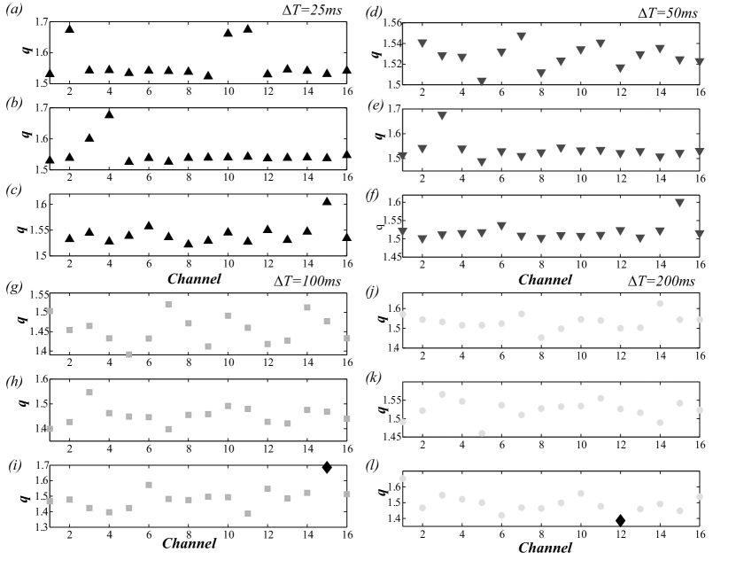
Figure 5: Parameter $q$ estimated through the fit of the firing distribution $Q_{q}(r)$ for the three different data sets. (a-c) $\Delta T$=25 ms; (d-f) $\Delta T$ = 50 ms; (g-i) $\Delta T$ = 100 ms (maximum observed $q$: black diamond in panel i, channel 15); and in (j-l) the time windows is $\Delta T$ =200ms (minimum observed $q$: black diamond in panel l, channel 12). The goodness of the fit was evaluated by estimating the normalised mean squared error (NMSE), $p-value<0.05$, see Appendix.

We estimated the normalised firing distribution $Q_{q}(r)$, for experimental data, by measuring the spiking rate in all non-overlapping windows of length $\Delta T$ (here 25, 50, 100, and 200 ms). We then fitted the parameter $q$, representing the extent of higher-order correlations present in the neuronal pool, to find the best-fitting function $Q_{q}(r)$ (as in Eq. (32)). Values of $q$ equal to unity imply the absence of higher-order correlations in the system. Fig 5 shows the fitted ${q}$ extracted for 3 different sets of 16 simultaneously recorded channels of multiunit activity, of increasing depth in the cortex (in 50 $\mu$m steps). For each set, the recordings were taken using different time windows $\Delta T=25$ ms (panels a-c), $\Delta T=50$ ms (panels d-f), $\Delta T=100$ ms (panels g-i) and $\Delta T=200$ ms (j-l). Notice that the maximum and minimum values of $q$ corresponds to channel 15 in panel i and channel 12 in panel l, respectively, for time windows of $\Delta T=100$ ms and $\Delta T=200$ ms.

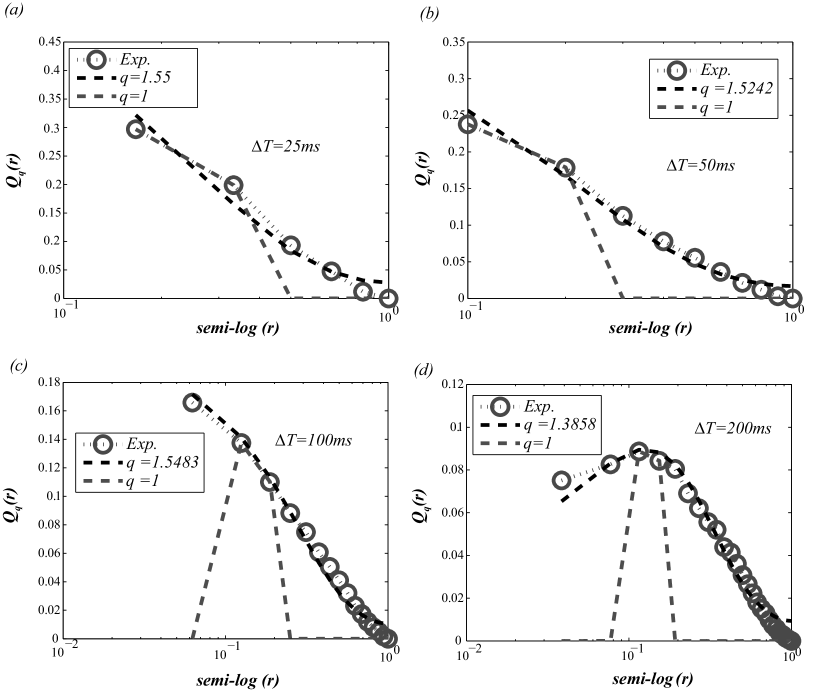
Figure 6: Fit of $Q_{q}(r)$ as a function of the normalised firing rate $r$ (semi-log in the X axis). (a) $\Delta T$=25 ms ($N_{max}=130$), $q=1.55$ and Fisher Info. equal to 0.1026 bits. b) $\Delta T$=50 ms ($N_{max}=160$), $q=1.5242$ and Fisher info. equal to 0.0489 bits. (c) $\Delta T$=100 ms ($N_{max}=200$), $q=1.5483$ and Fisher info. equal to 0.0151 bits. (d) $\Delta T$=200 ms ( $N_{max}=240$), $q=1.3858$ and Fisher info. equal to 0.0204 bits, which corresponds to the minimum observed $q$ (Fig 5 panel l: channel 12, diamond symbol). The goodness of the fit was evaluated by estimating the normalised mean squared error (NMSE), $p-value<0.05$. The theoretical approach considering $q>1$ (black dashed line) shows a remarkably good fit, in comparison to the case $q=1$ (grey dashed line), to the experimental curves (grey circles joined by dotted lines).

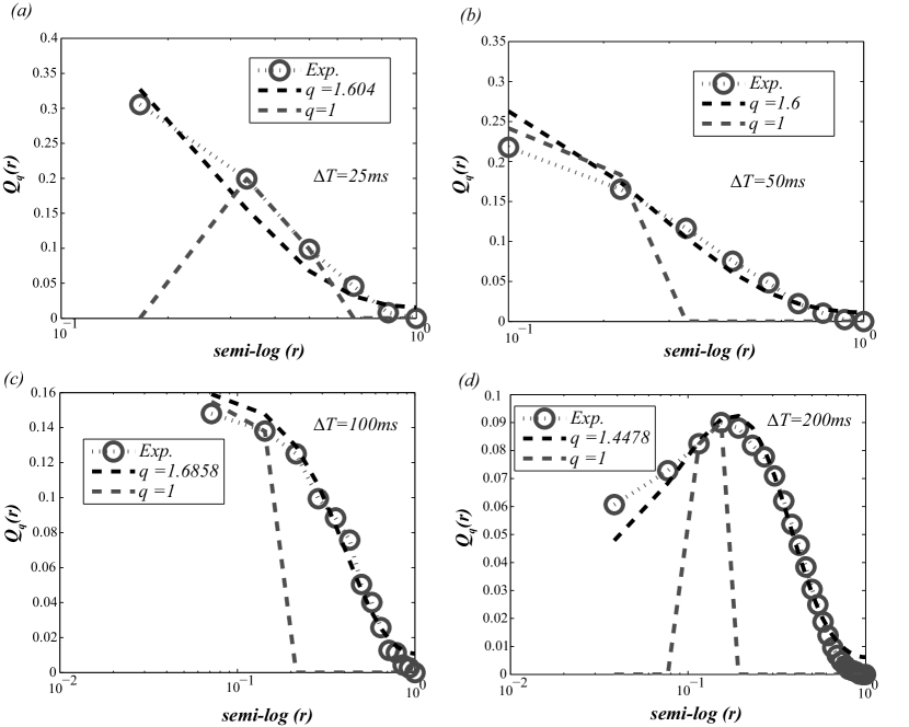
Figure 7: Fit of $Q_{q}(r)$ as a function of the normalised firing rate $r$ (semi-log in the X axis). (a) $\Delta T$=25 ms ($N_{max}=130$), $q=1.604$ and Fisher info. equal to 0.0905 bits. (b) $\Delta T$=50 ms ($N_{max}=140$), $q=1.6$ and Fisher info. equal to 0.0395 bits. (c) $\Delta T$=100 ms ($N_{max}=180$), $q=1.6858$ and Fisher info. equal to 0.0142 bits, which corresponds to the maximum observed $q$ (Fig 5 panel i: channel 15, diamond symbol). (d) $\Delta T$=200 ms ($N_{max}=240$ ), $q=1.4478$ and Fisher info. equal to 0.0150 bits. Same curve labels as in Fig 6.

In order to understand how well the model proposed in Eq. (32) fits the experimental data, we compared it with a fit with $q$ constrained to equal 1. We define the normalised firing rate as $r\equiv\frac{\langle k\rangle}{N_{max}}$, where $\langle k\rangle$ is the mean firing rate and $N_{max}$ is the maximum number of spikes. Figs 6 and  7 show the experimental spontaneous distribution of firing $Q_{q}(r)$ as a function of $r$ (on logarithmic scale) for those channels with the maximum and the minimum values of $q$, respectively. That is, we use the estimated $q$ and the parameters $\alpha$ and $h$ that give the best fit for the distribution. The optimisation fitting criterion is the normalised mean squared error (NMSE), and the default error value is lower than 0.05 ($p-value<0.05$). It is apparent that for all 25, 50, 100 and 200 ms time windows (Figs 6-7 a,b,c and d, respectively), the theoretical curve is a remarkably good fit to the experimental distribution ($p-value<0.05$ ). In contrast, the $q=1$ curve does not come close to modelling the data satisfactorily over a wide range of firing rates.

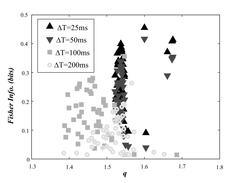
Figure 8: Fisher information versus $q$ (theoretical approach considering $q>1$), taking four different time windows and considering all the 48 available channels. Black up-triangles, $\Delta T$=25 ms; dark down-triangles, $\Delta T$=50 ms; dark grey squares, $\Delta T$=100 ms; light grey circles, $\Delta T$= 200 ms.

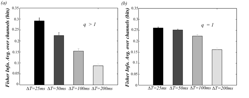
Figure 9: (a) Fisher information averaged over the 48 different channels (theoretical approach considering $q>1$). Black bar, $\Delta T$=25 ms; dark grey bar, $\Delta T$= 50 ms; grey bar, $\Delta T$=100ms; light grey bar, $\Delta T$=200ms. (b) Same as in B but considering the fit with $q$ constrained to be equal to 1.

To detect the dynamical changes in the probability distributions, we estimate Fisher information as in Eq.(34). On the one hand Fig 8 shows Fisher Information versus $q$ for the entire data set. Fig 9a shows Fisher information averaged over the 48 different channels, which becomes higher for smaller time windows. Notice from Fig 9b that when considering the case $q=1$, Fisher information takes higher values for 50, 100 and 200 ms time windows than for those in which $q>1$ is considered (Fig 9a). This is not the case for 25 ms time windows in which Fisher information takes a much higher value for $q>1$ than for those with $q$ constrained to be equal to 1. As expected, Fisher information is more substantial at shorter time windows, where the fine temporal precision at which the spikes may synchronise has a significant effect.

Overall our findings show that spontaneous distributions of firing with $q>1$ should be considered to accurately reproduce the experimental data set. The main advantage of this method is that through the inclusion of a deformation parameter $q$, which accounts for correlations higher than two within the probability distributions, we can quantify the degree of correlation and reproduce the experimental behaviour of the distribution of firing.

If we considered single neuron trial to trial fluctuations for a fixed stimulus in spike count fluctuations, the extent of noise correlations would depend on the width of the tuning curves as correlations come up from common inputs [42]. Thus, in this case Fisher information would depend on the sharpening of the distribution and also on the noise correlation, and therefore a sharper distribution would not necessarily imply a higher amount of Fisher information. This effect is shown, for instance, in Fig 7d ($\Delta T=200$ ms) and Fig 7b ($\Delta T=50$ ms); notice that d corresponds to a value of $q$ smaller than b. The firing distribution of Fig 7d has a higher slope than the one presented in Fig 7b, but this higher slope does not have a correspondence with a higher value of Fisher information (Fisher info equal to 0.0150 bits in Fig 7d, and Fisher Info equal to 0.0395 bits in Fig 7b).

Summing up, we presented a formalism that provides us with an estimate of the degree of correlation for the distribution of firing within pools of multiunit neural activity. This method allows us to naturally distinguish how far this distribution of firing is from the one we would obtain if each neuron contributes within CLT ($q=1$). It permits us, therefore, to quantify the amount of correlation significantly reducing the number of parameters associated with the correlation coordinates.

3.2 A Network simulation model

To test further our theoretical approach, we apply our formalism to a network simulation model in which the number for interconnected neurons is a parameter under control. We then analyse a simple network model in which neurons receive common overlapping inputs as in Fig 3, considering that each neuron can be interconnected randomly with more than two neurons. This will allow us to also test the hypothesis of Amari and collaborators that weak higher-order interactions of almost all orders are required to realise a widespread activity distribution of a large population of neurons [12].

The network simulation we use is the one developed in [46], which consists of cortical spiking neurons with axonal conduction delays and spike timing-dependent plasticity (STDP). Each neuron in the network is described by the simple spiking model [47]

$$v^{\prime}=0.04v^{2}+5v+140.u+I$$ (35)

$$u^{\prime}=a(bv-u)$$ (36)

with the auxiliary after-spike resetting

$$ifv\geq+30mV,then\begin{cases}v\leftarrow c\\ u\leftarrow u+d.\\ \end{cases}$$ (37)

Where $v$ is the membrane potential of the neuron, and $u$ is a membrane recovery variable, which accounts for the activation of $K+$ ionic currents and inactivation of $Na+$ ionic currents, and gives negative feedback to $v$. After the spike reaches its apex at +30 mV (not to be confused with the firing threshold) the membrane voltage and the recovery variable are reset according to Eq. (37). The variable $I$ accounts for the inputs to the neurons [47, 46].

Since we cannot simulate an infinite-dimensional system on a finite-dimensional lattice, we choose a network with a finite-dimensional approximation taking a time resolution of 1 ms. The network consists of $N=1000$ neurons with the first $Ne=650$ of excitatory RS type, and the remaining $Ni=350$ of inhibitory FS type [47]. Each excitatory neuron is connected to $M=2$,$3$,$20$,$40$,$60$,$80$,$100$,$120$,$140$ and $160$ random neurons, so that the probability of connection is $M/N=0.002$, $0.003$,$0.02$,$0.04$,$0.06$,$0.08$,$0.1$,$0.12$,$0.14$ and $0.16$. Each inhibitory neuron is connected to $M=2$,$3$,$20$,$40$,$60$,$80$,$100$,$120$,$140$ and $160$ excitatory neurons only. Synaptic connections among neurons have fixed conduction delays, which are random integers between 1 ms and 20 ms.

The main idea of this simulation is to investigate Amari’s hypothesis that correlations of almost all orders are needed to realise the widespread distribution of firing when a large number of neurons is considered and to show the behaviour of the parameter $q$ when the number of interconnected neurons is changed.

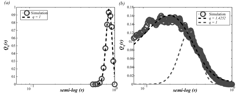
Figure 10: Distribution of firing $Q_{q}(r)$ versus the normalised firing rate $r$ (semi-log in the X axis), using 10 min of a simulated network that consists of $N=1000$ neurons with the first $Ne=650$ of excitatory RS type, and the remaining $Ni=350$ of inhibitory FS ($\Delta T$=25 ms). (a) Considering that each excitatory/inhibitory neuron is connected to $M=2$ or $3$ random neurons. We find no difference in the probability distribution of firing when $M=2$ or $M=3$ is considered, $q=1$. (b) Considering that the number of randomly interconnected neurons is $M=80$, $q=1.4252$. The goodness of the fit was evaluated by estimating the normalised mean squared error (NMSE), $p-value<0.05$.

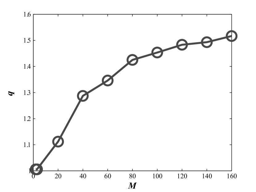
Figure 11: Parameter $q$ estimated through the fit of the firing distribution $Q_{q}(r)$, versus the number of interconnected neurons $M$. The goodness of the fit was evaluated estimating the normalised mean squared error (NMSE), $p-value<0.05$.

In order to show that the probability distribution in the thermodynamic limit is not realised even when pairwise interactions, or third-order interactions, exist, we estimate the joint probability distribution of firing when each excitatory/inhibitory neuron is interconnected to M=2 and 3 neurons. We run 10 minutes of simulated spiking activity, considering a window length of $\Delta T=25$ ms, which is a time window close to the one used by [43, 44, 2, 1] to investigate the effect of correlations. As shown in Fig 10a $q=1$ is a remarkably good fit to the simulated distribution of firing ($p-value<0.05$ ) when each excitatory/inhibitory neuron is connected to $M=2,3$ random neurons. Notice that we find no difference in the probability distribution of firing when M=2 and M=3 are considered. However, when the number of interconnected neurons becomes higher, the distribution of firing becomes more widespread (see Fig 10b) and $q$ increases as the number of interconnected neurons increases (Fig 11). In the current simulation we took 1000 neurons, however, when we chose 100-200 neurons, we were also able to capture the effect of the higher-order correlation if the parameter M was large enough to produce a widespread distribution (see Appendix, Section C).

4 Discussion and conclusions

Approaches using binary maximum entropy models at a pairwise level have been developed considering a very large number of neurons on short time scales [1, 2, 29]. These models can capture essential structures of the neural population activity, however, due to their pairwise nature their generality has been subject to debate [48, 49, 10]. In particular, using an information geometrical approach, E. Ohiorhenuan and J. D. Victor have shown the importance of the triplets to characterise scale dependence in cortical networks. They introduced a measure called “strain” that quantifies how a pairwise-only model must be “forced” to accommodate the observed triplet firing patterns [10]. Thus, although models accounting for pairwise interactions have proved able to capture some of the most important features of population activity at the level of the retina [1, 2], pairwise models are not enough to provide reliable descriptions of neural systems in general [48, 49, 10, 50, 51].

Very little is known about how the information saturates as the number of neurons increases. It has been pointed out by Amari and colleagues [12] that as the number of neurons increases, pairwise or triplet-wise correlations are not enough to realise a widespread distribution of firing. Understanding how neural information saturates as the number of neurons increases would require the development of an appropriate mathematical framework to account for correlations higher than two in the thermodynamic limit.

It is important, therefore, to develop an appropriate mathematical approach to investigate systems with a large number of neurons, which could account for correlations of almost all orders within the distribution of firing.

In this paper we present a theoretical approach to quantify the extent of higher than pairwise spike correlation in pools of multiunit activity when taking the limit of a very large number of neurons. In order to do this, we take advantage of recent mathematical progress on $q$-geometry to investigate, in the asymptotic limit, the effect of higher-order correlations on the probability distributions within the ECLT framework [21, 22, 23, 24, 25, 26]. The main basis of our formalism is that when taking the limit of a very large number of neurons within the framework of the CLT as in [12], we are losing information about higher-order correlations. Thus, in the new theoretical approach we take the limit of a very large number of neurons within the framework of the ECLT, instead of the CLT. The inclusion of a deformation parameter $q$ in the ECLT framework allows us to reproduce remarkably well the experimental distribution of firing and to avoid the sampling size problem of Eq. (2.1) due to the exponentially increasing number of parameters.

We estimated the normalised firing distribution $Q_{q}(r)$, from multiunit recordings, and fitted the parameter $q$ to find the best-fitting function $Q_{q}(r)$ (as in Eq. (32)). We showed by simple comparison how statistically different from the $q=1$ case the measured distribution is (as it is reduced to the CLT pairwise estimations of [12]). Our theoretical predictions provided a remarkably good fit for the experimental distribution. We showed that the parameter $q>1$ can capture higher-order correlations, which are salient features of the distribution of firing, when applied to our multiunit recording data obtained from mouse barrel cortex. As higher-order correlations were present in the data, the distributions in the CLT framework do not fit the experimental data well.

Staude and collaborators [52, 53, 54, 55] have introduced a quite powerful approach based on continuous-time point process to investigate higher-order correlations in non-Poissonian spike trains. Higher-order interactions are very important to investigate the neuronal interdependence in the cortex and at population level of the neuronal avalanches [27]. More specifically, Plenz and collaborators [27] have developed a very powerful theoretical framework based on a Gaussian interaction model that takes into account the pairwise correlations and event rates and by applying a intrinsic thresholding permit distinguishing higher order interactions. In this approach the pattern probabilities for the so-called “DG model” were estimated using the cumulative distribution of multivariate Gaussians and showed a high fitting precision of the experimental data. Our current theoretical formalism relies on a different basis: the recent progress made on the ECTL, and the main goal of our approach, is to provide a quantification of the amount of correlations higher than two when considering a large population of neurons. Thus using mathematical tools of non extensive statical mechanics [38, 24, 25, 26, 20, 32, 12, 33, 22, 23], we introduced an approach that provides a quantification of the degree of higher order correlation for a very large number of neurons.

It would be interesting to develop in the close future a paper showing a careful comparison of our current method with the one developed by Plenz and collaborators. This would help to investigate the possible link of the quantification through the $q$ parameter with the “DG model”[27] and to gain more insights for future analysis. Evaluating the degree of $q$ can help to understand further the processing of information in the cortical network and to get more understanding of the non-linearities of information transmission within a neuronal ensemble. Although formally speaking the multiunit recordings are not in the“thermodynamic limit”, the current methodology presented in this paper is a completely new theoretical approach for theoretical neuroscience. And as more data become available for a very large number of neurons, i.e. including evoked activity to sensory stimuli, our theoretical approach could provide an important mathematical tool to evaluate important questions such as how quickly neural information saturates as the number of neurons increases, and whether it saturates at a level much lower than the amount of information available in the input.

The pooling process can be taken to reflect the behaviour of a simple integrate-and-fire neuron model in reading out the activity of an ensemble of neurons, or alternately the recording of multiunit neural activity, without spike sorting. As we cannot know what the exact number of neurons in our multiunit recordings is, we approximated this number by the maximum number of spikes. In the pooling approach we developed within the ECLT framework we assumed the asymptotic limit of a very large number of neurons. Our method was developed within the information geometry framework, similar to that described in [10]. However, it is important to remark three important differences between the method developed in [10] and our current theoretical approach: first, we assumed homogeneity across neurons; second, our approach was developed assuming a very large number of neurons within the ECLT framework, and third, our approach accounted for cases in which a widespread probability distribution is not realised even when pairwise interactions, or third-order interactions, exist. The significance of our approach is that it allows us to extend analytically solvable models of the effect of correlations higher than two and to compute their scaling properties in the case of a very large number of neurons. Our treatment provides a quantification of the degree of correlation within the probability distribution, which is summarised in a single $q$ parameter, thus avoiding the sample size problem that constitutes the main intractability reason of the approaches presented in Eq. (2.1).

To contrast our current data analysis with a case in which the network structure is known a priori, we tested our theoretical approach using a network simulation model in which the number for interconnected neurons is a parameter under control. We then analysed a simple network model in which neurons receive common overlapping inputs and considering that each neuron can be interconnected randomly with more than two neurons. We showed that in the specific network model, high connectivity is required to get a widespread distribution, which is in agreement with the hypothesis of Amari [12] that weak higher-order interactions of almost all orders are required for realising a widespread activity distribution in the “thermodynamic limit” [12]. Moreover, our results are in agreement with the hypothesis of Amari and colleagues [12] that the widespread probability distribution in the thermodynamic limit is not realised even when pairwise interactions, or third-order interactions, exist. Correlations of almost all orders are then needed to realise the widespread activity distribution of a very large population of neurons. In our current simulation we took 1000 neurons, which may be considered quite a large number in comparison to the number of neurons that a multiunit recording might capture. However, when we chose 100-200 neurons in our simulation, we were also able to capture the effect of the higher-order correlation if the number of interconnected neurons was large enough to produce a widespread distribution (see Appendix, section C). Thus, as higher-order correlations were present in the simulated data set, a very weird network architecture will be required to force $q=1$, and thus in this case the distribution of firing in the CTL framework does not come even close to fitting the simulated data.

The model we developed using an information - geometric approach within the ECLT framework, and together with Fisher information estimations, in principle could allow population codes involving higher-order correlations to be studied in the thermodynamic limit, in the same way as other authors have done for the second order case [56, 42, 57]. This is particularly interesting as in most cases pairwise models do not provide reliable descriptions of true biological systems [49]. Thus our approach could be of help to gain further insights into the role of high-order correlations in information transmission for very large systems, and could also be an important mathematical tool to evaluate whether the evoked activity may induce plasticity effects on the network when compared to the spontaneous signal. Applying our formalism to a data set obtained from mouse barrel cortex using multiunit recordings, we showed that a simple estimation of the deformation parameter $q$ attached to the probability distribution of firing can answer us how significant the degree of higher-order spike correlations is within pools of neural activity. In our current analysis we show that higher - order correlations are prevalent but they do not, in general, improve the accuracy of the population code when considering a large number of neurons. Overall our findings show that Fisher information increases as the time window decreases, which would involve an easier discrimination task when the time windows become shorter.

Summarising, we presented an information-geometric approach to quantify the degree of spike correlations higher than two in pools of multiunit neural activity. Our proposed formalism provides a statistical characterisation of the amount of high-order correlations through the $q$ parameter, avoiding the sampling problem of the pooling approach when high-order correlations in the thermodynamic limit are considered.

5 Materials and methods

Recordings were made from adult female C56BL/6 mice, of 2-3 months of age. The animals were maintained in the Imperial College animal facility and used in accordance with UK Home Office guidelines. The experiments were approved by the UK Home Office, under Project License 70/6516 to S. R. Schultz. Mice were sedated by an initial intraperitoneal injection of urethane (1.1 g/kg, 10 % w/v in saline) followed by an intraperitoneal injection of 1.5 ml/kg of Hypnorm/Hypnovel (a mix of Hypnorm in distilled water 1:1 and Hypnovel in distilled water 1:1; the resulting concentration being Hypnorm:Hypnovel:distilled water at 1:1:2 by volume), 20 minutes later. Atropine (1 ml/kg, 10 % in distilled water) was injected subcutaneously. Further supplements of Hypnorm (1 ml/kg, 10 % in distilled water) were administered intraperitoneally if required. Their body temperature was maintained at $37\pm 0.5^{\circ}$C with a heating pad. A tracheotomy was performed and an endotracheal tube (Hallowell EMC) was inserted to maintain a clear airway as previously described [58]. After the animal was fixed on stereotaxic frame, a craniotomy was performed, aimed at above barrel C2. A small window on the dura was exposed to allow insertion of the multi-electrode array. The exposed cortical surface was covered with artificial cerebrospinal fluid (in mM: 150 NaCl, 2.5 KCl, 10 HEPES, 2 CaCl2, 1 MgCl2; pH 7.3 adjusted with NaOH) to prevent drying. The linear probe (model: A1x16-3mm-50-413, NeuroNexus Technologies) was lowered into the brain perpendicularly to the cortical surface, until all 16 electrode sites were indicating multiunit neural activity, and allowed to settle for 30 minutes before recording began.

Appendix

A. Estimation of ${F_{q}(\varepsilon)}$ and $Q_{q}(r)$

We take the limit of $N\rightarrow\infty$, in the “ECLT framework” [22, 23, 24, 25, 26], instead of the Gaussian CLT as considered in [12], we can define:

$${F_{q}(\varepsilon)}\equiv P_{r}(u>0|\varepsilon) = P_{r}(u_{i}>\frac{h-\sqrt{\alpha}\varepsilon}{\sqrt{1-\alpha}})$$

$$= \frac{1}{\sqrt{2\pi}}\int_{\frac{h-\sqrt{\alpha}\varepsilon}{\sqrt{1-\alpha}}}^{\infty}\!\exp_{q}{(-\frac{v^{2}}{2})}\,dv$$

Notice that if we consider the limit of the CLT ($q=1$), the previous expression reduces to

$${F_{q=1}(\varepsilon)}=\frac{1}{2}\mathrm{Erfc}(\frac{1}{\sqrt{2}}\frac{h-\sqrt{\alpha}\varepsilon}{\sqrt{1-\alpha}}).$$ (A-2)

where $\mathrm{Erfc(x)}=\frac{2}{\sqrt{\pi}}\int_{x}^{\infty}\exp(-t^{2})dt$ denotes the complementary error function. However, if the effect of higher order correlations than two are not negligible then according to the ECTL $q>1$, thus

$$\exp_{q}(-\frac{v^{2}}{2})=\frac{1}{\Gamma(\frac{1}{q-1})}\int_{0}^{\infty}dt\,t^{\frac{1}{q-1}-1}\exp({-t-t(q-1)\frac{v^{2}}{2}})$$ (A-3)

which is known as Hilhorst transform [37], an integral representation widely used in generalized statistical mechanics [38]. Thus $F_{q}(\varepsilon)$ reads

$$\begin{split}{F_{q}(\varepsilon)}=\frac{1}{\Gamma(\frac{1}{q-1})}\int_{0}^{\infty}\int_{\frac{h-\sqrt{\alpha}\varepsilon}{\sqrt{1-\alpha}}}^{\infty}dt\,dv\,t^{\frac{1}{q-1}-1}\exp({-t+t(q-1)\frac{v^{2}}{2}})\end{split}$$ (A-4)

and substituting $w={{\sqrt{\frac{t(q-1)}{2}}}}v$, we can rewrite

$$\begin{split}\int_{\frac{h-\sqrt{\alpha}\varepsilon}{\sqrt{1-\alpha}}}^{\infty}dv\exp\left({-t-t(q-1)\frac{v^{2}}{2}}\right)=\frac{\exp\left({-t}\right)}{\sqrt{\frac{t(q-1)}{2}}}\frac{\sqrt{\pi}}{2}\left(1-\mathrm{Erf}\left[\sqrt{\frac{t(q-1)}{2}}\left(\frac{h-\sqrt{\alpha}\varepsilon}{\sqrt{1-\alpha}}\right)\right]\right)\end{split}$$ (A-5)

where $\mathrm{Erf(x)}$ denotes the error function,

$$\mathrm{Erf}(x) = 1-\frac{\Gamma(\frac{1}{2},x^{2})}{\sqrt{\pi}}$$ (A-6)

$$= \frac{2}{\sqrt{\pi}}\int_{0}^{x}\exp(-t^{2})dt$$

and

$$\Gamma(\frac{1}{2},x^{2})=2\int_{x}^{\infty}\exp({-t^{2}})dt.$$ (A-7)

Thus, using

$$\begin{split}\int_{0}^{\infty}x^{\mu-1}\exp({-\beta x})\,\Gamma(\nu,\alpha x)dx={\frac{\alpha^{\nu}\Gamma(\mu+\nu)}{\mu(\alpha+\beta)^{\mu+\nu}}}\,{{}_{2}F_{1}}(1,\mu+\nu,\mu+1;\frac{\beta}{\alpha+\beta})\end{split}$$

in Eq. (A. Estimation of ${F_{q}(\varepsilon)}$ and $Q_{q}(r)$) where $Re(\alpha+\beta)>0$,$Re(\mu)>0$, $Re(\mu+\nu)>0$ and ${}_{2}F_{1}$ denotes the Gauss hypergeometric function, we can derive a compact expression for $F_{q}$ as

$$\begin{split}{F_{q}(\varepsilon)}=\zeta(\varepsilon)\,{{}_{2}F_{1}(1,\frac{1}{q-1};\frac{1}{q-1}+\frac{1}{2};\frac{1}{1+\xi_{0}(\varepsilon)})}\end{split}$$ (A-8)

where we named

$$\zeta(\varepsilon)=\frac{\sqrt{\xi_{0}(\varepsilon)}}{{2\sqrt{2\pi}}(\frac{1}{q-1}-\frac{1}{2})\sqrt{\frac{q-1}{2}}(1+\xi_{0}(\varepsilon))^{\frac{1}{q-1}}}$$ (A-9)

and

$$\xi_{0}(\varepsilon)=\frac{(q-1)(h-\sqrt{\alpha}\varepsilon)^{2}}{2({1-\alpha})}.$$ (A-10)

Making use of the fact that the hypergeometric functions accomplish the following identity

$${{}_{2}F_{1}(a,b;c;z)}={{}_{2}F_{1}(b,a;c;z)}=(1-z)^{c-a-b}{{}_{2}F_{1}(c-a,c-b;c;z)}$$ (A-11)

(see [59]), we can name: $a=1$; $b=\frac{1}{q-1}$;$c=\frac{1}{q-1}+\frac{1}{2}$;$z=\frac{1}{1+\xi_{0}(\varepsilon)}$ and therefore

$${{}_{2}F_{1}(1,\frac{1}{q-1};\frac{1}{q-1}+\frac{1}{2};\frac{1}{1+\xi_{0}(\varepsilon)})}=(\frac{\xi_{0}(\varepsilon)}{1+\xi_{0}(\varepsilon)})^{-\frac{1}{2}}{{}_{2}F_{1}(\frac{1}{q-1}-\frac{1}{2},\frac{1}{2};\frac{1}{q-1}+\frac{1}{2};\frac{1}{1+\xi_{0}(\varepsilon)})}.$$ (A-12)

Then Eq. (A-8) reads as,

$$\begin{split}{F_{q}(\varepsilon)}=\frac{1}{{2\sqrt{2\pi}}(\frac{1}{q-1}-\frac{1}{2})\sqrt{\frac{q-1}{2}}(1+\xi_{0}(\varepsilon))^{\frac{1}{q-1}-\frac{1}{2}}}\,{{}_{2}F_{1}(\frac{1}{q-1}-\frac{1}{2},\frac{1}{2};\frac{1}{q-1}+\frac{1}{2};\frac{1}{1+\xi_{0}(\varepsilon)})}.\end{split}$$ (A-13)

Notice that the incomplete beta function [59] is defined as

$$\begin{split}{B_{w}(p,q)}=\int_{0}^{w}t^{p-1}(1-t)^{q-1}dt=\frac{1}{p}w^{p}\,{{}_{2}F_{1}(p,1-q;p+1,w)}\end{split}$$ (A-14)

and therefore naming $p=\frac{1}{q-1}-\frac{1}{2}$,$q=\frac{1}{2}$ and $w=\frac{1}{1+\xi_{0}(\varepsilon)}$ we can rewrite

$$\begin{split}{B_{\frac{1}{1+\xi_{0}(\varepsilon)}}(\frac{1}{q-1},\frac{1}{2})}=\frac{1}{(\frac{1}{q-1}-\frac{1}{2})(1+\xi_{0}(\varepsilon))^{\frac{1}{q-1}-\frac{1}{2}}}\,{{}_{2}F_{1}(\frac{1}{q-1}-\frac{1}{2},\frac{1}{2};\frac{1}{q-1}+\frac{1}{2};\frac{1}{1+\xi_{0}(\varepsilon)})}.\end{split}$$ (A-15)

This allows us to rewrite ${F_{q}(\varepsilon)}$ in terms of a beta incomplete function with dependence on $q$, as

$$\begin{split}{F_{q}(\varepsilon)}=\frac{1}{{2\sqrt{2\pi}}\sqrt{\frac{q-1}{2}}}{B_{\frac{1}{1+\xi_{0}(\varepsilon)}}(\frac{1}{q-1},\frac{1}{2})}.\end{split}$$ (A-16)

The distribution of firing is approached as

$$Q_{q}(r) \simeq NP_{r}\{r=\frac{k}{N}\}$$ (A-17)

$$= NE_{\varepsilon}\{\left(\begin{array}[]{c}N\\ k\end{array}\right)[{F_{q}(\varepsilon)}]^{k}[1-F_{q}(\varepsilon)]^{N-k}\}.$$ (A-20)

Using that, $\left(\begin{array}[]{c}N\\ k\end{array}\right)\cong\frac{\exp{(-Nr\log(r)-N(1-r)\log(1-r))}}{\sqrt{2\pi Nr(1-r)}}$ in the limit of large $N$ we can write

$$\begin{split}Q_{q}(r)=\sqrt{\frac{N}{(2\pi)^{2}r(1-r)}}\int_{-\infty}^{\infty}d\varepsilon\\ \exp\{{N[r\log(\frac{{F_{q}(\varepsilon)}}{r})+(1-r)\log(\frac{1-{F_{q}(\varepsilon)}}{1-r})]-\frac{{\varepsilon}^{2}}{2}}\}\end{split}$$ (A-21)

But notice that, in the definition of $Q_{q}(r)$ the standard exponential is used since the correlation effects were previously included through the deformation parameter $q$ within ${F_{q}(\varepsilon)}$ (where we have used the ECLT [24]). The previous integral (Eq. A-21) is solved using the saddle point approximation [39, 12], and then Eq. (32) is obtained. The goodness of the fit was evaluated estimating the normalised mean squared error (NMSE), $p-value<0.05$. It is then fitted the $q$ parameter to get the best fitting function $Q_{q}(r)$ in Eq. (32) for the experimental distribution. We used the matlab subroutine GFIT2 to compute goodness of fit, for regression model, given matrix/vector of target and output values.

B. The Gaussian Distribution within the q-Information Geometry framework

The q-Gaussian distribution is defined as:

$$p(x,\mu,\sigma)=\exp_{q}(-\frac{(x-\mu)^{2}}{2\sigma^{2}}-\psi(\mu,\sigma)),$$ (B-1)

which can be rewritten as:

$$p(x,\mu,\sigma)=\exp_{q}(\frac{\mu}{\sigma^{2}}x-\frac{(x)^{2}}{2\sigma^{2}}-\frac{(\mu)^{2}}{2\sigma^{2}}-log_{q}(\sqrt{2\pi})).$$ (B-2)

where can identify the correlation coordinates as

$$\theta_{1}=\frac{\mu}{\sigma^{2}},$$ (B-3)

$$\theta_{2}=\frac{-1}{2\sigma^{2}},$$ (B-4)

and the factor

$$\psi=\frac{(\mu)^{2}}{2\sigma^{2}}+log_{q}(\sqrt{2\pi}\sigma).$$ (B-5)

C. Simulation

We applied our formalism to a network simulation model in which the number of neurons is a parameter under control. In the following que consider a network of N = 200 neurons with the first Ne = 80 of excitatory RS type, and the remaining Ni=120 of inhibitory FS type [47]. Each excitatory neuron is connected to M=80 random neurons, and each inhibitory neuron is connected to M=80 excitatory neurons only. Synaptic connections among neurons have fixed conduction delays of 10 ms. Notice that weak higher-order interactions of almost all orders are required for realising a widespread activity distribution of a large population of neurons [12], this is in agreement with the hypothesis of Amari a[12] that the widespread probability distribution in the thermodynamic limit is not realised even when pairwise interactions, or third-order interactions, exist (see Fig.  C.1 ).

Figure 1: Schematic representation of spike correlations. (a) Spikes being fired at a given time window of size $\Delta t$ considering a population of $N$ neurons.(b)$E(a_{1})$, $E(a_{2})$ and $E(a_{3})$ are the family of distributions having the same correlation coordinates $a_{1}$, $a_{2}$, and $a_{3}$, respectively. The family of all probability distributions belongs to the $q$-exponential family of distributions for any $q$, and thus we can introduce the $q$-geometrical structure to any arbitrary family of probability distributions.

Figure 2: $E(a_{1})$, $E(a_{2})$ and $E(a_{3})$ are the family of distributions having the same correlation coordinates $a_{1}$, $a_{2}$, and $a_{3}$, respectively. The family of all probability distributions belongs to the $q$-exponential family of distributions for any $q$, and thus we can introduce the $q$-geometrical structure to any arbitrary family of probability distributions.

Figure 3: Schematic representation of a neuronal pool with $N$ neurons that receives $s_{1},s_{2},...s_{m}$ common inputs.

Figure 4: Distribution of firing $Q_{q}(r)$ computed for $q=1$ and $q=1.3$ (semi-log in the X axis).

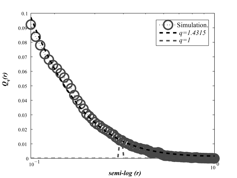
Figure C.1: Distribution of firing $Q_{q}(r)$ using 10 min of simulated network which consists of N = 200 neurons with the first Ne = 80 of excitatory RS type, and the remaining Ni=120 of inhibitory FS ($\Delta T$=25 ms). Considering that the number of randomly interconnected neurons is M=80, $q=1.4315$. The goodness of the fit was evaluated estimating the normalised mean squared error (NMSE), $p-value<0.05$.

References

- [1] E. Schneidman, M. J. Berry, R. Segev, and W. Bialek. Weak pairwise correlations imply strongly correlated network states in a neural population. Nature 440 (2006) 1007–1012.
- [2] J. Shlens, G.D. Field, J. L. Gauthier, M. I. Grivich, D. Petrusca, A. Sher, A. M. Litke, and E.J. Chichilnisky. The structure of multi-neuron firing patterns in the primate retina. J. Neurosci. 26 (2006) 8254–8266.
- [3] J. M. Alonso, C.-I. Yeh, and C. R. Stoelzel. Visual stimuli modulate precise synchronous firing within the thalamus. Thalamus Relat. Sys. 4 (2008) 21–34.
- [4] A. Kohn and M. Smith. Stimulus dependence of neuronal correlation in primary visual cortex of the macaque. J. Neurosci. 25 (2005) 3661–3673.
- [5] J. Samonds and A. Bonds. Gamma oscillation maintains stimulus structure dependent synchronization in cat visual cortex. J. Neurophysiol. 93 (2005) 223–236.
- [6] F. Montani, A. Kohn, M. Smith, and S. Schultz. The role of correlations in direction and contrast coding in the primary visual cortex. J Neurosci. 27 (2007) 2338–48.
- [7] S. R. Schultz, K. Kitamura, J. Krupic, A. Post-Uiterweer, and M. Häusser. Spatial pattern coding of sensory information by climbing-fiber evoked calcium signals in networks of neighboring cerebellar purkinje cells. J. Neurosci. 29 (2009) 8005–8015.
- [8] A. K. Wise, N. L. Cerminara, D. E. Marple-Horvat, and R. Apps. Mechanisms of synchronous activity in cerebellar Purkinje cells. J. Physiol. 588 (2010) 2373–2390.
- [9] F. Montani, R. Ince, R. Senatore, E. Arabzadeh, M. Diamond, and S. Panzeri. The impact of high-order interactions on the rate of synchronous discharge and information transmission in somatosensory cortex. Phil. Trans. R. Soc. A 367 (2009) 3297–3310.
- [10] I. Ohiorhenuan and J. Victor, Information-geometric measure of 3-neuron firing patterns characterizes scale-dependence in cortical networks, J Comput Neurosci. 30 (2010) 125–141.
- [11] D. Hebb. The organisation of behaviour. New York: Wiley and Sons, 1949.
- [12] S. Amari, H. Nakahara, S. Wu, and Y. Sakai. Synchronous firing and higher order interactions in neuron pool. Neural Computation 15 (2003) 127–142.
- [13] S. Bohte, H. Spekreijse, and P. Roelfsema. The effects of pair-wise and higherorder correlations on the firing rate of a postsynaptic neuron. Neural Computation 12 (2000) 153–159.
- [14] S. Amari. Information geometry on hierarchy of probability distributions. IEEE Transactions on Information Theory 47 (2001) 1701–1711.
- [15] S. Nakahara and S. Amari. Information geometric measure for neural spikes. Neural Computation 14 (2002) 2269–2316.
- [16] T. Tanaka. Information geometry of mean-field approximation. Neural Computation 12 (2000) 1951–1968.
- [17] S. Ikeda, T. Tanaka, and S. Amari. Stochastic reasoning, free energy, and information geometry. Neural Computation 16 (2004) 1179–1810.
- [18] S. Wu, S. Amari, and H. Nakahara. Information processing in a neuron ensemble with the multiplicative correlation structure. Neural Networks 17 (2004) 205–214.
- [19] S. Amari. Theory of information space: a differential-geometric foundation of statistic. Post RAAG Reports 106 (1980).
- [20] S. Amari and H. Nagaoka. Methods of Information Geometry Translations of Mathematical Monographs 191, Oxford University Press, 2000.
- [21] S. Amari and A. Ohara. Geometry of q-exponential family of probability distributions. Entropy 13 (2011) 1170–1185.
- [22] S. Umarov, C. Tsallis, and S. Steinberg. On a q-central limit theorem consistent with nonextensive statistical mechanics. Milan Journal of Mathematics 76 (2008) 307–328.
- [23] S. Umarov, C. Tsallis, M. Gell-Mann, and S. Steinberg. Generalization of Symmetric -Stable Lévy distributions for . J. of Math. Phys. 51 (2010) 033502.
- [24] C. Vignat and A. Plastino. Central limit theorem and deformed exponentials. J. Phys. A: Math. Theor. 40 (2007) F969–F978.
- [25] C. Vignat and A. Plastino. Estimation in a fluctuating medium and power-law distributions. Phys. Lett. A 360 (2007) 415–418.
- [26] C. Vignat and A. Plastino. Scale invariance and related properties of q-Gaussian systems. Physics Letters A 365 (2007) 370–375.
- [27] S. Yu, H. Yang, H. Nakahara, G.S. Santos, D. Nikolic, and D. Plenz. Higher-order interactions characterized in cortical activity. Journal Neuroscie. 31 (2011) 17514–17526.
- [28] G. Tkacik, E. Schneidman, M.J. Berry II and W. Bialek. Ising models for networks of real neurons. qbio.NC/0611072, 2006.
- [29] J. Shlens, G. D. Field, J. L. Gauthier, M. Greschner, A. Sher, A. Litke, and E. Chichilnisky. The structure of large-scale synchronized firing in primate retina. J.Neurosci. 29 (2009) 5022–5031.
- [30] W. Feller. An Introduction to Probability Theory and Its Applications, vol. 3rd Edition. John Wiley and Sons, 2008.
- [31] S. M. Ross. A First Course in Probability, vol. 2nd Edition. Macmillan Publishing Company, 1976.
- [32] C. Tsallis, M. Gell-Mann, and Y. Sato. Asymptotically scale-invariant occupancy of phase space makes the entropy extensive. PNAS 102 (2005) 15377–15382.
- [33] M.P.H. Stumpf and M.A. Porter. Critical Truths About Power Laws. Science 335 (2012) 665–666.
- [34] Generalized Box-Müller Method for Generating -Gaussian Random Deviates. IEEE Transactions on Information Theory 53 (2007) 4805–4810.
- [35] F Büyükiliça, D Demirhana, and A. Güleç. A statistical mechanical approach to generalized statistics of quantum and classical gases. Phys. Lett. A 197 (1994) 209–220.
- [36] S. Martinez, F. Pennini, A. Plastino, and M. Portesi. q-thermostatistics and the analytical treatment of the ideal fermi gas. Physica A 332 (2004) 230–248.
- [37] I. S. Gradsteyn and I. Ryzhik. Table of Integrals, Series and Products (Seventh Edition). Academic Press, 2007.
- [38] C. Tsallis. In New Trends in Magnetism, Magnetic Materials and Their Applications. eds. Morán-Lopez, J.L. and Sánchez J.M., (Plenum, New York, 1994), p. 451.
- [39] R. Butler. Saddlepoint approximations with applications. Cambridge Series in Statistical and Probabilistic Mathematics, Cambridge University Press, 2007.
- [40] Y. Linnik. An information-theoretic proof of the central limit theorem with the lindeberg condition. Theory Probab. Appl. 4 (1959) 288–299.
- [41] G. I. Ferri, F. Pennini, and A. Plastino. LMC - complexity and various chaotic regimes. Phys. Lett. A 373 (2009) 2210–2214.
- [42] P. Seriès, P.E. Latham, and A. Pouget. Tuning curve sharpening for orientation selectivity: coding efficiency and the impact of correlations. Nature Neuroscience 7 (2004) 1129–1135.
- [43] S. Panzeri, S. Schultz, A. Treves, and E.T Rolls. Correlations and the encoding of information in the nervous system. Proc. R. Soc. Lond. B. Biol. Sci. 266 (1999) 1001–1012.
- [44] S. Panzeri, H. Golledge, F. Zheng, M. Tovée, and M.P. Young. Objective assessment of the functional role of spike train correlations using information measures. Visual Cognition 8 (2001) 531–547.
- [45] A. Treves, S. Panzeri, E. T. Rolls, and E. Wakeman. Firing rate distributions and eficiency of information transmission of inferior temporal cortex neurons to natural visual stimuli. Neural Computation 11 (1999) 601–631.
- [46] E. M. Izhikevich. Polychronization: Computation with spikes. Neural Computation 18 (2006) 245–282.
- [47] E. M. Izhikevich. Simple model of spiking neurons. IEEE Transactions on Neural Networks 14 (2003) 1569–1572.
- [48] P. Berens and M. Bethge. Near-maximum entropy models for binary neural representations of natural images. In Proceedings of the Twenty-First Annual Conference on Neural Information Processing Systems, Cambridge, MA, MIT Press. 20 (2008) 97–104.
- [49] Y. Roudi, S. Nirenberg, and P. Latham. Pairwise maximum entropy models for studying large biological systems: when they can work and when they can t. PLoS Comput. Biol. 5 (2009) e1000380.
- [50] I. Ohiorhenuan, K. Mechler, F.and Purpura, A. Schmid, Q. Hu, and J. Victor. Sparse coding and high-order correlations in fine-scale cortical networks. Nature 466 (2010) 617–622.
- [51] E. Ganmor, R. Segev, and E. Schneidman. Sparse low-order interaction network underlies a highly correlated and learnable neural population code. PNAS 108 (2011) 9679–9684.
- [52] W. Ehm, B. Staude, and S. Rotter. Decomposition of neuronal assembly activity via empirical de-poissonization. Electr. J. Stat. 1 (2007) 473–95.
- [53] B. Staude, S. Grün, and S. Rotter. Higher-order correlations in non-stationary parallel spike trains: statistical modeling and inference. Front. Comput. Neurosci. 29 (2010) 327–50.
- [54] B. Staude, S. Rotter, S. Grün. CuBIC cumulant based inference of higher order correlations in massively parallel spike trains. J. Comput Neurosci. 29 (2010) 327–350.
- [55] I. Reimer, B. Staude, W. Ehm, and S. Rotter. Modeling and analyzing higher order correlations in non-poissonian spike trains. Journal of Neuroscience Methods 208 (2012) 18–33.
- [56] L. Abbott and P. Dayan. The effect of correlated variability on the accuracy of a population code. Neural Computation 11 (1999) 91–101.
- [57] B. B. Averbeck, P. E. Latham, and A. Pouget. Neural correlations, population coding and computation. Nat. Rev. Neurosci. 7 (2006) 358–366.
- [58] O. Moldestad, P. Karlsen, S. Molden, and J. Storm. Tracheotomy improves experiment success rate in mice during urethane aneasthesia and stereotaxic surgery. J. Neurosci. Methods 176 (2009) 57–62.
- [59] A. Erdélyi, W. Magnus, F. Oberhettinger, and F.G. Tricomi. Higher transcendental functions. Vol. I., McGraw Hill, 1953.