Momentum dependence of the bispectrum in two-field inflation

Abstract

We examine the momentum dependence of the bispectrum of two-field inflationary models within the long-wavelength formalism. We determine the sources of scale dependence in the expression for the parameter of non-Gaussianity $f_{\mathrm{NL}}$ and study two types of variation of the momentum triangle: changing its size and changing its shape. We introduce two spectral indices that quantify the possible types of momentum dependence of the local type $f_{\mathrm{NL}}$ and illustrate our results with examples.

LPT-12-116

1 Introduction

The study of inflationary non-Gaussianities and their impact on the cosmic microwave background has been an important subject of cosmological research in recent years. In nine years of WMAP data [1] and one year of data from the Planck satellite [2] no primordial non-Gaussianity of the local and equilateral types (see below) was observed, and constraints have tightened considerably. Next year’s Planck release is expected to put even tighter constraints on those types of non-Gaussianity, as well as investigate many additional types (which differ in their momentum dependence). The importance of the current constraints and a future possible detection or further improvements of the constraints lies in the fact that they allow us to discriminate between different classes of models of inflation, since these predict different types and amounts of non-Gaussianity.

There are basically two distinct types of non-Gaussianity that are most important from the point of view of inflation: the equilateral type produced at horizon-crossing, which has a quantum origin and is maximal for equilateral triangle configurations [3], and the local type produced outside the inflationary horizon due to the existence of interacting fields. The latter is maximized for squeezed triangles, i.e.  isosceles triangles with one side much smaller than the other two [4, 5]. The first type is known to be slow-roll suppressed for single-field models with standard kinetic terms and trivial field metric [6]. On the other hand, some models with non-standard kinetic terms coming from higher-dimensional cosmological models are known to produce non-Gaussianity of the equilateral type so large that it is not compatible with WMAP and Planck observations [7, 8, 9, 10], thus leading people to consider an extra field in order to achieve smaller values of the parameter $f_{\mathrm{NL}}$ of non-Gaussianity.

Non-Gaussianity of the squeezed type can be found naturally in multiple-field models of inflation [11, 12], due to the sourcing of the adiabatic mode by the isocurvature components outside the horizon. For single-field models this is obviously impossible due to the absence of isocurvature modes. There has been much study of two-field models [13, 14, 15, 16, 17, 18, 19, 20], being the easiest to investigate, in the hope of finding a field potential that can produce local non-Gaussianity large enough to be measurable in the near-future. It proves to be non-trivial to sustain the large non-Gaussianity produced during the turn of the fields until the end of inflation.

Non-Gaussianity produced at horizon-crossing is known to be momentum-dependent. The scale dependence of the equilateral $f_{\mathrm{NL}}$ produced for example from DBI inflation [21, 22, 9, 23, 24], has been examined both theoretically [25, 26, 27, 28] and in terms of observational forecasts [29, 30]. In this paper we are going to study the scale dependence of local-type models that has not been studied as much. Squeezed-type non-Gaussianity, produced outside the horizon, is usually associated with a parameter of non-Gaussianity $f_{\mathrm{NL}}^{\mathrm{local}}$ that is local in real space, and therefore free of any explicit momentum dependence, defined through $\zeta(x)=\zeta_{L}(x)+(3/5)f_{\mathrm{NL}}^{\mathrm{local}}(\zeta_{L}(x)^{2}-\langle\zeta_{L}(x)\rangle^{2})$, where $\zeta_{L}$ is the linear Gaussian part. Nevertheless, calculations of $f_{\mathrm{NL}}$ for several types of multiple-field models (see e.g.  [19, 31, 20]) show that there is always a momentum dependence inherited from the horizon-crossing era, which can in principle result in a tilt of $f_{\mathrm{NL}}$. When a physical quantity exhibits such a tilt one usually introduces a spectral index, as for example in the case of the power spectrum. The observational prospects of the detection of this type of scale dependence of local $f_{\mathrm{NL}}$ were studied in [30]. Only recently spectral indices for $f_{\mathrm{NL}}$ were defined in [32, 33, 34], keeping constant the shape of the triangle or two of its sides, within the $\delta N$ formalism. Note, however, that most theoretical predictions have considered equilateral triangles for simplicity, even though the local-type configuration is maximal on squeezed triangles. If one were to calculate a really squeezed triangle, then $f_{\mathrm{NL}}^{\mathrm{local}}$ acquires some intrinsic momentum dependence due to the different relevant scales, as was shown in [20].

It is both these effects we want to study in this paper: on the one hand the tilt of $f_{\mathrm{NL}}$ due to the background evolution at horizon-crossing and on the other hand the impact of the shape of the triangle on $f_{\mathrm{NL}}$. In order to do that in a concrete way, such that these effects do not mix, we define two independent spectral indices, each one quantifying different deformations of the momentum triangle. Moreover, having an exact expression of $f_{\mathrm{NL}}$ for an isosceles triangle, we are able to study and understand for the first time the origin of both types of momentum dependence of $f_{\mathrm{NL}}$. We also provide analytical estimates for the quadratic model (which actually hold for any equal-power sum model) that we use in this paper to illustrate our results.

The paper is organised as follows. We begin by reviewing the power spectrum and the bispectrum along with the background of the theory in section 2. In section 3 we present the long-wavelength formalism results and discuss the sources of scale dependence in the expression for $f_{\mathrm{NL}}$. We also introduce two spectral indices, able to quantify the effects of different triangle deformations. In section 4 we study the scale dependence for triangles of constant shape but of varying size, which is mainly due to horizon-crossing quantities, while in section 5 we study the scale dependence related to the shape of the triangle. Finally, we conclude in section 6, while analytical expressions for the final value of the spectral indices for any equal-power sum potential are given in Appendix A.

2 Preliminaries

The power spectrum of the cosmological adiabatic perturbation $\zeta_{1}$ has proved to be a valuable tool to connect the theory of inflation to observations of the sky. The power spectrum provides two important observables: its amplitude $\mathcal{P}_{\zeta}(k,t)$,

$$\langle\zeta_{1{\boldsymbol{k}_{1}}}\zeta_{1{\boldsymbol{k}_{2}}}\rangle=\delta^{3}({\boldsymbol{k}_{1}}+{\boldsymbol{k}_{2}})\frac{2\pi^{2}}{k_{1}^{3}}\mathcal{P}_{\zeta}(k_{1}),$$ (2.1)

carrying information about the mass scale of the inflaton, and the spectral index $n_{\zeta}$, quantifying the tilt of this almost constant, scale-independent spectrum due to the small (assuming slow roll) but non-zero evolution of the inflationary background,

$$n_{\zeta}-1\equiv\frac{\mathrm{d}\ln{\mathcal{P}_{\zeta}}}{\mathrm{d}\ln{k}}=\frac{\mathrm{d}\ln{\mathcal{P}_{\zeta}}}{\mathrm{d}t_{k}}\frac{\mathrm{d}t_{k}}{\mathrm{d}\ln{k}}=\frac{\mathrm{d}\ln{\mathcal{P}_{\zeta}}}{\mathrm{d}t_{k}}\frac{1}{1-\epsilon_{k}}.$$ (2.2)

From now on a $k$ subscript on quantities will denote evaluation at the time $t_{k}$ that the scale $k$ exits the horizon. The last equality in (2.2) comes from the relation $k=aH$ at horizon crossing, while using

$$\dot{H}=-\epsilon H,$$

$$\dot{a}=a.$$ (2.3)

Here we choose the time coordinate to be the number of e-foldings (for details see [20]). The first of the above equations is just the definition of the $\epsilon$ slow-roll parameter, while the second is the form that the definition of the Hubble parameter acquires due to the choice of the time variable.

We also give here the Einstein and field equations [35] for the inflaton fields $\phi^{A}$, with the index $A$ numbering the fields, that roll down a potential $W$:

$$H^{2}=\frac{\kappa^{2}}{3}\left(\frac{\Pi^{2}}{2}+W\right),\qquad\qquad\dot{H}=-\frac{\kappa^{2}\Pi^{2}}{2H},$$

$$\dot{\Pi}^{A}=-3\Pi^{A}-\frac{W^{,A}}{H},$$ (2.4)

with $\kappa^{2}\equiv 8\pi G=8\pi/m_{pl}^{2}$ and $W_{,A}\equiv\partial W/\partial\phi^{A}$. $\Pi^{A}=H\dot{\phi}^{A}$ is the canonical momentum of the inflaton. In this paper we choose to work with two scalar fields, so that $A=1,2$, with canonical kinetic terms and a trivial field metric. Generalizing any of these assumptions would still allow for the system to be studied in principle, although the computations would be more complicated.

Apart from $\epsilon$, a hierarchy of slow-roll parameters can be built from the time derivatives of the inflation fields:

$$\eta^{(n)A}\equiv\frac{1}{H^{n-1}\Pi}\left(H\frac{\mathrm{d}}{\mathrm{d}t}\right)^{n-1}\Pi^{A}.$$ (2.5)

We will denote the first and second-order slow-roll parameters of the hierarchy as $\eta^{(1)A}\equiv\eta^{A}$ and $\eta^{(2)A}\equiv\xi^{A}$, respectively. In order to distinguish adiabatic from isocurvature effects we construct a basis in field space $\{e_{1}^{A},e_{2}^{A}\}$, where $e_{1}^{A}$ is a unit vector parallel to the velocity of the fields and $e_{2}^{A}$ a unit vector parallel to the component of the acceleration that is perpendicular to the velocity:

$$e_{1}^{A}=\frac{\Pi^{A}}{\Pi}\qquad\mathrm{and}\qquad e_{2}^{A}=\frac{\dot{\Pi}^{A}-e_{1}^{A}e_{1B}\dot{\Pi}^{B}}{|\dot{\Pi}^{A}-e_{1}^{A}e_{1B}\dot{\Pi}^{B}|}.$$ (2.6)

This is why we use the $1$ subscript for the adiabatic perturbation $\zeta_{1}$, while the isocurvature perturbation will be denoted as $\zeta_{2}$. The projection of the slow-roll parameters on $e_{1}^{A}$ will be denoted by $\parallel$ and the projection on $e_{2}^{A}$ by $\perp$. Finally we also define the slow-roll parameter $\chi$ as

$$\chi=\frac{W_{22}}{3H^{2}}+\epsilon+\eta^{\parallel},$$ (2.7)

where $W_{22}=W^{,AB}e_{2A}e_{2B}$ is the second derivative of the potential $W$ of the fields projected in the $22$ direction.

In addition to the power spectrum we can gain more information from the CMB by studying the Fourier transform of the three-point correlation function,

$$\langle\zeta_{1{\boldsymbol{k}_{1}}}\zeta_{1{\boldsymbol{k}_{2}}}\zeta_{1{\boldsymbol{k}_{3}}}\rangle \equiv (2\pi)^{-3/2}\delta^{3}(\sum_{s}{\boldsymbol{k}_{s}})B_{\zeta}(k_{1},k_{2},k_{3}),$$ (2.8)

where $B_{\zeta}$ is the bispectrum. Because of the overall $\delta$-function we see that the vectorial sum of the three $k$-vectors has to be zero. In other words, the three $k$-vectors form a triangle. The amplitude of the bispectrum can provide additional constraints on the slow-roll parameters of a given type of inflationary model. The profile of the bispectrum, i.e.  the shape of the momentum triangle, gives information on the type of the inflationary model itself. For example, models with higher-order kinetic terms produce a bispectrum of the equilateral type (see e.g. [36]), mainly due to quantum interactions at horizon crossing. By equilateral type we mean a bispectrum that becomes maximal for equilateral triangles. On the other hand, canonical multiple-field inflation models predict a bispectrum of the local type. This arises from non-linearities of the form $\zeta_{1}=\zeta_{1L}-(3/5)f_{\mathrm{NL}}(\zeta_{1L}^{2}-\langle\zeta_{1L}\rangle^{2})$ ($\zeta_{1L}$ being the first-order adiabatic perturbation) that are created classically outside the horizon, leading to a bispectrum of the form

$$B_{\zeta}(k_{1},k_{2},k_{3})=-\frac{6}{5}f_{\mathrm{NL}}\left(\frac{2\pi^{2}}{k_{1}^{3}}\mathcal{P}_{\zeta}(k_{1})\frac{2\pi^{2}}{k_{2}^{3}}\mathcal{P}_{\zeta}(k_{2})+\left(k_{2}\leftrightarrow k_{3}\right)+\left(k_{1}\leftrightarrow k_{3}\right)\right),$$ (2.9)

where $f_{\mathrm{NL}}$ is usually assumed to be constant. This bispectrum becomes maximal for a squeezed triangle, i.e. a triangle with two sides almost equal and much larger than the third one. As we will discuss in the rest of the paper, $f_{\mathrm{NL}}$ is not actually a constant, but depends on the size and shape of the momentum triangle.

In order to study the dependence of the non-Gaussianity on the shape of the triangle, instead of using $k_{1},k_{2}$, and $k_{3}$ we will use the variables introduced in [37, 38],

$$K=\frac{k_{1}+k_{2}+k_{3}}{2},\qquad\gamma=\frac{k_{1}-k_{2}}{K},\qquad\beta=-\frac{k_{3}-k_{1}-k_{2}}{2K},$$ (2.10)

which correspond to the perimeter of the triangle and two scale ratios describing effectively the angles of the triangle. They have the following domains: $0\leq K\leq\infty,\ 0\leq\beta\leq 1$ and $-(1-\beta)\leq\gamma\leq 1-\beta$, see figure 1. As one can check from the above equations, the local bispectrum becomes maximal for $\beta=1$ and $\gamma=0$, or $\beta=0$ and $\gamma=\pm 1$, i.e.  for a squeezed triangle. In this paper we always assume $k_{1}=k_{2}$, dealing only with equilateral or isosceles triangles (note that the relation $k_{1}=k_{2}$ is satisfied by definition for both equilateral and squeezed triangles). The two scales of the triangle $k_{3}\equiv k\leq k^{\prime}\equiv k_{1}=k_{2}$ can be expressed in terms of the new parameters $\beta$ and $K$ as

$$k=(1-\beta)K\qquad\mathrm{and}\qquad k^{\prime}=\frac{1+\beta}{2}K,$$ (2.11)

while $\gamma=0$. The condition $k\leq k^{\prime}$ means that we only have to study acute isosceles triangles $1/3\leq\beta\leq 1$.

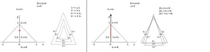
Figure 1: The types of deformations of the momentum triangle we are considering. Left: Conformal transformation of the triangle. In the $\gamma,\beta$ plane this corresponds to a constant (red) point. Right: Keeping the perimeter of the triangle $K$ constant we change the shape of an isosceles $\gamma=0$ triangle, moving along the bold red line for $k_{1}=k_{2}\geq k_{3}$.

3 Sources of scale dependence

3.1 Long-wavelength results

In this paper we use the long-wavelength formalism to study the parameter of non-Gaussianity $f_{\mathrm{NL}}$ and its scale dependence. The long-wavelength formalism consists of doing a perturbative expansion of the exact differential equations for the non-linear cosmological perturbations on super-horizon scales, which were obtained by neglecting second-order spatial gradient terms (see [35, 11, 20]). Slow-roll solutions for the first-order perturbations at horizon-crossing are used as initial conditions. The super-horizon assumption is equivalent to the leading order of the spatial gradient expansion and requires the slow-roll assumption to be satisfied at horizon-crossing (but not afterwards, see [40, 41, 20]). The non-Gaussianity parameter for an isosceles triangle of the form $k_{1}=k_{2}\equiv k^{\prime}\geq k_{3}\equiv k$ was found in [20] to be

$$-\frac{6}{5}f_{\mathrm{NL}}=\frac{-2{\bar{v}}_{12k^{\prime}}/[1+({\bar{v}}_{12k^{\prime}})^{2}]}{1+({\bar{v}}_{12k^{\prime}})^{2}+2\frac{\gamma_{k}^{2}}{\gamma_{k}^{\prime 2}}[1+({\bar{v}}_{12k})^{2}]}\! \!\!\Bigg{[} \!\!{\bar{v}}_{12k^{\prime}}\!\Bigg{(}\!g_{sr}(k^{\prime},k^{\prime})\!+\!g_{iso}(k^{\prime},k^{\prime})\!+\!g_{int}(k^{\prime},k^{\prime})\!\Bigg{)}$$ (3.1)

$$+2\frac{\gamma_{k}^{2}}{\gamma_{k}^{\prime 2}}{\bar{v}}_{12k}\Bigg{(}g_{sr}(k^{\prime},k)\!+\!g_{iso}(k^{\prime},k)\!+\!g_{int}(k^{\prime},k)\!\Bigg{)}\Bigg{]},$$

where $f_{\mathrm{NL}}=f_{\mathrm{NL}}(t;t_{k^{\prime}},t_{k})$ depends on $t_{k^{\prime}}$ and $t_{k}$, denoting the horizon-crossing times of the two scales $k^{\prime}$ and $k$ of the triangle, respectively. This result is exact and valid beyond the slow-roll approximation after horizon-crossing. All quantities appearing in this formula will be explained below.

The quantity ${\bar{v}}_{12}$ is a transfer function showing how the isocurvature mode (denoted by the subscript $2$) sources the adiabatic component $\zeta_{1}$. In the following two more transfer functions will appear, namely ${\bar{v}}_{22}$ and ${\bar{v}}_{32}$, showing how the isocurvature mode sources the isocurvature component $\zeta_{2}$ and the velocity of the isocurvature component $\theta_{2}\equiv\dot{\zeta_{2}}$, respectively. ${\bar{v}}_{a2}$ is a function of the horizon-exit time $t_{k}$ of the relevant perturbation of scale $k$ and it also evolves with time $t$, at least during inflation. In (3.1) as well as in the formulas that follow, ${\bar{v}}_{a2k}\equiv{\bar{v}}_{a2}(t,t_{k})$. The indices $a,b$ take the values $1,2,3$, indicating respectively the adiabatic perturbation $\zeta_{1}$, the isocurvature perturbation $\zeta_{2}$, and the isocurvature velocity $\theta_{2}$. ${\bar{v}}_{a2}$ comes from the combination of the Green’s functions $G_{a2}$ and $G_{a3}$ of the system of equations for the super-horizon perturbations (for the system of equations that the Green’s functions obey see [11, 20]):

$${\bar{v}}_{a2}(t,t_{k})=G_{a2}(t,t_{k})-\chi_{k}G_{a3}(t,t_{k}).$$ (3.2)

The quantity $\gamma_{k}$ in (3.1) is defined as $\gamma_{k}\equiv-\kappa H_{k}/(2k^{3/2}\sqrt{\epsilon_{k}})$ (and is not related to the $\gamma$ defined in (2.10)).

Except for the overall factor, $f_{\mathrm{NL}}$ has been split into three contributions: $g_{sr}$, $g_{iso}$ and $g_{int}$. $g_{sr}$ is a term that is slow-roll suppressed, since it depends only on horizon-exit quantities, where by assumption slow-roll holds,

$$g_{sr}({k}_{1},{k}_{2}) = \eta^{\perp}_{k_{1}}\Bigg{(}\frac{G_{22k_{1}k_{2}}{\bar{v}}_{12k_{1}}}{2}-\frac{1}{{\bar{v}}_{12k_{2}}}-\frac{G_{22k_{1}k_{2}}}{2{\bar{v}}_{12k_{1}}}\Bigg{)}+\frac{3\chi_{k_{2}}}{4}G_{33k_{1}k_{2}}-\frac{3}{2}(\epsilon_{k_{1}}+\eta^{\parallel}_{k_{1}})G_{22k_{1}k_{2}}$$ (3.3)

$$+\frac{\chi_{k_{1}}}{4}\Bigg{(}2\frac{{\bar{v}}_{12k_{1}}}{{\bar{v}}_{12k_{2}}}+G_{22k_{1}k_{2}}\Bigg{)}-\frac{\epsilon_{k_{1}}+\eta^{\parallel}_{k_{1}}}{2(\widetilde{v}_{12})^{2}}$$

$$+\frac{G_{13}(t,t_{k_{1}})}{2}\Bigg{[}\frac{3\left(\chi_{k_{1}}G_{22k_{1}k_{2}}-\chi_{k_{2}}G_{33k_{1}k_{2}}\right)}{2{\bar{v}}_{12k_{1}}}+G_{32k_{1}k_{2}}\left(\frac{3+\epsilon_{k_{1}}+2\eta^{\parallel}_{k_{1}}}{2{\bar{v}}_{12k_{1}}}+\eta^{\perp}_{k_{1}}\right)\Bigg{]}$$

$$-\frac{3}{4}G_{32k_{1}k_{2}}-\frac{1}{2}G_{12k_{1}k_{2}}\left(\epsilon_{k_{1}}+\eta^{\parallel}_{k_{1}}+2\eta^{\perp}_{k_{1}}-\frac{\chi_{k_{1}}}{2}\left(1+{\bar{v}}_{12k_{1}}\right)+\frac{\epsilon_{k_{1}}+\eta^{\parallel}_{k_{1}}}{{\bar{v}}_{12k_{1}}}\right).$$

Here we introduce some new notation,

$$\begin{array}[]{l}(\widetilde{v}_{12})^{2}\equiv{\bar{v}}_{12k_{1}}{\bar{v}}_{12k_{2}},\qquad(\widetilde{v}_{22})^{2}\equiv{\bar{v}}_{22k_{1}}{\bar{v}}_{22k_{2}},\qquad(\widetilde{v}_{32})^{2}\equiv{\bar{v}}_{32k_{1}}{\bar{v}}_{32k_{2}},\\ \widetilde{v}_{22}\widetilde{v}_{32}\equiv\frac{1}{2}({\bar{v}}_{22k_{1}}{\bar{v}}_{32k_{2}}+{\bar{v}}_{22k_{2}}{\bar{v}}_{32k_{1}}),\end{array}$$

and also $G_{abk_{1}k_{2}}\equiv G_{ab}(t_{k_{1}},t_{k_{2}})$. Moreover, we assume $k_{1}\geq k_{2}$. $g_{sr}$ is the only term from which a (small) part survives in the single-field limit, i.e.  in the limit where ${\bar{v}}_{12}=0$ at all times. For the equilateral case $k^{\prime}=k$ the two last lines of $g_{sr}$ are zero, since the Green’s functions satisfy

$$G_{ab}(t,t)=\delta_{ab}.$$ (3.4)

The contribution $g_{iso}$ is a term that survives as long as the isocurvature modes are alive,

$$g_{iso}({k}_{1},{k}_{2})=(\epsilon+\eta^{\parallel})(\widetilde{v}_{22})^{2}+\widetilde{v}_{22}\widetilde{v}_{32}.$$ (3.5)

If at the end of inflation these are non-zero, $f_{\mathrm{NL}}$ can still evolve afterwards and we cannot be sure that its value survives until today. Finally, $g_{int}$ is given by

$$g_{int}({k}_{1},{k}_{2})=\!-\!\int_{t_{k_{1}}}^{t}\!\!\!\!\mathrm{d}t^{\prime}\Big{[}2(\eta^{\perp})^{2}(\widetilde{v}_{22})^{2}\!+\!(\epsilon+\eta^{\parallel})\widetilde{v}_{22}\widetilde{v}_{32}\!+\!(\widetilde{v}_{32})^{2}\!-\!G_{13}(t,t^{\prime})\widetilde{v}_{22}(C\widetilde{v}_{22}+9\eta^{\perp}\widetilde{v}_{32})\Big{]}$$ (3.6)

with

$$C\equiv 12\eta^{\perp}\chi-6\eta^{\parallel}\eta^{\perp}+6(\eta^{\parallel})^{2}\eta^{\perp}+6(\eta^{\perp})^{3}-2\eta^{\perp}\xi^{\parallel}-2\eta^{\parallel}\xi^{\perp}-\sqrt{\frac{\epsilon}{2}}\frac{1}{\kappa H^{2}}(W_{211}+W_{222}),$$ (3.7)

where $W_{mnl}=W^{,ABC}e_{mA}e_{nB}e_{lC}$. It is from this integrated effect that any large, persistent non-Gaussianity originates, if we consider only models where the isocurvature modes have vanished by the end of inflation. For the analytical approximations that we will provide (in addition to the exact numerical results), it is useful to note that within the slow-roll approximation $g_{int}$ can be rewritten as

$$g_{int}(k_{1},k_{2})={\bar{v}}_{12k_{1}}G_{22k_{1}k_{2}}\left(-\eta^{\perp}_{k_{1}}+\frac{(\epsilon_{k_{1}}+\eta^{\parallel}_{k_{1}}-\chi_{k_{1}})\chi_{k_{1}}}{2\eta^{\perp}_{k_{1}}}\right)+{\tilde{g}}_{int}(k_{1},k_{2}),$$ (3.8)

where ${\tilde{g}}_{int}$ is another integral that is identically zero for the two-field quadratic model, or even more generally for any two-field equal-power sum model (see [20] for details).

3.2 Discussion

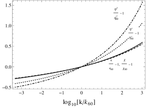
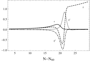
Figure 2: Left: The relative change of the horizon-crossing first-order slow-roll parameters $\epsilon$ (solid curve), $\eta^{\parallel}$ (dot-dashed curve), $\eta^{\perp}$ (dotted curve) and $\chi$ (dashed curve) at $t_{k}$ as a function of the ratio $k/k_{60}$ of the horizon-exit scale to the scale that left the horizon $60$ e-folds before the end of inflation, for the model (3.9) with mass ratio $m_{\phi}/m_{\sigma}=9$. Right: The evolution of the first-order slow-roll parameters $\epsilon$ (solid curve), $\eta^{\parallel}$ (dot-dashed curve), $\eta^{\perp}$ (dotted curve) and $\chi$ (dashed curve) as a function of the number of e-foldings $N-N_{60}$ for the time interval around the turning of the fields, for the same model.

Inspecting (3.1) ones sees that there are two sources of momentum dependence for $f_{\mathrm{NL}}$: the slow-roll parameters at horizon-crossing and the Green’s functions $G_{ab}$ or their combinations ${\bar{v}}_{a2}$. In order to study their impact we shall use the quadratic model

$$W=\frac{1}{2}m_{\phi}^{2}\phi^{2}+\frac{1}{2}m_{\sigma}^{2}\sigma^{2},$$ (3.9)

with $m_{\phi}/m_{\sigma}=9$. The procedure to follow is to solve for the background quantities (2.4) and then for the Green’s functions (see subsection 2.2 in [20]) in order to apply the formalism. The quadratic model’s Green’s functions can be found numerically, or even analytically within the slow-roll approximation, which is valid for a small mass ratio like the one we chose here. However, all our calculations in this paper are numerical and exact, without assuming the slow-roll approximation after horizon crossing. We only use the slow-roll approximation after horizon crossing for the analytical approximations that we provide (e.g. eq. (4.1)) and sometimes to clarify the physical interpretation of results (e.g. the use of (3.11) below to explain the behaviour of ${\bar{v}}_{12}$). Inflation ends at $t_{f}$ defined as the time when $\epsilon_{f}=1$. From now on a subscript $f$ will denote quantities evaluated at the end of inflation. We also define the scale that exited the horizon $60$ e-folds before the end of inflation as $k_{60}$ and use it as a reference scale, around which we perform our computations ($k_{60}$ being the scale that corresponds to the text books’ minimal necessary amount of inflation).

In figure 2 we plot the first-order slow-roll parameters for a range of horizon-crossing times around $k_{60}$. While the heavy field rolls down its potential the slow-roll parameters increase, reflecting the evolution of the background. This implies that $f_{\mathrm{NL}}$, which is in general proportional to the slow-roll parameters evaluated at $t_{k}$ and $t_{k^{\prime}}$, should increase as a function of $k$ and $k^{\prime}$. This can easily be verified for the initial value of $f_{\mathrm{NL},in}$ at $t=t_{k^{\prime}}$, which according to (3.1) with ${\bar{v}}_{12k^{\prime}}=0$ takes the value

$$-\frac{6}{5}f_{\mathrm{NL},in}=\epsilon_{k^{\prime}}+\eta^{\parallel}_{k^{\prime}}+\frac{2\frac{\gamma_{k}^{2}}{\gamma^{2}_{k^{\prime}}}G_{12k^{\prime}k}}{1+2\frac{\gamma_{k}^{2}}{\gamma^{2}_{k^{\prime}}}[1+(G_{12k^{\prime}k})^{2}]}\eta^{\perp}_{k^{\prime}}G_{22k^{\prime}k}.$$ (3.10)

Figure 3: The evolution of the transfer functions ${\bar{v}}_{12}$ (left) and ${\bar{v}}_{22}$ (right) as a function of the number of e-foldings $N-N_{60}$ for the time interval around the turning of the fields and for different horizon exit scales, varying from top to bottom as $k_{60}\times 10$ (dotted curve), $k_{60}$ (solid curve) and $k_{60}/10$ (dashed curve), for the model (3.9) with mass ratio $m_{\phi}/m_{\sigma}=9$.

Apart from the slow-roll parameters the other source of momentum dependence for $f_{\mathrm{NL}}$ lies in the Green’s functions and particularly how their time evolution depends on the relevant horizon-crossing scale. The two main quantities that we need to study in order to understand their impact on $f_{\mathrm{NL}}$ are the transfer functions ${\bar{v}}_{12}$ and ${\bar{v}}_{22}$. This is due to the fact that ${\bar{v}}_{32}$ is slow-roll suppressed and the rest of the Green’s functions appearing in (3.1) can be rewritten in terms of ${\bar{v}}_{12}$ and ${\bar{v}}_{22}$ within the slow-roll approximation (for details, see [20]). In particular $G_{a3}=G_{a2}/3$, $G_{32}(t,t_{k})=-\chi(t)G_{22}(t,t_{k})$ and hence $G_{a2}\approx{\bar{v}}_{a2}$. Note that except for the era of the turning of the fields, the slow-roll assumption is a good approximation during inflation in this particular model. The slow-roll evolution equations for ${\bar{v}}_{12k}$ and ${\bar{v}}_{22k}$ are

$$\frac{\mathrm{d}}{\mathrm{d}t}{\bar{v}}_{12k}=2\eta^{\perp}{\bar{v}}_{22k}\qquad\mathrm{and}\qquad\frac{\mathrm{d}}{\mathrm{d}t}{\bar{v}}_{22k}=-\chi{\bar{v}}_{22k}.$$ (3.11)

As was discussed above, ${\bar{v}}_{12}$ describes how the isocurvature mode sources the adiabatic one, while ${\bar{v}}_{22}$ describes how the isocurvature mode sources itself. By definition ${\bar{v}}_{12}(t_{k},t_{k})=0$ and ${\bar{v}}_{22}(t_{k},t_{k})=1$ at horizon crossing, since no interaction of the different modes has yet occurred (see also (3.2) and (3.4)). For the transfer functions of the adiabatic mode one finds that ${\bar{v}}_{11}=1$ and ${\bar{v}}_{21}=0$, since the curvature perturbation is conserved for purely adiabatic perturbations and adiabatic perturbations cannot source entropy perturbations. In order to better understand the role of the transfer functions, we can use the Fourier transformation of the perturbations [20] along with these last identities, to find

$$\zeta_{1}(t)=\int\frac{\mathrm{d}^{3}{\boldsymbol{k}}}{(2\pi)^{3/2}}\gamma_{k}{\bar{v}}_{1m}\hat{a}^{\dagger}_{m}({\boldsymbol{k}})e^{\mathrm{i}{\boldsymbol{k}}\cdot{\boldsymbol{x}}}=\zeta_{1}(t_{k})+{\bar{v}}_{12}(t,t_{k})\zeta_{2}(t_{k}),$$

$$\zeta_{2}(t)=\int\frac{\mathrm{d}^{3}{\boldsymbol{k}}}{(2\pi)^{3/2}}\gamma_{k}{\bar{v}}_{2m}\hat{a}^{\dagger}_{m}({\boldsymbol{k}})e^{\mathrm{i}{\boldsymbol{k}}\cdot{\boldsymbol{x}}}={\bar{v}}_{22}(t,t_{k})\zeta_{2}(t_{k}),$$ (3.12)

where $\zeta_{m}$ with $m=1,2$ are the first-order adiabatic and isocurvature perturbation.

Let us start by discussing the time evolution of ${\bar{v}}_{12}$. Each one of the curves on the left-hand side of figure 3 corresponds to the time evolution of ${\bar{v}}_{12}$ for a different horizon-exit scale. At $t=t_{k}$, i.e.  when the relevant mode $k$ exits the horizon, ${\bar{v}}_{12k}=0$ since the isocurvature mode has not had time to affect the adiabatic one. Outside the horizon and well in the slow-roll regime of the sole dominance of the heavy field, the isocurvature mode sources the adiabatic one and the latter slowly increases. As time goes by, the heavy field rolls down its potential and the light field becomes more important. During this turning of the field trajectory, the slow-roll parameters suddenly change rapidly, with important consequences for the evolution of the adiabatic and isocurvature mode. The transfer function ${\bar{v}}_{12k}$ grows substantially during that era because of the increasing values of $\eta^{\perp}$ in (3.11) as well as the growing contribution of ${\bar{v}}_{22k}$, to become constant afterwards when the light field becomes dominant in an effectively single-field universe.

Note that the earlier the mode exits the horizon, the smaller is the final ${\bar{v}}_{12k}$. This is opposite to the behaviour of the initial value, just after horizon-crossing, when the earlier the scale exits the horizon the more has its adiabatic mode been sourced by the isocurvature one at a given time $t$, and hence the larger is its ${\bar{v}}_{12k}$. This can be understood by the evolution equations of ${\bar{v}}_{12k}$ and ${\bar{v}}_{22k}$ in (3.11), showing that ${\bar{v}}_{12k}$ is sourced by ${\bar{v}}_{22k}$, which itself is a decreasing function of time, at least during eras when the universe is dominated by a single field (see the right-hand side of figure 3). If the equation (3.11) for ${\bar{v}}_{12k}$ did not depend on $\eta^{\perp}$, the ${\bar{v}}_{12k}$ curves would never cross each other since they would be similar and only boosted by their horizon-crossing time shift. It is the increasing value of $\eta^{\perp}$ that results in the larger values of ${\bar{v}}_{12k}$ for larger $k$.

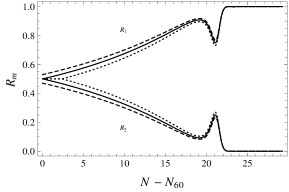
Figure 4: Left: The time evolution of the adiabatic $R_{1}$ and the isocurvature $R_{2}$ ratios of power spectra as a function of the number of e-foldings $N-N_{60}$ for scales $k_{60}/10$ (dashed line), $k_{60}$ (solid line) and $k_{60}\times 10$ (dotted line). Right: The time evolution of the spectral index (2.2) as a function of the number of e-foldings $N-N_{60}$ for scales $k_{60}/10$ (dashed line), $k_{60}$ (solid line) and $k_{60}\times 10$ (dotted line). Both plots are made for the model (3.9) with mass ratio $m_{\phi}/m_{\sigma}=9$.

On the right-hand side of figure 3 we show the evolution of ${\bar{v}}_{22}$. According to (3.11) ${\bar{v}}_{22}$ and hence the isocurvature mode evolves independently from the adiabatic mode. At horizon-crossing $t=t_{k}$, the transfer function ${\bar{v}}_{22k}=1$. Once outside the horizon, the isocurvature mode decays due to the small but positive values of $\chi$. During the turning of the fields the slow-roll parameters evolve rapidly, thus leading to first an enhancement of ${\bar{v}}_{22k}$ and then a diminution due to the varying value of $\chi$ in (3.11). As can be seen from the right-hand side plot in figure 2, during the turning $\chi$ first becomes negative and then positive. After the turning of the fields, the remnant isocurvature modes again decay and (for this model) at the end of inflation none are left. The parameter $\chi$ plays a crucial role in the evolution of the isocurvature mode. It represents effectively the second derivative of the potential in the $22$ direction. Before the turning of the fields the trajectory goes down the potential in the relatively steep $\phi$ direction, which means that $W_{22}$ then corresponds with the relatively shallow curvature in the direction of the light field $\sigma$ and hence $\chi$ is small. After the turning the trajectory goes along the bottom of the valley in the $\sigma$ direction and $W_{22}$ corresponds with the large curvature of the potential in the perpendicular direction, leading to large values of $\chi$. The negative values of $\chi$ during the turn come from the contribution of $\eta^{\parallel}$.

Instead of looking at the tranfer functions, using (3.12) one can also construct more physical quantities from the operators $\zeta_{m}$ and hence from the ${\bar{v}}_{m2}$, namely the ratios of the adiabatic and isocurvature power spectrum to the total power spectrum:

$$R_{1}\equiv\frac{\langle\zeta_{1}\zeta_{1}\rangle}{\langle\zeta_{1}\zeta_{1}\rangle+\langle\zeta_{2}\zeta_{2}\rangle}=\frac{1+\left({\bar{v}}_{12}\right)^{2}}{1+\left({\bar{v}}_{12}\right)^{2}+\left({\bar{v}}_{22}\right)^{2}},$$

$$R_{2}\equiv\frac{\langle\zeta_{2}\zeta_{2}\rangle}{\langle\zeta_{1}\zeta_{1}\rangle+\langle\zeta_{2}\zeta_{2}\rangle}=\frac{\left({\bar{v}}_{22}\right)^{2}}{1+\left({\bar{v}}_{12}\right)^{2}+\left({\bar{v}}_{22}\right)^{2}}.$$ (3.13)

These are plotted on the left-hand side of figure 4 as a function of the number of e-foldings for different scales. One can clearly see that both ratios start as equal to $1/2$ when the scale exits the horizon, while afterwards the adiabatic ratio $R_{1}$ increases to reach $1$ at the end of inflation and the isocurvature $R_{2}$ decreases to reach $0$, for this particular model. During the turning of the fields we see that the temporary increase in the isocurvature mode due to the negative value of $\chi$ is reflected in $R_{2}$, while the adiabatic $R_{1}$ necessarily has the opposite behaviour.

On the right-hand side of figure 4 we plot the time evolution of the spectral index (2.2) of the power spectrum. The spectral index measures by construction the tilt of the power spectrum for different horizon-crossing scales and hence it depends on the horizon-crossing slow-roll parameters. For multiple-field models the power spectrum evolves during inflation even after horizon-crossing, and so does the spectral index. During the turning of the fields the spectral index increases, to remain constant afterwards. The earlier a scale exits the horizon the less negative is its spectral index $n_{\zeta}-1$. This implies that the power spectrum itself decreases faster for larger horizon-crossing scales. This is due to the fact that except for the factor $1+({\bar{v}}_{12k})^{2}$ in the expression for the power spectrum there is also an inverse power of $\epsilon_{k}$ (see [20]).

3.3 Spectral indices

Finally let us discuss the scale dependence of the local $f_{\mathrm{NL}}$ in terms of the relevant spectral indices. Equation (3.1) for an isosceles triangle implies that

$$-\frac{6}{5}f_{\mathrm{NL}} = \frac{1}{(2\pi^{2})^{2}}\frac{f(k^{\prime},k^{\prime})+2(\frac{k^{\prime}}{k})^{3}f(k^{\prime},k)}{\mathcal{P}_{\zeta}(k^{\prime})^{2}+2(\frac{k^{\prime}}{k})^{3}\mathcal{P}_{\zeta}(k^{\prime})\mathcal{P}_{\zeta}(k)},$$ (3.14)

where

$$f(k^{\prime},k)=-2(k^{\prime}k)^{3}\gamma_{k^{\prime}}^{2}\gamma_{k}^{2}\,{\bar{v}}_{12k^{\prime}}{\bar{v}}_{12k}\left(g_{sr}(k^{\prime},k)+g_{iso}(k^{\prime},k)+g_{int}(k^{\prime},k)\right).$$ (3.15)

For an arbitrary triangle configuration this is generalized as

$$-\frac{6}{5}f_{\mathrm{NL}} = \frac{1}{(2\pi^{2})^{2}}\frac{k_{3}^{3}f(k_{1},k_{2})+\mathrm{perms.}}{k_{3}^{3}\mathcal{P}_{\zeta}(k_{1})\mathcal{P}_{\zeta}(k_{2})+\mathrm{perms.}}.$$ (3.16)

The local $f_{\mathrm{NL}}$ depends on a two-variable function $f(k_{1},k_{2})$, with $k_{1}\geq k_{2}$. This is due to its super-horizon origin, which yields classical non-Gaussianity proportional to products of two power spectra. Hence one expects that the scale dependence of $f_{\mathrm{NL}}$ can be expressed in terms of only two spectral indices, characterizing the function $f$. Notice that this is particular to the local case. In general the bispectrum cannot be split as a sum of two-variable functions and one anticipates that three spectral indices would be needed.

The next issue to be resolved is which are the relevant spectral indices for $f$. The naive guess would be $f(k_{1},k_{2})=f(k_{1,0},k_{2,0})(k_{1}/k_{1,0})^{{\tilde{n}}_{k_{1}}}(k_{2}/k_{2,0})^{{\tilde{n}}_{k_{2}}}$. We tested this parametrization and we did not find good agreement with the exact value of $f$. Instead of that, we found that $f$ is best approximated by keeping either the shape or the magnitude of the triangle constant. This statement can be expressed as

$$f(k_{1},k_{2})=f_{0}\left(\frac{K}{K_{0}}\right)^{{\tilde{n}}_{K}}\left(\frac{\omega}{\omega_{0}}\right)^{{\tilde{n}}_{\omega}},$$ (3.17)

where

$${\tilde{n}}_{K}\equiv\frac{\mathrm{d}\ln f}{\mathrm{d}\ln K}\qquad\mathrm{and}\qquad{\tilde{n}}_{\omega}\equiv\frac{\mathrm{d}\ln f}{\mathrm{d}\ln\omega}$$ (3.18)

and

$$\omega\equiv\frac{k_{1}}{k_{2}}=\frac{1+\beta}{2(1-\beta)}.$$ (3.19)

The last equality is valid only for the isosceles case $\gamma=0$ (see (2.10)). We dropped the $-1$ of the power spectrum spectral index definition to follow the definitions in [33, 32]. We added a tilde to indicate that these spectral indices are defined for the function $f$, not yet for the full $f_{\mathrm{NL}}$. In the next two sections we are going to examine the scale-dependence of $f_{\mathrm{NL}}$, changing the magnitude and the shape of the triangle separately, and verify assumption (3.17).

4 Changing the magnitude of the triangle

Figure 5: The time evolution of $f_{\mathrm{NL}}$ in terms of the number of e-foldings $N-N_{60}$ around the time of the turning of the fields, for equilateral ($\omega=1$) triangles with $K=(3/2)k_{60}$ (solid curve), $K=(3/2)k_{60}/10$ (dashed curve) and $K=(3/2)k_{60}\times 10$ (dotted curve), for the model (3.9) with mass ratio $m_{\phi}/m_{\sigma}=9$.

In this section we shall study the behaviour of $f_{\mathrm{NL}}$ for triangles of the same shape but different size, see the left-hand side of figure 1. In figure 5 we plot the time evolution of $f_{\mathrm{NL}}$ for equilateral triangles (the result would remain qualitatively the same for any isosceles triangle) of perimeter $K=(3/2)k_{60}\times 10$ (top curve), $K=(3/2)k_{60}$ (middle curve) and $K=(3/2)k_{60}/10$ (bottom curve). The later the relevant scale exits the horizon the larger is its initial $f_{\mathrm{NL}}$ as explained in the previous section. $f_{\mathrm{NL}}$ grows during the turning of the fields due to isocurvature effects as described by (3.5) and (3.6), but by the end of inflation, when isocurvature modes vanish, it relaxes to a small, slow-roll suppressed value (see e.g.  [19, 20]). In figure 6 we plot the final value of $f_{\mathrm{NL}}$ (left) and the final value of the bispectrum (right) for equilateral triangles, varying $K$ for values around $K=(3/2)k_{60}$, within the Planck satellite’s resolution ($k^{\prime}/k\sim 1000$). The later the scale exits the horizon, i.e.  the larger $K$, the larger is the final value of $f_{\mathrm{NL}}$ and of the bispectrum.

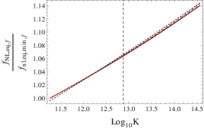
Figure 6: Left: The relative change of the final value of $f_{\mathrm{NL}}$ arbitrarily normalized to one at the smallest value of $K$ on the figure, as a function of $K$ for equilateral triangles ($\omega=1$), calculated exactly (solid curve), using the analytical approximation (4.1) (dashed red curve) and using the shape index (4.6) (dotted black curve). Right: The logarithm of the final value of the exact bispectrum, similarly normalized, as a function of $K$ for equilateral triangles ($\omega=1$). Both figures are for the quadratic model (3.9) with mass ratio $m_{\phi}/m_{\sigma}=9$. The vertical dashed line corresponds to $K=(3/2)k_{60}$.

The final value of $f_{\mathrm{NL}}$ can be found analytically for the quadratic model within the slow-roll approximation. By the end of inflation ${\bar{v}}_{22,f}=0$ so that (3.5) vanishes, while (3.6) can be further simplified to give some extra horizon-crossing terms and a new integral ${\tilde{g}}_{int}$ that is identically zero for the quadratic potential (see (3.8) and [20]). For simplicity we give here the final value of $f_{\mathrm{NL}}$ for equilateral triangles,

$$f_{\mathrm{NL},eq,f}(k)=\frac{3\left({\bar{v}}_{12k}\right)^{2}\left(\epsilon_{k}+\eta^{\parallel}_{k}-\chi_{k}+\frac{\eta^{\perp}_{k}}{{\bar{v}}_{12k}}\right)+\left({\bar{v}}_{12k}\right)^{3}\left(\eta^{\perp}_{k}-\frac{\left(\epsilon_{k}+\eta^{\parallel}_{k}-\chi_{k}\right)\chi_{k}}{\eta^{\perp}_{k}}\right)+\epsilon_{k}+\eta^{\parallel}_{k}}{\left(1+\left({\bar{v}}_{12k}\right)^{2}\right)^{2}}.$$ (4.1)

This formula is actually valid for any two-field model for which isocurvature modes vanish at the end of inflation and for which ${\tilde{g}}_{int}=0$, like for example equal-power sum models. Inspecting the various terms it turns out that although ${\bar{v}}_{12k}$ tends to decrease the value of $f_{\mathrm{NL},f}$ as a function of $k$, it is the contribution of the horizon-crossing slow-roll parameters that wins and leads to an increase of the parameter of non-Gaussianity for larger horizon-crossing scales. Note that for equilateral triangles $K$ is simply $3k/2$.

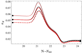
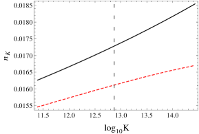
Figure 7: Left: The time evolution of the conformal index $n_{K}$ (4.2) around the time of the turning of the fields, for triangles with $\omega=1$ (black curves) and $\omega=5/2$ (red curves, below the $\omega=1$ curves), with perimeter $K=(3/2)k_{60}$ (solid curve), $K=(3/2)k_{60}/10$ (dashed curve) and $K=(3/2)k_{60}\times 10$ (dotted curve). The three points on the left and on the right correspond to the analytical values of the index as calculated from (4.7) and (A.1) respectively. Right: The final value of the conformal index $n_{K}$ (4.2) for triangles with $\omega=1$ (black curve) and $\omega=5/2$ (red dashed curve) as a function of $K$. Both figures are for the model (3.9) with mass ratio $m_{\phi}/m_{\sigma}=9$.

We turn now to the spectral index $n_{K}$. Using (3.18) with (2.11) and assuming that $\gamma=0$ and $\beta=\mathrm{const.}$, we can express ${\tilde{n}}_{K}$ in terms of the horizon-crossing time derivatives as

$${\tilde{n}}_{K}(t;t_{k_{1}},t_{k_{2}})=\frac{\partial\ln{f}}{\partial t_{k_{1}}}\frac{1}{1-\epsilon_{k_{1}}}+\frac{\partial\ln{f}}{\partial t_{k_{2}}}\frac{1}{1-\epsilon_{k_{2}}}.$$ (4.2)

Then $f_{\mathrm{NL}}$ takes the form

$$-\frac{6}{5}f_{\mathrm{NL}}=\frac{1}{(2\pi^{2})^{2}}\frac{f(k^{\prime}_{0},k^{\prime}_{0})\left(\frac{K}{K_{0}}\right)^{{\tilde{n}}_{K}(t_{k^{\prime}_{0}},t_{k^{\prime}_{0}})}+2\omega^{3}f(k^{\prime}_{0},k_{0})\left(\frac{K}{K_{0}}\right)^{{\tilde{n}}_{K}(t_{k^{\prime}_{0}},t_{k_{0}})}}{\mathcal{P}_{\zeta}(k^{\prime}_{0})^{2}\left(\frac{k^{\prime}}{k^{\prime}_{0}}\right)^{2(n_{\zeta}(t_{k^{\prime}_{0}})-1)}+2\omega^{3}\mathcal{P}_{\zeta}(k^{\prime}_{0})\mathcal{P}_{\zeta}(k_{0})\left(\frac{k^{\prime}}{k^{\prime}_{0}}\right)^{n_{\zeta}(t_{k^{\prime}_{0}})-1}\left(\frac{k}{k_{0}}\right)^{n_{\zeta}(t_{k_{0}})-1}}.$$ (4.3)

Note that the ratios $k^{\prime}/k^{\prime}_{0}=k/k_{0}=K/K_{0}$, since $\beta=\mathrm{const}$.

The above formula can be simplified in the limit of squeezed-triangle configurations, as well as in the equilateral limit. When one takes the squeezed limit $\omega^{3}\mg 1$ (note that this would be true for $\beta\gtrsim 2/3$), one finds:

$$-\frac{6}{5}f_{\mathrm{NL}} = \frac{1}{(2\pi^{2})^{2}}\frac{f(k^{\prime}_{0},k_{0})}{\mathcal{P}_{\zeta}(k^{\prime}_{0})\mathcal{P}_{\zeta}(k_{0})}\left(\frac{K}{K_{0}}\right)^{{\tilde{n}}_{K}(t_{k^{\prime}_{0}},t_{k_{0}})-n_{\zeta}(t_{k^{\prime}_{0}})-n_{\zeta}(t_{k_{0}})+2}$$ (4.4)

$$\equiv -\frac{6}{5}f_{\mathrm{NL},0}\left(\frac{K}{K_{0}}\right)^{n_{K}(t_{k^{\prime}_{0}},t_{k_{0}})},$$

where

$$n_{K}(t;t_{k^{\prime}},t_{k})\equiv\frac{\mathrm{d}\ln f_{\mathrm{NL}}}{\mathrm{d}\ln K}=\frac{\partial\ln{f_{\mathrm{NL}}}}{\partial t_{k^{\prime}}}\frac{1}{1-\epsilon_{k^{\prime}}}+\frac{\partial\ln{f_{\mathrm{NL}}}}{\partial t_{k}}\frac{1}{1-\epsilon_{k}}.$$ (4.5)

For the equilateral case $\omega=1$, (4.3) becomes

$$-\frac{6}{5}f_{\mathrm{NL}} = \frac{1}{(2\pi^{2})^{2}}\frac{f(k^{\prime}_{0},k^{\prime}_{0})}{\mathcal{P}_{\zeta}(k^{\prime}_{0})^{2}}\left(\frac{K}{K_{0}}\right)^{{\tilde{n}}_{K}(t_{k^{\prime}_{0}},t_{k^{\prime}_{0}})-2n_{\zeta}(t_{k^{\prime}_{0}})+2}$$ (4.6)

$$\equiv -\frac{6}{5}f_{\mathrm{NL},0}\left(\frac{K}{K_{0}}\right)^{n_{K}(t_{k^{\prime}_{0}},t_{k^{\prime}_{0}})}.$$

The conformal spectral index $n_{K}$ measures the change of $f_{\mathrm{NL}}$ due to the overall size of the triangle, namely due to a conformal transformation of the triangle. For an isosceles triangle this is conceptually sketched on the left-hand side of figure 1, but it can be generalized for any shape. $n_{K}$ coincides with the $n_{f_{\mathrm{NL}}}$ of [33, 32] and grossly speaking it describes the tilt of $f_{\mathrm{NL}}$ due to the pure evolution of the inflationary background (note that for an equilateral triangle this statement would be exact).

On the left-hand side of figure 7 we plot the time evolution of the conformal spectral index for an equilateral $\omega=1$ and an isosceles $\omega=5/2$ triangle that exited the horizon at three different times, namely for $K=(3/2)k_{60}$ (solid curve), $K=(3/2)k_{60}/10$ (dashed curve) and $K=(3/2)k_{60}\times 10$ (dotted curve). We plot the $\omega=5/2$ case only to demonstrate that the results remain qualitatively the same; we shall study the effect of different triangle shapes in the next section. The characteristic peaks that $n_{K}$ exhibits during the turning of the fields are inherited from the behaviour of $f_{\mathrm{NL}}$ at that time and it is a new feature that is absent in the time evolution of the power spectrum spectral index $n_{\zeta}-1$ (see the right-hand side of figure 4).

In the context of the long-wavelength formalism we are restricted to work with the slow-roll approximation at horizon exit, so that the slow-roll parameters at that time should be small and vary just a little. This should be reflected in the initial value of the spectral index, which should be $\mathcal{O}(\epsilon_{k^{\prime}})$. In another paper we will study models that do not necessarily satisfy this constraint, using the exact cubic action derived in [39] instead of the long-wavelength formalism. The earlier the scale exits, e.g.  the dashed curve, the smaller are the slow-roll parameters evaluated at horizon crossing and hence the smaller is the initial $n_{K}$. Indeed, using the definition (4.5) with (3.10) for the initial value of $f_{\mathrm{NL},in}$, we find for equilateral triangles

$$n_{K,in}=\frac{2\epsilon_{k}^{2}+3\epsilon_{k}\eta^{\parallel}_{k}+(\eta^{\perp}_{k})^{2}-(\eta^{\parallel}_{k})^{2}+\xi^{\parallel}_{k}}{\epsilon_{k}+\eta^{\parallel}_{k}},$$ (4.7)

which confirms the above statement.

We notice that the initial, horizon-crossing, differences between the values of $n_{K}$ for the different horizon-crossing scales mostly disappear by the end of inflation, after peaking during the turning of the fields. The final value of the spectral index is plotted on the right-hand side of figure 7 and is smaller than its initial value. It exhibits a small running of $\mathcal{O}(10\%)$ within the range of scales studied, inherited from the initial dispersion of its values at horizon-crossing. To verify that $n_{K}$ describes well the behaviour of $f_{\mathrm{NL}}$, we have plotted the approximation (4.6) in figure 6 where it can be compared with the exact result. We have also verified this for other inflationary models, including the potential

$$W=b_{0}-b_{2}\sigma^{2}+b_{4}\sigma^{4}+a_{2}\phi^{2},$$ (4.8)

studied in [20], able to produce $f_{\mathrm{NL}}$ of ${\mathcal{O}}(1)$. The final value of the spectral index in that model is two orders of magnitude smaller than the value for the quadratic model. This is related essentially to the fact that for the potential (4.8) the turning of the fields, and hence the slow-roll breaking, occurs near the end of inflation. This means that at the horizon-crossing times of the scales of the triangle, slow-roll parameters change very slowly and as a result the initial variation of $f_{\mathrm{NL}}$ is much smaller than the one for the quadratic potential. As a consequence, the final tilt of $f_{\mathrm{NL}}$ will be smaller.

In Appendix A one can find the analytical expression for the final value of the spectral index $n_{K}$, found by differentiating (4.1). Since the result is rather lengthy and does not give any further physical intuition, we moved it to the appendix.

5 Changing the shape of the triangle

Figure 8: The time evolution of $f_{\mathrm{NL}}$ as a function of the number of e-foldings $N-N_{60}$ around the time of the turning of the fields, for a triangle with $\omega=1$ (solid curve), $\omega=5/2$ (dotted curve) and $\omega=1000$ (dashed curve), all with fixed perimeter $K=3/2k_{60}$, for the model (3.9) with mass ratio $m_{\phi}/m_{\sigma}=9$.

After studying triangles with the same shape but varying size in the previous section, we now turn to the scale dependence of $f_{\mathrm{NL}}$ for triangles of the same perimeter but different shape, see the right-hand side of figure 1. In figure 8 we plot the time evolution of $f_{\mathrm{NL}}$ during inflation for an equilateral $\omega=1$ (solid curve), an isosceles $\omega=5/2$ (dotted curve) and a squeezed $\omega=1000$ (dashed curve) triangle, all of perimeter $K=(3/2)k_{60}$, as a function of the number of e-foldings. The profile of the time evolution of $f_{\mathrm{NL}}$ was discussed in the previous section. Here we are interested in the shape dependence of $f_{\mathrm{NL}}$.

Although it is during the peak that the variation of $f_{\mathrm{NL}}$ for different shapes is more prominent, its final value is also affected. On the left-hand side of figure 9 we plot the value of $f_{\mathrm{NL}}$ at the end of inflation for triangles of perimeter $K=(3/2)k_{60}$, normalised by its value for the equilateral case ($\omega=1$), as a function of $\omega$. The deviation of the values is small since it is related to horizon-exit slow-roll suppressed quantities. Within the long-wavelength formalism (or the $\delta N$ formalism) slow roll at horizon crossing is a requirement. Nevertheless, the important conclusion here is that $f_{\mathrm{NL}}$ decreases when the triangle becomes more squeezed. This can be attributed to the fact that the more squeezed is the triangle, the more the fluctuation $\zeta_{k}$ is frozen and behaves as part of the background when scale $k^{\prime}$ crosses the horizon. As a result the correlation between $k$ and $k^{\prime}$ becomes less and the resulting non-Gaussianity is smaller (see also the discussion below equation (5.1).)

An analytical formula can be found when applying the slow-roll approximation to expression (3.1) at the end of inflation, when isocurvature modes have vanished. We perform an integration by parts in the integral (see (3.8) and [20]; as before ${\tilde{g}}_{int}=0$). More precisely, assuming that we are really in the squeezed limit $k\ll k^{\prime}$, the ratio $\gamma_{k}^{2}/\gamma_{k^{\prime}}^{2}$ becomes very large and we can ignore the equilateral terms that depend only on $k^{\prime}$ and not also on $k$. We also assume that the decaying mode has vanished to simplify the expressions for the Green’s functions (see [20] and the discussion in section 3). $G_{12k^{\prime}k}$ can be set to zero as one can see in figure 3 (since it is basically equal to ${\bar{v}}_{12}$ and only involves times at the very left-hand side of the figure). Moreover, the same figure shows that ${\bar{v}}_{12k}/{\bar{v}}_{12k^{\prime}}\approx 1$ (in the formula these ratios are always multiplied by slow-roll parameters, so that the deviation from 1 would be like a second-order effect), so that we find in the end

$$f_{\mathrm{NL},sq,f} = G_{22k^{\prime}k}f_{\mathrm{NL},eq,f}(k^{\prime})+\frac{1-G_{22k^{\prime}k}}{\left(1+\left({\bar{v}}_{12k^{\prime}}\right)^{2}\right)^{2}}\Bigg{[}\epsilon_{k^{\prime}}+\eta^{\parallel}_{k^{\prime}}+\left(\frac{2\eta^{\perp}_{k^{\prime}}}{{\bar{v}}_{12k^{\prime}}}-\chi_{k^{\prime}}\right)\left({\bar{v}}_{12k^{\prime}}\right)^{2}\Bigg{]},$$ (5.1)

where $f_{\mathrm{NL},eq,f}$ is given in equation (4.1). The only quantity in the above expression that depends on the shape of the triangle is $G_{22k^{\prime}k}$, so it must be $G_{22k^{\prime}k}$ that is responsible for the decreasing behaviour of $f_{\mathrm{NL},sq,f}$. Indeed, increasing $\omega$ for a constant perimeter $K$ of the triangle means increasing the interval $t_{k}-t_{k^{\prime}}$ and hence decreasing the value of $G_{22k^{\prime}k}$ (see the right-hand side of figure 3, since in the slow-roll regime ${\bar{v}}_{22}=G_{22}$). This means that the interaction of the two modes becomes less important. In the complete absence of isocurvature modes $G_{22k^{\prime}k}=0$ and $f_{\mathrm{NL},sq,f}$ takes its minimal value. It is only the isocurvature mode that interacts with itself and the greater is the difference between the two momenta the less is the interaction. Notice that the single-field limit of this result would correspond to $G_{22k^{\prime}k}=0$ and ${\bar{v}}_{12}=0$.

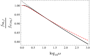
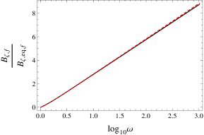
Figure 9: Left: The final value of $f_{\mathrm{NL}}$ normalised by the equilateral $f_{\mathrm{NL}}$ as a function of $\omega$ for triangles with $K=(3/2)k_{60}$ calculated exactly (black curve), using the analytical approximation (5.1) (dashed red curve) and using the shape index (5.4) (dotted black curve). Right: The logarithm of the final value of the exact local bispectrum normalised by the local bispectrum computed on an equilateral triangle as a function of $\omega$ for triangles with $K=(3/2)k_{60}$ (black curve) and the same quantity assuming $f_{\mathrm{NL}}$ scale independent (red dashed curve). Both figures are for the quadratic model (3.9) with mass ratio $m_{\phi}/m_{\sigma}=9$.

The decrease of $f_{\mathrm{NL}}$ for more squeezed triangles seems contradictory to the well-known fact that the local bispectrum is maximized for squeezed configurations. In order to clarify this subtle point, we stress that the left-hand side of figure 9 is essentially the ratio of the exact bispectrum to the bispectrum assuming $f_{\mathrm{NL}}$ as a constant (2.9) and hence the products of the power spectrum cancel out. We also plot on the right-hand side of figure 9 the final value of the bispectrum (2.9), normalised by the value of the bispectrum for equilateral triangles with $K=3k_{60}/2$. Although $f_{\mathrm{NL}}$ is maximal for equilateral triangles, the bispectrum has the opposite behaviour, since it is dominated by the contribution of the products of the power spectrum, which leads to an increased bispectrum for the more squeezed shape. At the same time though we show that there is a small contribution of $f_{\mathrm{NL}}$ itself, leading to smaller values of the bispectrum when compared to a bispectrum where $f_{\mathrm{NL}}$ is assumed to be constant.

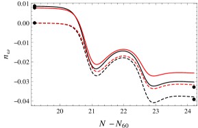
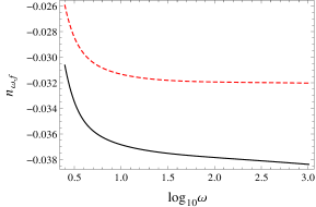
Figure 10: Left: The time evolution of the shape index $n_{\omega}$ (5.5) around the time of the turning of the fields, for constant $K=(3/2)k_{60}$ (black curves) and $K=(3/2)k_{60}/10$ (red curves, above the $K=(3/2)k_{60}$ curves), and for the shapes $\omega=5/2$ (solid curve) and $\omega=1000$ (dashed curve). The points on the left correspond to the analytical values of the index as calculated from (5.6), while the points on the right correspond to the values of the index as calculated from (A.2) for $\omega\mg 1$. Right: The final value of the shape index $n_{\omega}$ (5.5) for constant $K=(3/2)k_{60}$ (black) and $K=(3/2)k_{60}/10$ (dashed red) as a function of $\omega$. Both figures are for the model (3.9) with mass ratio $m_{\phi}/m_{\sigma}=9$.

In order to quantify the above results, we examine the shape index ${\tilde{n}}_{\omega}$ (3.18), assuming $K=\mathrm{const}$ and $\gamma=0$,

$${\tilde{n}}_{\omega}=\frac{\partial\ln{f}}{\partial t_{k^{\prime}}}\frac{1}{1-\epsilon_{k^{\prime}}}\frac{1}{1+2\omega}-\frac{\partial\ln{f}}{\partial t_{k}}\frac{1}{1-\epsilon_{k}}\frac{2\omega}{1+2\omega}.$$ (5.2)

In terms of ${\tilde{n}}_{\omega}$, $f_{\mathrm{NL}}$ takes the form

$$-\frac{6}{5}f_{\mathrm{NL}}=\frac{1}{(2\pi^{2})^{2}}\frac{f(k^{\prime}_{0},k^{\prime}_{0})+2\omega^{3}f(k^{\prime}_{0},k_{0})\left(\frac{\omega}{\omega_{0}}\right)^{{\tilde{n}}_{\omega}(t_{k^{\prime}_{0}},t_{k_{0}})}}{\mathcal{P}_{\zeta}(k^{\prime}_{0})^{2}\left(\frac{k^{\prime}}{k^{\prime}_{0}}\right)^{2(n_{\zeta}(t_{k^{\prime}_{0}})-1)}+2\omega^{3}\mathcal{P}_{\zeta}(k^{\prime}_{0})\mathcal{P}_{\zeta}(k_{0})\left(\frac{k^{\prime}}{k^{\prime}_{0}}\right)^{n_{\zeta}(t_{k^{\prime}_{0}})-1}\left(\frac{k}{k_{0}}\right)^{n_{\zeta}(t_{k_{0}})-1}},$$ (5.3)

where $k^{\prime}/k^{\prime}_{0}=(1+\beta)/(1+\beta_{0})\propto 2\omega/(\omega+\frac{1}{2})$ and $k/k_{0}=(1-\beta)/(1-\beta_{0})\propto 1/(\omega+\frac{1}{2})$. This can be further simplified in the squeezed region $\omega\mg 1$ to find

$$-\frac{6}{5}f_{\mathrm{NL}} = \frac{1}{(2\pi^{2})^{2}}\frac{f(k^{\prime}_{0},k_{0})\left(\frac{\omega}{\omega_{0}}\right)^{{\tilde{n}}_{\omega}(t_{k^{\prime}_{0}},t_{k_{0}})}}{\mathcal{P}_{\zeta}(k^{\prime}_{0})\mathcal{P}_{\zeta}(k_{0})\left(\frac{\omega(\omega_{0}+\frac{1}{2})}{\omega_{0}(\omega+\frac{1}{2})}\right)^{n_{\zeta}(t_{k^{\prime}_{0}})-1}\left(\frac{\omega_{0}+\frac{1}{2}}{\omega+\frac{1}{2}}\right)^{n_{\zeta}(t_{k_{0}})-1}}$$ (5.4)

$$\equiv -\frac{6}{5}f_{\mathrm{NL},0}\left(\frac{\omega}{\omega_{0}}\right)^{{\tilde{n}}_{\omega}(t_{k^{\prime}_{0}},t_{k_{0}})+n_{\zeta}(t_{k_{0}})-1}\equiv-\frac{6}{5}f_{\mathrm{NL},0}\left(\frac{\omega}{\omega_{0}}\right)^{n_{\omega}(t_{k^{\prime}_{0}},t_{k_{0}})},$$

with

$$n_{\omega}\equiv\frac{\mathrm{d}\ln f_{\mathrm{NL}}}{\mathrm{d}\ln\omega}=\frac{\partial\ln{f_{\mathrm{NL}}}}{\partial t_{k^{\prime}}}\frac{1}{1-\epsilon_{k^{\prime}}}\frac{1}{1+2\omega}-\frac{\partial\ln{f_{\mathrm{NL}}}}{\partial t_{k}}\frac{1}{1-\epsilon_{k}}\frac{2\omega}{1+2\omega}.$$ (5.5)

The shape index $n_{\omega}$ describes the change of $f_{\mathrm{NL}}$ due to the relative size of the two scales, namely due to how squeezed the triangle is, while keeping $K$ constant (see the right-hand side of figure 1).

We studied different squeezed triangle configurations with constant $K$, varying $\omega$ from $\omega=5/2$ to $\omega=1000$. On the left-hand side of figure 10 we plot the time evolution of the shape index. The negative values of the index signify the decrease of $f_{\mathrm{NL}}$ as expected. As one can see from the figure, for the more squeezed triangle ($\omega=1000$) the initial value of $n_{\omega}$ seems to depend solely on the shape of the triangle and not on its magnitude, and even for the less squeezed triangle ($\omega=5/2$) the initial dependence on $K$ is negligible. We can find the analytical initial value of $n_{\omega}$ by differentiating (3.10):

$$n_{\omega,in}=\frac{1}{1+2\omega}n_{K,in}+\frac{4\omega}{1+2\omega}G_{22k^{\prime}k}\frac{(\eta^{\perp}_{k^{\prime}})^{2}}{\epsilon_{k^{\prime}}+\eta^{\parallel}_{k^{\prime}}}.$$ (5.6)

For $G_{22k^{\prime}k}=0$, which corresponds to the squeezed limit, $n_{\omega,in}$ is proportional to the initial shape index for equilateral triangles times a factor depending on the shape, which also becomes very small in the squeezed limit.

Super-horizon effects, and especially the turning of the fields, result in a separation of the curves of $n_{\omega}$ of the same shape for different values of $K$, due to the dependence of the evolution of ${\bar{v}}_{12k^{\prime}}$ on the scale $k^{\prime}$. The turning of the fields increases the absolute value of $n_{\omega}$, which is the opposite of the behaviour of the conformal index $n_{K}$. The shape index depends on the transfer function ${\bar{v}}_{12k^{\prime}}$ (see Appendix A for an analytical approximation). The smaller $K$, the less does the final value of ${\bar{v}}_{12k^{\prime}}$ change with respect to its initial value (see figure 3) and hence the less the shape index is affected. Notice that the slow-roll parameters at horizon-crossing have the opposite behaviour: the smaller $K$, the smaller they are. Even though $n_{\omega}$ also depends on the slow-roll parameters, it is ${\bar{v}}_{12k^{\prime}}$ that most affects its evolution.

On the right-hand side of figure 10 we plot the value of the shape index at the end of inflation. It exhibits a running of about $20\%$ within the range of scales studied, somewhat larger than the conformal index. We have analytically computed the shape spectral index for models with ${\tilde{g}}_{int}=0$ and with final $g_{iso,f}=0$ and give the result in Appendix A.

The dotted curve in the plot on the left-hand side of figure 9 shows the final value of $f_{\mathrm{NL}}$ approximated as a simple power law according to (5.4). Within the range of validity of our approximation $\omega^{3}\mg 1$ it describes the exact result very well. We have also studied the shape spectral index for the potential (4.8). Similarly to $n_{K}$, its value is two orders of magnitude smaller than the value for the quadratic potential, but the parametrization of $f_{\mathrm{NL}}$ in terms of the shape index is in good agreement with the exact result for a larger range of $\omega\gtrsim 3/2$.

6 Conclusions

In this paper we studied the scale dependence of the local non-Gaussianity parameter $f_{\mathrm{NL}}$ for two-field inflationary models. Multiple-field models with standard kinetic terms do not exhibit the strong scale dependence inherent in models that produce equilateral non-Gaussianity at horizon-crossing through quantum mechanical effects. Nevertheless they are not scale independent in general and the interesting question is whether we can profit from their scale dependence in order to observationally acquire more information about inflation.

We have calculated $f_{\mathrm{NL}}$ using the long-wavelength formalism. This constrains us to assume slow roll at horizon-crossing and hence the relevant quantities at that time should not vary much, including the scale dependence of $f_{\mathrm{NL}}$ for any triangle shape. Indeed we confirmed that, by introducing the conformal spectral index $n_{K}$ that measures the tilt of $f_{\mathrm{NL}}$ for triangles of the same shape but different size ($K$ is a variable proportional to the perimeter of the momentum triangle). For the quadratic model with mass ratio $m_{\phi}/m_{\sigma}=9$ we find $n_{K}\simeq 0.018$, pointing to an almost scale-invariant $f_{\mathrm{NL}}$.

We also studied the scale dependence of $f_{\mathrm{NL}}$ while varying the shape of the triangle and keeping its perimeter constant. $f_{\mathrm{NL}}$ exhibits the opposite behaviour of the full bispectrum, i.e. it decreases the more squeezed the triangle is (the momentum dependence of the bispectrum is dominated by that of the products of power spectra, not by that of $f_{\mathrm{NL}}$). This variation is not related to horizon-crossing quantities, but rather to the fact that the more squeezed the isosceles triangle under study, the smaller the correlation of its two scales. We quantified this effect by introducing the shape spectral index $n_{\omega}$, which for the quadratic model with $m_{\phi}/m_{\sigma}=9$ is $n_{\omega}\simeq-0.03$ and has a running of about $20\%$ ($\omega$ is defined as the ratio of the two different sides of an isosceles momentum triangle).

All our calculations have been done numerically in the exact background, assuming slow roll only at horizon-crossing, not afterwards. Nevertheless, semi-analytical expressions can be easily produced by directly differentiating $f_{\mathrm{NL}}$. If we do assume slow roll we showed that we can even simplify these expressions further and find analytical formulas for the final value of $f_{\mathrm{NL}}$ and its spectral indices $n_{K}$ and $n_{\omega}$, if the integral in $f_{\mathrm{NL}}$ and the isocurvature modes vanish by the end of inflation, which is the case for example for any equal-power sum model.

We used the two-field quadratic potential in our numerical calculations. This potential is easy to examine and allows for simplifications in the relevant expressions. Although its final non-Gaussianity is small, $\mathcal{O}(\epsilon_{k})$, its general behaviour should not be different from other multiple-field inflationary models with standard kinetic terms, in the sense that the scale dependence of $f_{\mathrm{NL}}$ should always depend on horizon-exit quantities and the evolution of the transfer functions during the turning of the fields. Indeed we have checked that for the potential (4.8) studied in [20], able to produce $f_{\mathrm{NL}}\sim\mathcal{O}(1)$, the results remain qualitatively the same, although the values of the spectral indices are smaller due to the very slow evolution of the background at horizon-crossing in that model.

Although the effect of the magnitude of the triangle on $f_{\mathrm{NL}}$ had been considered before, analytical and numerical estimates were not available before this paper. In addition, it is the first time that the dependence of $f_{\mathrm{NL}}$ itself (instead of the power spectra in the bispectrum) on the shape of the momentum triangle is studied. Using the long-wavelength formalism we have managed to study the two different sources of momentum dependence, i.e. the slow-roll parameters at horizon crossing and the evolution of the transfer functions, and to understand the role of each for the two different triangle deformations that we have studied. In summary, the later a momentum mode exits the horizon, the larger the slow-roll parameters are at that time and the larger $f_{\mathrm{NL}}$ tends to be. In contrast, the final value of ${\bar{v}}_{12k^{\prime}}$ and the initial value of $G_{22k^{\prime}k}$, the two transfer functions that are the most important for $f_{\mathrm{NL}}$, are smaller the later the scale exits, which results in decreasing values of $f_{\mathrm{NL}}$. These two opposite effects manifest themselves in the two different deformations we have studied. When keeping the shape of the triangle constant and varying its size, it is the slow-roll parameters at horizon crossing that play the major role in $f_{\mathrm{NL}}$ and result in an increasing $f_{\mathrm{NL}}$ for larger $K$. When changing the shape of $f_{\mathrm{NL}}$, it is the correlation between the isocurvature mode at different scales, $G_{22k^{\prime}k}$, that has the most important role, resulting in decreasing values of $f_{\mathrm{NL}}$ when squeezing the triangle (i.e. increasing $\omega$).

We have verified that the spectral indices of $f_{\mathrm{NL}}$ ($n_{K}$ and $n_{\omega}$), which we introduced to describe the effect of the two types of deformations of the momentum triangle, provide a good approximation over a wide range of values of the relevant scales. In the models we studied their values are too small to be detected by Planck, given that $f_{\mathrm{NL}}$ itself cannot be big (or it would have been detected by Planck). Models that break slow roll at horizon crossing could in principle have larger spectral indices, but in order to study such models one would need to go beyond the long-wavelength formalism. Such models could be studied using the exact cubic action derived in [39].

Appendix A Analytical expressions for the spectral indices

By differentiating (4.1) and using (4.2) we can find the final value of $n_{K}$ for equilateral triangles in the slow-roll approximation, assuming that isocurvature modes have vanished for an equal-power sum potential (for which the ${\tilde{g}}_{int}$ contribution is zero, see (3.8) and [20]):

$$n_{K,eq,f}=$$

$$-4\frac{{\bar{v}}_{12k}({\bar{v}}_{12k}\chi_{k}-2\eta^{\perp}_{k})}{1+({\bar{v}}_{12k})^{2}}-\frac{1}{f_{\mathrm{NL},eq,f}(1+({\bar{v}}_{12k})^{2})^{2}}\Bigg{[}-2\epsilon_{k}^{2}-3\epsilon_{k}\eta^{\parallel}_{k}+(\eta^{\parallel}_{k})^{2}+5(\eta^{\perp}_{k})^{2}-\xi^{\parallel}_{k}$$

$$+3{\bar{v}}_{12k}\Bigg{(}\eta^{\perp}_{k}(3\epsilon_{k}+6\eta^{\parallel}_{k}-5\chi_{k})-\xi^{\perp}_{k}\Bigg{)}+3({\bar{v}}_{12k})^{2}\Big{(}\tilde{W}_{221k}+4(\eta^{\perp}_{k})^{2}-2(\epsilon_{k}+\eta^{\parallel}_{k}-\chi_{k})(\epsilon_{k}+2\chi_{k})\Big{)}$$

$$+\frac{({\bar{v}}_{12k})^{3}}{\eta^{\perp}_{k}}\Bigg{(}\chi_{k}\Big{(}3\epsilon_{k}^{2}-2\tilde{W}_{221k}+4\epsilon_{k}\eta^{\parallel}_{k}+3(\eta^{\parallel}_{k})^{2}-8(\eta^{\perp}_{k})^{2}+\eta^{\parallel}\chi_{k}-3\chi_{k}^{2}\Big{)}+\xi^{\parallel}_{k}(\epsilon_{k}+\eta^{\parallel}_{k}-\chi_{k})$$

$$+\eta^{\parallel}_{k}(\epsilon_{k}^{2}-(\eta^{\parallel}_{k})^{2})+\tilde{W}_{221k}(\epsilon_{k}+\eta^{\parallel}_{k})+(\eta^{\perp}_{k})^{2}(2\epsilon_{k}+5\eta^{\parallel}_{k})-\xi^{\perp}_{k}\left(\eta^{\perp}_{k}+\frac{(\epsilon_{k}+\eta^{\parallel}_{k}+\chi_{k})\chi_{k}}{\eta^{\perp}_{k}}\right)\Bigg{)}\Bigg{]},$$ (A.1)

where $\tilde{W}_{221}=(\sqrt{2\epsilon}/\kappa)W_{221}/(3H^{2})$. We have checked this approximation and we find good agreement with the exact conformal index for equilateral triangles.

We repeat the calculation for the shape index $n_{\omega}$ (5.5), differentiating the squeezed $f_{\mathrm{NL}}$ (5.1). Where needed we use the slow-roll approximation $G_{32k^{\prime}k}=-\chi_{k^{\prime}}G_{22k^{\prime}k}$ and $G_{23k^{\prime}k}=G_{22k^{\prime}k}/3$. The result is:

$$n_{\omega,sq,f}=$$ (A.2)

$$\frac{1}{f_{\mathrm{NL},sq,f}(1+({\bar{v}}_{12})^{2})^{2}}\frac{1}{1+2\omega}\Bigg{\{}\frac{2G_{22k^{\prime}k}{\bar{v}}_{12k^{\prime}}}{1+({\bar{v}}_{12})^{2}}\left(4-\left(\omega+(2+\omega){\bar{v}}_{12k^{\prime}}\right)\frac{\chi_{k^{\prime}}}{\eta^{\perp}_{k^{\prime}}}\right)$$

$$\times\Bigg{[}\eta^{\perp}_{k^{\prime}}+{\bar{v}}_{12k^{\prime}}\left(3(\epsilon_{k^{\prime}}+\eta^{\parallel}_{k^{\prime}})-2\chi_{k^{\prime}}\right)+({\bar{v}}_{12k^{\prime}})^{2}\left(\eta^{\perp}_{k^{\prime}}-\frac{(\epsilon_{k^{\prime}}+\eta^{\parallel}_{k^{\prime}}-\chi_{k^{\prime}})\chi_{k^{\prime}}}{\eta^{\perp}_{k^{\prime}}}\right)\Bigg{]}$$

$$-G_{22k^{\prime}k}\Bigg{[}2(\eta^{\perp}_{k^{\prime}})^{2}+{\bar{v}}_{12k^{\prime}}\left(-\xi^{\perp}_{k^{\prime}}+\eta^{\perp}_{k^{\prime}}(11\epsilon_{k^{\prime}}+14\eta^{\parallel}_{k^{\prime}}-8\chi_{k^{\prime}})\right)+\frac{({\bar{v}}_{12k^{\prime}})^{3}}{\eta^{\perp}_{k^{\prime}}}\Bigg{(}\chi_{k^{\prime}}\Big{(}3\epsilon_{k^{\prime}}^{2}-2\tilde{W}_{221k^{\prime}}$$

$$+4\epsilon_{k^{\prime}}\eta^{\parallel}_{k^{\prime}}+3(\eta^{\parallel}_{k^{\prime}})^{2}-7(\eta^{\perp}_{k^{\prime}})^{2}-2\chi_{k^{\prime}}^{2}-\epsilon_{k^{\prime}}\chi_{k^{\prime}}\Big{)}+\xi^{\parallel}(\epsilon_{k^{\prime}}+\eta^{\parallel}_{k^{\prime}}-\chi_{k^{\prime}})+\eta^{\parallel}_{k^{\prime}}(\epsilon_{k^{\prime}}^{2}-(\eta^{\parallel}_{k^{\prime}})^{2})$$

$$+\tilde{W}_{221k^{\prime}}(\epsilon_{k^{\prime}}+\eta^{\parallel}_{k^{\prime}})+(\eta^{\perp}_{k^{\prime}})^{2}(2\epsilon_{k^{\prime}}+5\eta^{\parallel}_{k^{\prime}})-\xi^{\perp}_{k^{\prime}}\left(\eta^{\perp}_{k^{\prime}}+\frac{(\epsilon_{k^{\prime}}+\eta^{\parallel}_{k^{\prime}}+\chi_{k^{\prime}})\chi_{k^{\prime}}}{\eta^{\perp}_{k^{\prime}}}\right)\Bigg{)}$$

$$+({\bar{v}}_{12k^{\prime}})^{2}\left(2\tilde{W}_{221k^{\prime}}-6\epsilon_{k^{\prime}}^{2}+(\eta^{\parallel}_{k^{\prime}})^{2}+9(\eta^{\perp}_{k^{\prime}})^{2}-\xi_{k^{\prime}}^{\parallel}-9\eta^{\parallel}_{k^{\prime}}\chi_{k^{\prime}}+8\chi_{k^{\prime}}^{2}-\epsilon_{k^{\prime}}(7\eta^{\parallel}_{k^{\prime}}+5\chi_{k^{\prime}})\right)\Bigg{]}$$

$$-\frac{1}{1+({\bar{v}}_{12k^{\prime}})^{2}}\Bigg{[}(\eta^{\parallel}_{k^{\prime}})^{2}+3(\eta^{\perp}_{k^{\prime}})^{2}-2\epsilon_{k^{\prime}}^{2}-3\epsilon_{k^{\prime}}\eta^{\parallel}_{k^{\prime}}-\xi_{k^{\prime}}^{\parallel}-2({\bar{v}}_{12k^{\prime}})^{3}\left(\xi_{k^{\prime}}^{\perp}+\eta^{\perp}_{k^{\prime}}(\epsilon_{k^{\prime}}-2\eta^{\parallel}_{k^{\prime}}-5\chi_{k^{\prime}})\right)$$

$$+({\bar{v}}_{12k^{\prime}})^{4}\left(\tilde{W}_{221k^{\prime}}+(\epsilon_{k^{\prime}}-\eta^{\parallel}_{k^{\prime}})\eta^{\parallel}_{k^{\prime}}+3(\eta^{\perp}_{k^{\prime}})^{2}+\xi_{k^{\prime}}^{\parallel}+2\chi_{k^{\prime}}(\epsilon_{k^{\prime}}+\chi_{k^{\prime}})\right)-2{\bar{v}}_{12k^{\prime}}\big{(}\xi_{k^{\prime}}^{\perp}+\eta^{\perp}_{k^{\prime}}(5\epsilon_{k^{\prime}}$$

$$+2\eta^{\parallel}_{k^{\prime}}+3\chi_{k^{\prime}})\big{)}+({\bar{v}}_{12k^{\prime}})^{2}\left(\tilde{W}_{221k^{\prime}}+2\left(-\epsilon_{k^{\prime}}(\epsilon_{k^{\prime}}+\eta^{\parallel}_{k^{\prime}})-5(\eta^{\perp}_{k^{\prime}})^{2}+(3\epsilon_{k^{\prime}}+3\eta^{\parallel}_{k^{\prime}}+\chi_{k^{\prime}})\chi_{k^{\prime}}\right)\right)\Bigg{]}\Bigg{\}}$$

We have checked this approximation and we find good agreement with the exact shape index for $\omega\gtrsim 3$.

References

- [1] C. Bennett, D. Larson, J. Weiland, N. Jarosik, G. Hinshaw, et al., “Nine-Year Wilkinson Microwave Anisotropy Probe (WMAP) Observations: Final Maps and Results”, arXiv:1212.5225 [astro-ph.CO].
- [2] Planck Collaboration Collaboration, P. Ade et al., “Planck 2013 Results. XXIV. Constraints on primordial non-Gaussianity”, arXiv:1303.5084 [astro-ph.CO].
- [3] P. Creminelli, A. Nicolis, L. Senatore, M. Tegmark, and M. Zaldarriaga, “Limits on non-Gaussianities from WMAP data”, JCAP 0605 (2006) 004, arXiv:astro-ph/0509029.
- [4] E. Komatsu and D. N. Spergel, “Acoustic signatures in the primary microwave background bispectrum”, Phys. Rev. D63 (2001) 063002, arXiv:astro-ph/0005036.
- [5] D. Babich and M. Zaldarriaga, “Primordial Bispectrum Information from CMB Polarization”, Phys. Rev. D70 (2004) 083005, arXiv:astro-ph/0408455.
- [6] J. M. Maldacena, “Non-Gaussian features of primordial fluctuations in single field inflationary models”, JHEP 05 (2003) 013, arXiv:astro-ph/0210603.
- [7] M. Alishahiha, E. Silverstein, and D. Tong, “DBI in the sky”, Phys. Rev. D70 (2004) 123505, arXiv:hep-th/0404084.
- [8] E. Silverstein and D. Tong, “Scalar Speed Limits and Cosmology: Acceleration from D- cceleration”, Phys. Rev. D70 (2004) 103505, arXiv:hep-th/0310221.
- [9] S. Mizuno, F. Arroja, K. Koyama, and T. Tanaka, “Lorentz boost and non-Gaussianity in multi-field DBI- inflation”, Phys. Rev. D80 (2009) 023530, arXiv:0905.4557 [hep-th].
- [10] S. Mizuno and K. Koyama, “Primordial non-Gaussianity from the DBI Galileons”, arXiv:1009.0677 [hep-th].
- [11] G. I. Rigopoulos, E. P. S. Shellard, and B. J. W. van Tent, “Quantitative bispectra from multifield inflation”, Phys. Rev. D76 (2007) 083512, arXiv:astro-ph/0511041.
- [12] F. Bernardeau and J.-P. Uzan, “Non-Gaussianity in multi-field inflation”, Phys. Rev. D66 (2002) 103506, arXiv:hep-ph/0207295.
- [13] D. Seery and J. E. Lidsey, “Primordial non-gaussianities from multiple-field inflation”, JCAP 0509 (2005) 011, arXiv:astro-ph/0506056.
- [14] S. A. Kim and A. R. Liddle, “Nflation: Non-gaussianity in the horizon-crossing approximation”, Phys. Rev. D74 (2006) 063522, arXiv:astro-ph/0608186.
- [15] T. Battefeld and R. Easther, “Non-gaussianities in multi-field inflation”, JCAP 0703 (2007) 020, arXiv:astro-ph/0610296.
- [16] D. Battefeld and T. Battefeld, “Non-Gaussianities in N-flation”, JCAP 0705 (2007) 012, arXiv:hep-th/0703012.
- [17] D. Langlois, F. Vernizzi, and D. Wands, “Non-linear isocurvature perturbations and non- Gaussianities”, JCAP 0812 (2008) 004, arXiv:0809.4646 [astro-ph].
- [18] H. R. S. Cogollo, Y. Rodriguez, and C. A. Valenzuela-Toledo, “On the Issue of the zeta Series Convergence and Loop Corrections in the Generation of Observable Primordial Non- Gaussianity in Slow-Roll Inflation. Part I: the Bispectrum”, JCAP 0808 (2008) 029, arXiv:0806.1546 [astro-ph].
- [19] F. Vernizzi and D. Wands, “Non-Gaussianities in two-field inflation”, JCAP 0605 (2006) 019, arXiv:astro-ph/0603799.
- [20] E. Tzavara and B. van Tent, “Bispectra from two-field inflation using the long- wavelength formalism”, JCAP 1106 (2011) 026, arXiv:1012.6027 [astro-ph.CO].
- [21] D. Langlois, S. Renaux-Petel, D. A. Steer, and T. Tanaka, “Primordial perturbations and non-Gaussianities in DBI and general multi-field inflation”, Phys. Rev. D78 (2008) 063523, arXiv:0806.0336 [hep-th].
- [22] F. Arroja, S. Mizuno, and K. Koyama, “Non-gaussianity from the bispectrum in general multiple field inflation”, JCAP 0808 (2008) 015, arXiv:0806.0619 [astro-ph].
- [23] Y.-F. Cai and H.-Y. Xia, “Inflation with multiple sound speeds: a model of multiple DBI type actions and non-Gaussianities”, Phys. Lett. B677 (2009) 226–234, arXiv:0904.0062 [hep-th].
- [24] L. Senatore and M. Zaldarriaga, “The Effective Field Theory of Multifield Inflation”, arXiv:1009.2093 [hep-th].
- [25] X. Chen, “Running non-Gaussianities in DBI inflation”, Phys.Rev. D72 (2005) 123518, arXiv:astro-ph/0507053 [astro-ph].
- [26] J. Khoury and F. Piazza, “Rapidly-Varying Speed of Sound, Scale Invariance and Non-Gaussian Signatures”, JCAP 0907 (2009) 026, arXiv:0811.3633 [hep-th].
- [27] C. T. Byrnes and G. Tasinato, “Non-Gaussianity beyond slow roll in multi-field inflation”, JCAP 0908 (2009) 016, arXiv:0906.0767 [astro-ph.CO].
- [28] L. Leblond and S. Shandera, “Simple Bounds from the Perturbative Regime of Inflation”, JCAP 0808 (2008) 007, arXiv:0802.2290 [hep-th].
- [29] M. LoVerde, A. Miller, S. Shandera, and L. Verde, “Effects of Scale-Dependent Non-Gaussianity on Cosmological Structures”, JCAP 0804 (2008) 014, arXiv:0711.4126 [astro-ph].
- [30] E. Sefusatti, M. Liguori, A. P. Yadav, M. G. Jackson, and E. Pajer, “Constraining Running Non-Gaussianity”, JCAP 0912 (2009) 022, arXiv:0906.0232 [astro-ph.CO].
- [31] C. T. Byrnes, K.-Y. Choi, and L. M. H. Hall, “Conditions for large non-Gaussianity in two-field slow- roll inflation”, JCAP 0810 (2008) 008, arXiv:0807.1101 [astro-ph].
- [32] C. T. Byrnes, M. Gerstenlauer, S. Nurmi, G. Tasinato, and D. Wands, “Scale-dependent non-Gaussianity probes inflationary physics”, JCAP 1010 (2010) 004, arXiv:1007.4277 [astro-ph.CO].
- [33] C. T. Byrnes, S. Nurmi, G. Tasinato, and D. Wands, “Scale dependence of local fNL”, JCAP 1002 (2010) 034, arXiv:0911.2780 [astro-ph.CO].
- [34] C. T. Byrnes and J.-O. Gong, “General formula for the running of fNL”, arXiv:1210.1851 [astro-ph.CO].
- [35] G. I. Rigopoulos, E. P. S. Shellard, and B. J. W. van Tent, “Non-linear perturbations in multiple-field inflation”, Phys. Rev. D73 (2006) 083521, arXiv:astro-ph/0504508.
- [36] E. Komatsu, “Hunting for Primordial Non-Gaussianity in the Cosmic Microwave Background”, Class.Quant.Grav. 27 (2010) 124010, arXiv:1003.6097 [astro-ph.CO].
- [37] G. I. Rigopoulos, E. P. S. Shellard, and B. J. W. van Tent, “A simple route to non-Gaussianity in inflation”, Phys. Rev. D72 (2005) 083507, arXiv:astro-ph/0410486.
- [38] J. Fergusson and E. Shellard, “The shape of primordial non-Gaussianity and the CMB bispectrum”, Phys.Rev. D80 (2009) 043510, arXiv:0812.3413 [astro-ph].
- [39] E. Tzavara and B. van Tent, “Gauge-invariant perturbations at second order in two-field inflation”, JCAP 1208 (2012) 023, arXiv:1111.5838 [astro-ph.CO].
- [40] S. M. Leach, M. Sasaki, D. Wands, and A. R. Liddle, “Enhancement of superhorizon scale inflationary curvature perturbations”, Phys.Rev. D64 (2001) 023512, arXiv:astro-ph/0101406 [astro-ph].
- [41] Y. ichi Takamizu, S. Mukohyama, M. Sasaki, and Y. Tanaka, “Non-Gaussianity of superhorizon curvature perturbations beyond N formalism”, arXiv:1004.1870 [astro-ph.CO].