On the relativistic heat equation in one space dimension

Abstract

We study the relativistic heat equation in one space dimension. We prove a local regularity result when the initial datum is locally Lipschitz in its support. We propose a numerical scheme that captures the known features of the solutions and allows for analysing further properties of their qualitative behavior.

Key words: entropy solutions, flux limited diffusion equations, pseudo-inverse distribution

AMS (MOS) subject classification: 35K55 (35K20 35K65)

1 Introduction

In this work, we explore both analytically and numerically the implications of a new strategy to study flux-dominated nonlinear diffusions in one dimension. To be more precise, we consider the so-called relativistic heat equation (RHE)

$$u_{t}=\nu\,\left(\frac{uu_{x}}{\sqrt{u^{2}+\frac{\nu^{2}}{c^{2}}(u_{x})^{2}}}\right)_{x},\qquad x\in I\!\!R,\,t>0.$$ (1.1)

introduced by Rosenau in [37] and, later on, by Brenier in [14] based on optimal transportation ideas. The name of RHE comes from the fact that (1.1) converges as $c\to\infty$ to the heat equation both formally and rigorously [20], while the flux in (1.1), understood as a conservation law, is bounded by the speed of light $c$ whenever the solution is positive.

Many other models of nonlinear degenerate parabolic equations with flux saturation as the gradient becomes unbounded have been proposed by Rosenau and his coworkers [19, 37], and Bertsch and Dal Passo [12, 26]. Notice also [36] for the presence of flux limited diffusion equations in the context of radiation hydrodynamics.

The general class of flux limited diffusion equations and the properties of the relativistic heat equation have been studied in a series of papers [5, 4, 6, 21]. An existence and uniqueness theory of entropy solutions for the Cauchy problem associated to the quasi-linear parabolic equation

$$\frac{\partial u}{\partial t}={\rm div}\ {\bf b}(u,Du),$$ (1.2)

was developed in [5, 4]. Here, the flux function is given by ${\bf b}(z,\xi)=\nabla_{\xi}f(z,\xi)$ and $f:I\!\!R\times I\!\!R^{N}\to I\!\!R^{+}$ is a convex function with linear growth as $\|\xi\|\to\infty$, such that $\nabla_{\xi}f(z,\xi)\in C(I\!\!R\times I\!\!R^{N})$ satisfying other additional technical assumptions. In particular, the relativistic heat equation (1.1) satisfies these assumptions, and other models considered in [37]. To avoid the difficulty of the lack of a-priori estimates that ensure the compactness in time of solutions of (1.2), the existence problem was approached using Crandall-Liggett’s theorem [24]. For that, we first considered the associated elliptic problem and we defined a notion of entropy solution for which we developed a well-posedness theory. The notion of entropy solution permits to prove a uniqueness result using Kruzhkov’s doubling variables technique [30, 15]. This technique was suitably adapted to work with functions whose truncatures are of bounded variation [5, 4], which is the natural functional setting for (1.2) and its associated elliptic equation.

The evolution of the support of solutions of the relativistic heat equation (1.1) was studied in [6]. By constructing sub- and super-solutions which are fronts evolving at speed $c$ and using a comparison principle between entropy solutions and sub- and super-solutions, it was proved in [6] that the support of solutions evolves at speed $c$. Moreover, the existence of solutions which have discontinuity fronts moving at the speed $c$ was again shown using the comparison principle with sub-solutions. This implies, in particular, that the maximal regularity in time that one can expect for general solutions of (1.1) is that $u\in BV([\tau,T]\times I\!\!R^{N})$ for any $0<\tau<T$. That this happens for a general class of initial conditions was proved in [8] and later extended in [21]. This lack of regularity is at the origin of the notion of entropy solutions for this type of equations. The only regularity result for smooth initial conditions was proved in [20] and it guarantees that $\nabla\ln u$ is bounded whenever initially is. But the study of the local regularity of solutions of (1.1) is still an open question. One of the purposes of this paper is to address this problem for the Cauchy problem associated to (1.1) in one space dimension with compactly supported bounded probability densities as initial data.

Assuming that the initial data in non-negative, we can easily change variables to observe that $\tilde{u}(t,x)$ is a solution of (1.1) if and only if $u(t,x)=\tilde{u}(\frac{\nu}{c^{2}}t,\frac{\nu}{c}x)$ is a solution of

$$u_{t}=\,\left(\frac{uu_{x}}{\sqrt{u^{2}+(u_{x})^{2}}}\right)_{x}.$$ (1.3)

Thus, without loss of generality we may assume that $\nu=c=1$, and for simplicity we shall assume it in the rest unless explicitly stated. Notice also that if $u(t)$ is a solution corresponding to $u_{0}$, then $\lambda u(t)$ is a solution corresponding to $\lambda u_{0}$, $\lambda>0$. Thus, without loss of generality we assume that $\|u_{0}\|_{1}=\|u(t)\|_{1}=1$ for any $t>0$, and reduce our evolution to probability densities. In this paragraph, the term solution refers to entropy solution for which the well-posedness theory was developed and for which a summary of its concept is reminded to the reader in the Appendix.

The local regularity of entropy solutions to (1.3) will be done by a change variables, writing (1.3) in terms of its inverse distribution function. This change of variables has its origin in using mass transport techniques to study diffusion equations [18, 13]. It is known [14] that equation (1.1) has the structure of a gradient flow of a certain functional (the physical entropy) with respect to some transport distance. This structure was already used to give well-posedness results to (1.1) in [35]. Nonlinear diffusions have received lots of attention from optimal transport theory viewpoint starting from the seminal works [29, 33].

Transport distances between probability measures in one dimension are much easier to compute since they can be written in terms of distribution functions and their generalized inverses (pseudo-inverse), the so-called Hoeffding-Fréchet Lemma [39, Section 2.2]. This result led to the following change of variables based on the distribution function $F$ associated to the probability measure $u$, defined as

$$F(t,x)=\int_{-\infty}^{x}u(t,y)\,dy\,.$$

We formally consider its inverse $\varphi$ defined on the mass variable $\eta\in(0,1)$ that verifies

$$F(t,\varphi(t,\eta))=\eta,\qquad\eta\in(0,1).$$

After straightforward computations assuming that all involved functions are well-defined and smooth, one obtains the equation

$$\varphi_{t}=\frac{\varphi_{\eta\eta}}{\sqrt{(\varphi_{\eta})^{4}+(\varphi_{\eta\eta})^{2}}}$$ (1.4)

for the inverse distribution function $\varphi$. This change of variables has first been used for nonlinear diffusions in [18] to show contractivity properties of transport distances for porous-medium like equations. It is worthy to remark that an implicit Euler discretization of (1.4) is equivalent to the variational JKO scheme whose convergence is proved in [35] for (1.1) under certain assumptions. Numerical schemes to solve the equation for the pseudo-inverse function in the case of the porous medium equation were analysed in [28]. This Lagrangian approach was generalized to several dimensions in [16] in order to propose numerical schemes for equations with gradient flow structure in optimal transport theory and general quasilinear problems in divergence form.

In Section 2, we will first take advantage of this change of variables to prove the following regularity result:

Theorem 1.1.

Let $u_{0}\in L^{\infty}(I\!\!R)$ with $u_{0}(x)\geq\kappa>0$ for $x\in[a,b]$, and $u_{0}(x)=0$ for $x\not\in[a,b]$. Assume that $u_{0}\in W^{1,\infty}([a,b])$. Let $u(t,x)$ be the entropy solution of (1.1) with $u(0)=u_{0}$, $\|u_{0}\|_{1}=1$ . Then $u\in C([0,T],L^{1}(I\!\!R^{N}))$ satisfies:

• $u(t,x)\geq\kappa(t)>0$ for any $x\in(a-ct,b+ct)$ and any $t>0$, $u(t,x)=0$, $x\not\in[a-ct,b+ct]$, $t\in(0,T)$,

• $u(t)\in BV(I\!\!R)$, $u(t)\in W^{1,1}(a-ct,b+ct)$ for almost any $t\in(0,T)$, and $u(t)$ is smooth inside its support,

• if $u_{0}\in W^{2,1}(a,b)$, then $u_{t}$ is a Radon measure in $(0,T)\times I\!\!R$.

We emphasize that the new parts of this result with respect to the literature discussed above refer to the regularity stated on points (ii) and (iii). This result implies that sharp corners on the support of the initial data are immediately smoothed out by the evolution of the RHE. This result will be extended in Section 3, in particular, we cover the case where the initial condition $u_{0}$ vanishes at the boundary of its support.

In Section 4, we will propose an adaption of the numerical scheme in [16] based on equation (1.4) with suitable boundary conditions that fully captures the demonstrated behavior of the solutions of the RHE. Moreover, we will show different numerical tests in situations where the theory has not been developed yet. For instance, we numerically study the conditions for the formation or not of discontinuities on the bulk of the solutions for RHE and its porous medium counterparts

$$u_{t}=\,\left(\frac{u^{m}u_{x}}{\sqrt{u^{2}+(u_{x})^{2}}}\right)_{x}$$

with $m>1$ and their long-time asymptotic behaviour. Finally, we include in Appendix A some basic material to describe the notion of entropy solutions for (1.3) for the sake of completeness.

2 Regularity of Solutions

As proved in [5], there exists a unique entropy solution of the Cauchy problem for (1.3) for any $u_{0}\in L^{1}(I\!\!R)\cap L^{\infty}(I\!\!R)$, $u_{0}\geq 0$, see Appendix for the full notion of solution. Moreover if $u_{0}$ has compact support in $I\!\!R$ and is locally bounded away from zero in any interior point of its support, then $\mathrm{supp}(u(t))=\mathrm{supp}(u_{0})\oplus B(0,t)$ [6]. The rest of this Section is devoted to the proof of the regularity statements (ii) and (iii).

Let us recall that the entropy condition on the jump set of $u$ can be expressed by saying that the profile of $u$ is vertical at those points. Since the support of $u(t)$ is $(a-t,b+t)$, and $u(t)\geq\kappa(t)>0$ in $(a-t,b+t)$ for any $t>0$ [6], there is a jump at the points $x=a-t,b+t$ and we have [21]

$$\frac{u_{x}}{\sqrt{u^{2}+(u_{x})^{2}}}(t,a-t)=1,\qquad\frac{u_{x}}{\sqrt{u^{2}+(u_{x})^{2}}}(t,b+t)=-1.$$ (2.1)

Let us consider the change of variables discussed in the introduction and define the function $\varphi(t,\eta)$ by the relation

$$\int_{a-t}^{\varphi(t,\eta)}u(t,x)dx=\eta,\qquad\eta\in(0,1).$$ (2.2)

Proceeding formally, assuming that the function is smooth inside its support and differentiating with respect to $\eta$ we obtain

$$u(t,x)\varphi_{\eta}=1,\qquad\hbox{\rm for $x=\varphi(t,\eta)$.}$$

Differentiating with respect to $t$ we have

$$u(t,x)\varphi_{t}+u(t,a-t)+\int_{a-t}^{\varphi(t,\eta)}u_{t}(t,x)dx=0.$$

Taking into account the boundary conditions (2.1) [21], one has

$$\int_{a-t}^{\varphi(t,\eta)}u_{t}(t,r)dr = \int_{a-t}^{\varphi(t,\eta)}\,\left(\frac{uu_{x}}{\sqrt{u^{2}+(u_{x})^{2}}}\right)_{x}dx=\frac{uu_{x}}{\sqrt{u^{2}+(u_{x})^{2}}}(t,x)-u(t,a-t),$$

hence

$$u(t,x)\varphi_{t}=-\frac{uu_{x}}{\sqrt{u^{2}+(u_{x})^{2}}}(t,x)\qquad\hbox{\rm for $x=\varphi(t,\eta)$\,.}$$

Then the equation satisfied by $\varphi$ is

$$\varphi_{t}=\frac{\varphi_{\eta\eta}}{\sqrt{(\varphi_{\eta})^{4}+(\varphi_{\eta\eta})^{2}}}\,.$$

2.1 Regularity result in mass variables

Now, let us consider the change of variables $v=\varphi_{\eta}$. The equation satisfied by $v$ is

$$v_{t}=\,\left(\frac{v_{x}}{\sqrt{v^{4}+(v_{x})^{2}}}\right)_{x}\qquad t>0,\,\,x\in(0,1).$$ (2.3)

where we have written $x$ instead of $\eta$. This will done through this subsection for convenience.

The initial condition $v_{0}$ is determined from the initial condition $u_{0}$. We assume that $u_{0}\in L^{\infty}(I\!\!R)$, $u_{0}\geq\kappa$, and $u_{0}\in W^{1,\infty}([a,b])$. Since the relation between $u_{0}$ and $v$ is determined by $v_{0}(\eta)=\frac{1}{u_{0}(x)}$, then $\alpha_{1}:=\frac{1}{\|u_{0}\|_{\infty}}\leq v_{0}\leq\frac{1}{\kappa}:=\alpha_{2}$. We also have $v_{0}\in W^{1,\infty}(0,1)$. Note that

$$\int_{0}^{1}v_{0}(\eta)\,d\eta=\int_{a}^{b}\,dx=b-a.$$

If we denote by $\nu$ the outer unit normal to $(0,1)$, that is $\nu(0)=-1$ and $\nu(1)=1$, the natural boundary conditions for (2.3) are

$$\frac{v_{x}}{\sqrt{v^{4}+(v_{x})^{2}}}\nu=1\qquad\mbox{at }x\in\partial(0,1)\,,$$ (2.4)

with $\partial(0,1)=\{0,1\}$. The first step toward Theorem 1.1 is to show a regularity result for the Cauchy problem (2.3)-(2.4).

Theorem 2.1.

Assume that $v_{0}\in W^{1,\infty}(0,1)$, $v_{0}\geq\alpha_{1}>0$. Then there exists a smooth solution of (2.3) in $(0,T)\times(0,1)$ with $v(0,x)=v_{0}(x)$ and satisfying the boundary conditions (2.4) (in a weak sense).

Proof.

To prove this claim, we consider the following approximated Cauchy problem

$$v_{t}=\,\left(\frac{v_{x}}{\sqrt{v^{4}+(v_{x})^{2}}}\right)_{x}+\epsilon v_{xx}\qquad t\in(0,T),\,\,x\in(0,1)\,,$$ (2.5)

$$\left(\frac{v_{x}}{\sqrt{v^{4}+(v_{x})^{2}}}+\epsilon v_{x}\right)\nu=1-\epsilon^{1/3},\qquad t\in(0,T),\,\,x\in\partial(0,1),$$ (2.6)

where $\epsilon>0$. The proof is divided in several Steps. In Steps 1 to 3 we prove some formal estimates that are also useful to state the existence of solutions of (2.5)-(2.6) in Step 4. For simplicity we write

$${\bf a}(z,\xi)=\frac{\xi}{\sqrt{z^{4}+(\xi)^{2}}},\qquad z\geq 0,\,\xi\in I\!\!R.$$

Let us observe that

$${\bf a}(z,\xi)\xi\geq|\xi|-z^{2}.$$ (2.7)

Step 1. $L^{p}$ bounds on $v$ for $p\in[1,\infty)$. Let us first consider the evolution of the $L^{1}$ norm. For that we integrate (2.5) on $(0,1)$. We have

$$\frac{d}{dt}\int_{0}^{1}v(t,x)\,dx=({\bf a}(v,v_{x})+\epsilon v_{x})(1)-({\bf a}(v,v_{x})+\epsilon v_{x})(0)=2(1-\epsilon^{1/3})\,,$$

and thus,

$$\int_{0}^{1}v(t,x)\,dx=\int_{0}^{1}v_{0}(x)\,dx+2(1-\epsilon^{1/3})t\,.$$ (2.8)

Given $1\leq p<\infty$, we have

$$\frac{1}{p+1}\frac{d}{dt}\int_{0}^{1}v^{p+1}(t,x)\,dx+\int_{0}^{1}{\bf a}(v,v_{x})(v^{p})_{x}\,dx+\epsilon p\int_{0}^{1}v^{p-1}(v_{x})^{2}\,dx ={\color[rgb]{0,0,1}(}1-\epsilon^{1/3}{\color[rgb]{0,0,1})}\int_{\partial(0,1)}v^{p}$$

$$\leq\int_{0}^{1}v^{p}\,dx+\int_{0}^{1}|(v^{p})_{x}|\,dx\,,$$

where the inequality

$$v^{p}(0)+v^{p}(1)=\int_{\partial(0,1)}v^{p}\leq\int_{0}^{1}v^{p}\,dx+\int_{0}^{1}|(v^{p})_{x}|\,dx$$

holds in one dimension. Using (2.7) we have

$$\int_{0}^{1}{\bf a}(v,v_{x})(v^{p})_{x}\geq\int_{0}^{1}|(v^{p})_{x}|-p\int_{0}^{1}v^{p+1}\,,$$

hence

$$\frac{1}{p+1}\frac{d}{dt}\int_{0}^{1}v^{p+1}(t,x)\,dx+\epsilon p\int_{0}^{1}v^{p-1}(v_{x})^{2}\,dx\leq\int_{0}^{1}v^{p}\,dx+p\int_{0}^{1}v^{p+1}\,dx.$$

Using this recurrence relation, by Gronwall’s inequality, we obtain that

$$\int_{0}^{1}v(t,x)^{p}\,dx\leq C(T,p)\qquad\forall t\in(0,T),\forall p\in[1,\infty),$$

and that

$$\epsilon\int_{0}^{T}\int_{0}^{1}v^{p-1}(v_{x})^{2}\,dxdt\leq C(T,p),\qquad\forall p\in[1,\infty)\,,$$ (2.9)

where the constant $C(T,p)$ does not depend on $\epsilon$.

Step 2. $L^{\infty}$ bounds above and below on $v$ independent of $\epsilon$. Let us construct a supersolution to the Cauchy problem (2.5)-(2.6). Let $V(t,x)=B(t)-\sqrt{\epsilon^{2/3}+x(1-x)}$ with $B$ smooth and increasing. Take $B(0)$ such that

$$V(0,x)=B(0)-\sqrt{\epsilon^{2/3}+x(1-x)}\geq v_{0}(x).$$

We compute

$$V_{t}=B^{\prime}(t),$$

$$V_{x}=\frac{(x-1/2)}{\sqrt{\epsilon^{2/3}+x(1-x)}},\qquad V_{xx}=\frac{\epsilon^{2/3}+1/4}{(\epsilon^{2/3}+x(1-x))^{3/2}},$$

$${\bf a}(V,V_{x})=\frac{V_{x}}{(V^{4}+V_{x}^{2})^{1/2}}=\frac{(x-1/2)}{D(t,x)},$$

where $D(t,x)=\left(V(t,x)^{4}(\epsilon^{2/3}+x(1-x))+(x-1/2)^{2}\right)^{1/2}$. Note that $D(t,x)$ is a smooth and strictly positive function in $[0,1]$. Moreover, since $B$ is increasing, $D\geq(V(0,x)^{4}(\varepsilon^{\frac{2}{3}}+x(1-x))+(x-\frac{1}{2})^{2})^{\frac{1}{2}}$. Thus $|{\bf a}(V,V_{x})_{x}|\leq C$ for a constant $C$ that can be taken independent of $\epsilon$ and $t\in[0,T]$. Thus, a direct computation shows that

$${\bf a}(V,V_{x})_{x}+\epsilon V_{xx}\leq C+\epsilon\frac{\epsilon^{2/3}+1/4}{\epsilon}\leq C+\epsilon^{2/3}+\frac{1}{4}\leq C+\frac{5}{4}=\tilde{C},$$

where $\tilde{C}$ does not depend on $\epsilon\in(0,1]$. Take $B^{\prime}(t)\geq\tilde{C}$, for instance $B(t)=B(0)+\tilde{C}t$. Let us prove that given $T>0$, for $\epsilon>0$ small enough $V(t,x)$ satisfies

$$({\bf a}(V,V_{x})+\epsilon V_{x})\nu\geq 1-\epsilon^{1/3},$$

for $t\in[0,T]$, hence $V(t,x)$ is a supersolution of the Cauchy problem (2.5)-(2.6) in $[0,T]$. Indeed, since

$$D(t,0)=\left((B(t)-\epsilon^{1/3})^{4}\epsilon^{2/3}+1/4\right)^{1/2}\,,$$

we have at $x=0$

$$({\bf a}(V,V_{x})+\epsilon V_{x})\nu|_{x=0} =\frac{1/2}{D(t,0)}+\epsilon\frac{1/2}{\epsilon^{1/3}}=\frac{1}{\left(1+4(B(t)-\epsilon^{1/3})^{4}\epsilon^{2/3}\right)^{1/2}}+\frac{1}{2}\epsilon^{2/3}\geq 1-\epsilon^{1/3}$$

for $\epsilon>0$ small enough, and analogously at $x=1$. Since $V(t,x)$ is a supersolution for the Cauchy problem (2.5)-(2.6), by the classical comparison principle we get $v\leq V$ in $[0,T]\times[0,1]$, and thus there exists $M>0$ depending only on $u_{0}$ and $T$ such that $v(t,x)\leq M$ in $(t,x)\in[0,T]\times[0,1]$.

Let us finally observe that $v\geq\alpha_{1}$. Indeed, $\overline{v}=\alpha_{1}$ is a subsolution for the Cauchy problem (2.5)-(2.6) and by the comparison principle in its weak version, we deduce that $v\geq\alpha_{1}$.

Step 3. $L^{p}$ bounds on $v_{x}$ independent of $\epsilon$. Putting together the estimates in Step 2 and (2.9), we deduce that

$$\int_{0}^{T}\int_{0}^{1}|(v^{p})_{x}|\,dxdt\leq C(T,p),$$

for any $p\in[1,\infty)$.

Step 4. Existence of smooth solutions for the Cauchy problem (2.5)-(2.6). The existence of solutions of (2.5)-(2.6) follows from classical results in [31] and [32, Theorem 13.24]. We note that thanks to the a priori bounds stated above we could use the flux

$${\bf a}_{M}(v,v_{x})=\frac{v_{x}}{\sqrt{\inf(|v|,M)^{4}+v_{x}^{2}}}\,,$$

so that the assumptions of the existence theorems in [31] and [32, Theorem 13.24] hold. Finally, observe that we need to assume a compatibility condition on $v_{0}$ so that $v_{0}$ satisfies (2.6). If $v_{0}$ does not satisfy (2.6), we modify it to define a function $v_{0,\epsilon}\in W^{1,\infty}(0,1)$ satisfying (2.6). This modification is only done in a neighborhood of $x\in\partial(0,1)$ which vanishes as $\epsilon\to 0+$, so that $v_{0,\epsilon}$ is locally Lipschitz inside $(0,1)$ with bounds independent of $\epsilon$. Finally, we observe that this modification can be done in such a way that

$$\sup_{\epsilon\in(0,1]}\epsilon\|v_{0\epsilon x}\|_{\infty}<\infty.$$ (2.10)

Although we omit the details of the construction, let us check that (2.10) is compatible with (2.6). For that, notice that we can take $v_{0\epsilon x}=A(\epsilon)\epsilon^{-a}$ with $a=\frac{1}{6}$ and $A(\epsilon)=\frac{1}{\sqrt{2}}v_{0\epsilon}(0)^{2}+O(\epsilon^{1/3})$. Indeed substituting this expression in (2.6), we have

$$\frac{A(\epsilon)/\epsilon^{a}}{\sqrt{v_{0\epsilon}(0)^{4}+A(\epsilon)^{2}/\epsilon^{2a}}}+\epsilon\frac{A(\epsilon)}{\epsilon^{a}}=1-\epsilon^{1/3}.$$

An asymptotic expansion shows $A(\epsilon)=\frac{1}{\sqrt{2}}v_{0\epsilon}(0)^{2}+O(\epsilon^{1/3})$, and thus (2.10) is compatible with (2.6).

Let $v_{\epsilon}$ be the solution of the Cauchy problem (2.5)-(2.6). Then $v_{\epsilon}$ has first derivatives Holder continuous up to the boundary and for $g=v_{\epsilon xx},v_{\epsilon t}$, we have

$$\sup_{x\neq y}\left\{\min(d((x,t),\mathcal{P}),d((y,s),\mathcal{P}))^{1-\delta}\frac{|g(x)-g(y)|}{(|x-y|^{2}+|s-t|)^{\alpha/2}}\right\}$$

for some $\alpha,\delta>0$, where $\mathcal{P}$ is the parabolic boundary of $(0,1)\times(0,T)$, that is $[0,1]\times\{0\}\cup\{0,1\}\times(0,T)$, and $d(\cdot,\mathcal{P})$ denotes the distance to $\mathcal{P}$. On the other hand, by the interior regularity theorem [31, Chapter V, Theorem 3.1], the solution is infinitely smooth in the interior of the domain. At this point the smoothness bounds depend on $\epsilon$.

Step 5. A local Lipschitz bound on $v_{\epsilon}$ uniform on $\epsilon$. For simplicity of notation, let us write $v$ instead of $v_{\epsilon}$. Let $w=|v_{x}|^{2}\phi^{2}$ where $\phi\geq 0$ is smooth with compact support $[a,b]\subset(0,1)$. This Step is a consequence of the following inequality

$$w_{t}\leq A(t,x)w_{xx}+B(t,x)w_{x}+Cw+f(t,x),$$ (2.11)

where $A,B$ are smooth functions, $C=(12+\frac{\epsilon}{2})$, and $0\leq f=P(v,\phi,\phi_{x})|\phi_{x}|+\frac{7}{2}\epsilon\phi_{x}^{2}v_{x}^{2}$, where $P$ is a polynomial in $v$ of degree $3$. Assume for the moment that the last term $\epsilon\|v_{x}^{2}(t)\|_{\infty}\in L^{\infty}(0,T)$. Using Step 2, this implies that $f\in L^{\infty}([0,T]\times[0,1])$. Thus we may replace $f$ by $\|f(t)\|_{\infty}$. The change of variables

$$\bar{w}(t,x)=e^{-Ct}w(t,x)-\int_{0}^{t}f(s)\,ds$$

permits to write (2.11) as $\bar{w}_{t}\leq A(t,x)\bar{w}_{xx}+B(t,x)\bar{w}_{x}$. Then, using the maximum principle, this implies

$$\sup_{t\in[0,T]}\|\bar{w}(t)\|_{\infty}\leq\|\bar{w}(0)\|_{\infty}\,$$

hence we get

$$\sup_{t\in[0,T]}\|w(t)\|_{\infty}\leq C(T,\phi,\|w(0)\|_{\infty}).$$

Let us now prove the claim (2.11). We first compute

$${\bf a}_{z}(z,\xi)=\frac{-2z^{3}\xi}{(z^{4}+\xi^{2})^{3/2}},\qquad{\bf a}_{zz}(z,\xi)=\frac{-6z^{2}\xi}{(z^{4}+\xi^{2})^{3/2}}+\frac{12z^{6}\xi}{(z^{4}+\xi^{2})^{5/2}},$$

$${\bf a}_{\xi}(z,\xi)=\frac{z^{4}}{(z^{4}+\xi^{2})^{3/2}},\qquad{\bf a}_{\xi z}(z,\xi)=\frac{-2z^{7}+4z^{3}\xi^{2}}{(z^{4}+\xi^{2})^{5/2}},\qquad\mbox{and}\qquad{\bf a}_{\xi\xi}(z,\xi)=\frac{-3z^{4}\xi}{(z^{4}+\xi^{2})^{5/2}}.$$

We also compute $w_{x}=2\phi\phi_{x}v_{x}^{2}+2\phi^{2}v_{x}v_{xx}$ and $w_{xx}=(2\phi_{x}^{2}+2\phi\phi_{xx})v_{x}^{2}+8\phi\phi_{x}v_{x}v_{xx}+2\phi^{2}v_{xx}^{2}+2\phi^{2}v_{x}v_{xxx}$. Differentiating (2.5) with respect to $x$ and multiplying by $\phi^{2}$ we obtain

$$\frac{1}{2}w_{t}={\bf a}_{zz}v_{x}^{3}\phi^{2}+2{\bf a}_{\xi z}v_{x}^{2}v_{xx}\phi^{2}+{\bf a}_{\xi\xi}v_{x}v_{xx}^{2}\phi^{2}+{\bf a}_{z}v_{x}v_{xx}\phi^{2}+{\bf a}_{\xi}v_{x}v_{xxx}\phi^{2}+\epsilon v_{x}v_{xxx}\phi^{2}.$$

Now, we get

$${\bf a}_{zz}v_{x}^{3}\phi^{2}=-\frac{6v^{2}v_{x}^{4}\phi^{2}}{(v^{4}+v_{x}^{2})^{3/2}}+\frac{12v^{6}v_{x}^{4}\phi^{2}}{(v^{4}+v_{x}^{2})^{5/2}}\leq 12w\,,$$

$$2{\bf a}_{\xi z}v_{x}^{2}v_{xx}\phi^{2}={\bf a}_{\xi z}v_{x}w_{x}-2{\bf a}_{\xi z}v_{x}^{3}\phi\phi_{x}\leq{\bf a}_{\xi z}v_{x}w_{x}+12v^{3}\phi|\phi_{x}|\,,$$

and

$${\bf a}_{\xi\xi}v_{x}v_{xx}^{2}\phi^{2}=\frac{1}{2}{\bf a}_{\xi\xi}v_{xx}w_{x}-{\bf a}_{\xi\xi}v_{xx}v_{x}^{2}\phi\phi_{x}=\frac{1}{2}{\bf a}_{\xi\xi}v_{xx}w_{x}-X,$$

where $X={\bf a}_{\xi\xi}v_{xx}v_{x}^{2}\phi\phi_{x}$. Similarly, we obtain

$${\bf a}_{z}v_{x}v_{xx}\phi^{2}=\frac{1}{2}{\bf a}_{z}w_{x}-{\bf a}_{z}v_{x}^{2}\phi\phi_{x}\leq\frac{1}{2}{\bf a}_{z}w_{x}+2v^{3}\phi|\phi_{x}|,$$

and

$${\bf a}_{\xi}v_{x}v_{xxx}\phi^{2} =\frac{1}{2}{\bf a}_{\xi}w_{xx}-{\bf a}_{\xi}(\phi_{x}^{2}+\phi\phi_{xx})v_{x}^{2}-4{\bf a}_{\xi}v_{xx}v_{x}\phi\phi_{x}-{\bf a}_{\xi}v_{xx}^{2}\phi^{2}$$

$$\leq\frac{1}{2}{\bf a}_{\xi}w_{xx}+v^{2}(\phi_{x}^{2}+\phi|\phi_{xx}|)-Y-{\bf a}_{\xi}v_{xx}^{2}\phi^{2},$$

where $Y=4{\bf a}_{\xi}v_{xx}v_{x}\phi\phi_{x}$. Direct estimates show that

$$|Y|\leq\frac{1}{2}{\bf a}_{\xi}v_{xx}^{2}\phi^{2}+8{\bf a}_{\xi}v_{x}^{2}\phi_{x}^{2}\leq\frac{1}{2}{\bf a}_{\xi}v_{xx}^{2}\phi^{2}+8v^{2}\phi_{x}^{2}$$

and

$$|X|\leq\frac{1}{2}{\bf a}_{\xi}v_{xx}^{2}\phi^{2}+\frac{{\bf a}_{\xi\xi}^{2}}{2{\bf a}_{\xi}}v_{x}^{4}\phi_{x}^{2}\leq\frac{1}{2}{\bf a}_{\xi}v_{xx}^{2}\phi^{2}+\frac{9}{2}v^{2}\phi_{x}^{2}.$$

Finally, let us compute the term

$$v_{x}v_{xxx}\phi^{2} =\frac{1}{2}w_{xx}-(\phi_{x}^{2}+\phi\phi_{x})v_{x}^{2}-4\phi\phi_{x}v_{x}v_{xx}-\phi^{2}v_{xx}^{2}$$

$$\leq\frac{1}{2}w_{xx}-\phi_{x}^{2}v_{x}^{2}+\frac{1}{2}\phi^{2}v_{x}^{2}+\frac{1}{2}\phi_{x}^{2}v_{x}^{2}+4\phi_{x}^{2}v_{x}^{2}+\phi^{2}v_{xx}^{2}-\phi^{2}v_{xx}^{2}$$

$$=\frac{1}{2}w_{xx}+\frac{1}{2}w+\frac{7}{2}\phi_{x}^{2}v_{x}^{2}.$$

Putting all together, we get the desired claim (2.11)

$$\frac{1}{2}w_{t}\leq\frac{1}{2}({\bf a}_{\xi}+\epsilon)w_{xx}+\left({\bf a}_{\xi z}v_{x}+\frac{1}{2}{\bf a}_{\xi\xi}v_{xx}+\frac{1}{2}{\bf a}_{z}\right)w_{x}+\left(12+\frac{\epsilon}{2}\right)w+P(v,\phi,\phi_{x})|\phi_{x}|+\frac{7}{2}\epsilon\phi_{x}^{2}v_{x}^{2},$$ (2.12)

where $P$ is a polynomial of degree $3$ in $v$.

Now, we have to show that $\epsilon\|v_{x}^{2}(t)\|_{\infty}\in L^{\infty}(0,T)$. Let us first exploit the boundary condition in (2.6). Multiplying it by $v_{x}$ and using (2.7), we get

$$|v_{x}|-v^{2}\leq{\bf a}(v,v_{x})v_{x}=\frac{|v_{x}|^{2}}{(v^{4}+v_{x}^{2})^{1/2}}+\epsilon v_{x}^{2}=(1-\epsilon^{1/3})v_{x}\,,$$

and thus we get that $\epsilon v_{x}^{2}\leq v^{2}$ on $\partial(0,1)$. Moreover, using Step 2 we finally deduce that

$$\epsilon v_{x}^{2}(t)\leq\sup_{t\in[0,T]}(|v((t,0)|,|v(t,1)|)\leq M\,,\qquad\mbox{on }\partial(0,1)\,.$$ (2.13)

Taking $\phi=1$ in (2.12), we obtain

$$\frac{1}{2}w_{t}\leq\frac{1}{2}({\bf a}_{\xi}+\epsilon)w_{xx}+\left({\bf a}_{\xi z}v_{x}+\frac{1}{2}{\bf a}_{\xi\xi}v_{xx}+\frac{1}{2}{\bf a}_{z}\right)w_{x}+(12+\frac{\epsilon}{2})w,$$

that together with (2.13) and the maximum principle, imply that

$$\epsilon\|v_{x}(t)^{2}\|_{\infty}\leq C,$$ (2.14)

for some constant $C$ that depends on the bound (2.10), and thus independent of $\epsilon$.

Summarizing, now the term $\frac{7}{2}\epsilon\|\phi_{x}^{2}v_{x}^{2}(t)\|_{\infty}\in L^{\infty}(0,T)$ with bounds independent of $\epsilon$. Again, Step 2 implies that $\|f(t)\|_{\infty}\leq\|P(v(t),\phi,\phi_{x})|\phi_{x}|\|_{\infty}+\|\frac{7}{2}\epsilon\phi_{x}^{2}v_{x}^{2}(t)\|_{\infty}\in L^{\infty}(0,T)$ with bounds independent of $\epsilon$. Then the argument given above shows that there are local Lipschitz bounds on $v_{\epsilon}$ uniform in $\epsilon$.

Step 6. Interior regularity of higher order derivatives uniform in $\epsilon$. Thanks to the smoothness results stated in Step 4 and the local uniform bounds on the gradient in Step 5, the classical interior regularity results in [31, Chapter V, Theorem 3.1] shows uniform (in $\epsilon$) interior bounds for any space and time derivative of $v_{\epsilon}$.

Step 7. Passing to the limit as $\epsilon\to 0^{+}$. Letting $\epsilon\to 0^{+}$ is not completely obvious due to the boundary condition (2.4). Another difficulty stems from the fact that we do not know if $v_{\epsilon t}$ are Radon measures with uniform bounds in $\epsilon$. This means that the notion of normal boundary trace has to be considered in a weak sense as considered in [2] (see also [3, Section 5.6] or [9]). Thus, we only sketch the proof of this result. Let us first prove that the interior regularity bounds on $v_{\epsilon}$ permit to pass to the limit and obtain a solution $v$ of

$$v_{t}=\,\left(\frac{v_{x}}{\sqrt{v^{4}+(v_{x})^{2}}}\right)_{x}\qquad\hbox{\rm in $\mathcal{D}^{\prime}((0,T)\times(0,1))$}\,.$$

Let

$$\xi^{\epsilon}:=v_{\epsilon t}=\left(\frac{v_{\epsilon x}}{\sqrt{v_{\epsilon}^{4}+(v_{\epsilon x})^{2}}}+\epsilon v_{\epsilon x}\right)_{x}\qquad\mbox{and}\qquad{\bf a}_{\epsilon}=\frac{v_{\epsilon x}}{\sqrt{v_{\epsilon}^{4}+(v_{\epsilon x})^{2}}}+\epsilon v_{\epsilon x}\,.$$

Estimate (2.14) implies that ${\bf a}_{\epsilon}$ are uniformly bounded independently of $\epsilon$. Then by extracting a subsequence, we may assume that ${\bf a}_{\epsilon}\rightharpoonup{\bf a}\in L^{\infty}((0,T)\times(0,1))$ weakly^∗. On the other hand, the interior regularity bounds on $v_{\epsilon}$ ensure that ${\bf a}=\frac{v_{\eta}}{\sqrt{v^{4}+(v_{x})^{2}}}$. By passing to the limit as $\epsilon\to 0$, we have $v_{t}={\bf a}_{x}$ in ${\cal D}^{\prime}((0,T)\times(0,1))$. Finally, if we take $\varphi\in C^{1}([0,T]\times[0,1])$ with $\varphi(0)=\varphi(T)=0$, multiply (2.5) by $\varphi$ and integrate by parts, we obtain

$$\int_{0}^{T}\int_{0}^{1}v_{\epsilon}\varphi_{t}\,dxdt=\int_{0}^{T}\int_{0}^{1}{\bf a}_{\epsilon}\varphi_{x}\,dxdt-2(1-\epsilon^{1/3})T.$$

Letting $\epsilon\to 0^{+}$, we obtain

$$\int_{0}^{T}\int_{0}^{1}v\varphi_{t}\,dxdt=\int_{0}^{T}\int_{0}^{1}{\bf a}\varphi_{x}\,dxdt-2T.$$

This is a weak form of the boundary condition (2.4). The correct notion of weak trace is much more technical and is described in [3]. Using Lemma 5.7 in [9] one can directly obtain that $v$ satisfies (2.4) in this generalized sense. Since we do not need this result here, we skip the details that would need several technical definitions to be fully explained. ∎

Remark 2.2.

Note that we can apply Step 5 to the smooth solution obtained in Theorem 2.1 to the Cauchy problem (2.3)-(2.4). In this case $\|f\|_{\infty}\leq\|P(v,\phi,\phi_{x})|\phi_{x}|\|_{\infty}$ and we obtain a local Lipschitz bound for $v(t,x)$ which only depends on local uniform bounds of $v(t,x)$ and on the local Lipschitz bound of $v_{0}(x)$.

Remark 2.3.

In Section 2.2 we will give sufficient conditions on $u_{0}$ that imply that $v_{t}$ is a Radon measure. In that case, the notion of weak trace ${\bf a}\cdot\nu$ can be found in [21, 23].

Remark 2.4.

We could define the notion on entropy solutions of equation (2.3) with boundary condition (2.4) and prove that the solution constructed is indeed an entropy solution of it. We will not pursue this here.

2.2 Getting an entropy solution of (1.3) from (2.3)

Here, we use several notations and definitions that are introduced in the Appendix to which we refer for details. In this Section, we come back to the notation $v(t,\eta)$ instead of $v(t,x)$, $\eta\in(0,1)$. Recall that by passing to the limit as $\epsilon\to 0^{+}$ we have found a solution $v$ of

$$v_{t}=\,\left(\frac{v_{\eta}}{\sqrt{v^{4}+(v_{\eta})^{2}}}\right)_{\eta}\qquad\hbox{\rm in $\mathcal{D}^{\prime}((0,T)\times(0,1))$},$$ (2.15)

for any $T>0$. Thus, let $v(t,\eta)$ be the solution of (2.15) constructed in Theorem 2.1 which satisfies $[{\bf a}(t,\eta)\cdot\nu]=1$ for $\eta=0,1$ and a.e. for $t\in(0,T)$ in a weak sense. As we shall see, we do not need this here, we only need a weaker form of the boundary condition as expressed in (2.17) below.

In the next Lemma we construct an entropy solution of (1.1) from a solution $v(t,\eta)$ of (2.15). To prepare its statement, let $u_{0}\in L^{\infty}(I\!\!R)$ with $u_{0}(x)\geq\kappa>0$ for $x\in[a,b]$, and $u_{0}(x)=0$ for $x\not\in[a,b]$. Assume that $u_{0}\in W^{1,\infty}([a,b])$. Let $v_{0}(\eta)=\frac{1}{u_{0}(x)}$, $\eta\in(0,1)$, where $x=\varphi(0,\eta)$ is such that

$$\int_{a}^{\varphi(0,\eta)}u_{0}(x)\,dx=\eta\,.$$

Let $u(t,x)$ be defined in $[a-t,b+t]$ by

$$u(t,x)=\frac{1}{v(t,\eta)}\,,\,\,\mbox{ where }x=\varphi(t,\eta)=a-t+\int_{0}^{\eta}v(t,\bar{\eta})d\bar{\eta}\,.$$ (2.16)

By (2.8), we have

$$\int_{0}^{1}v(t,\eta)\,d\eta=b-a+2t\,,$$ (2.17)

and $x=\varphi(t,\eta)\in[a-t,b+t]$ when $\eta$ varies in $[0,1]$. Note that

$$\int_{a-t}^{\varphi(t,\eta)}u(t,x)dx=\eta,\qquad\eta\in(0,1).$$

We define $u(t,x)=0$, $x\not\in[a-t,b+t]$, $t\in(0,T)$. Notice that $u(t,x)\geq\kappa(t)>0$ for any $x\in(a-t,b+t)$ and any $t>0$.

The statement $(ii)$ in Theorem 1.1 follows from next Proposition.

Proposition 2.5.

Given $u$ defined by (2.16) where $v$ is a solution given by Theorem 2.1. Then $u\in C([0,T],L^{1}(I\!\!R))$, $u(0)=u_{0}$, and satisfies

• $u(t)\in BV(I\!\!R)$, $u(t)\in W^{1,1}(a-t,b+t)$ for almost any $t\in(0,T)$, and $u(t)$ is smooth inside its support,

• $u_{t}={\bf z}_{x}$ in $\mathcal{D}^{\prime}((0,T)\times I\!\!R)$, where ${\bf z}(t)=\frac{u(t)u_{x}(t)}{\sqrt{u(t)^{2}+u_{x}(t)^{2}}}$ ,

• $u(t,x)$ is the entropy solution of (1.3) with initial data $u_{0}$ in $(0,T)$.

Proof.

$(i)$ Since $v$ is bounded and bounded away from zero from Step 2 in Theorem 2.1, then $u$ is bounded and bounded away from zero in its support. The smoothness properties of $v$ prove that $u\in C([0,T],L^{1}(I\!\!R))$, $u(0)=u_{0}$, and $u(t)$ is smooth inside its support. By Step 3 from Theorem 2.1, we have that $u(t)\in W^{1,1}(a-t,b+t)$ for almost any $t\in(0,T)$. This implies that $u(t)\in BV(I\!\!R)$ for almost any $t\in(0,T)$. From the change of variables (2.16) we have that

$$\frac{u_{x}}{\sqrt{u^{2}+u_{x}^{2}}}=-\frac{v_{\eta}}{\sqrt{v^{4}+v_{\eta}^{2}}}.$$ (2.18)

$(ii)$ For simplicity, let us write $Q_{T}=(0,T)\times I\!\!R$, and $\Omega(t)=(a-t,b+t)$. Since

$$Du(t)=u_{x}\raisebox{2.0pt}{\rm{$\chi$}}_{\Omega(t)}-u^{i}(t)\nu^{t}\mathcal{H}^{0}\mathbin{\vrule height=9.0pt,width=0.1pt\vrule height=0.1pt,width=9.0pt}{\partial\Omega(t)},$$

we have that $u\in L^{1}_{loc,w}(0,T;BV(I\!\!R))$. We have denoted by $u^{i}(t)$ the trace of $u|_{\Omega(t)}$ on $\partial\Omega(t)$. Note that it coincides with $u^{+}(t)$. Let us prove that

$$u_{t}={\bf z}_{x}\quad\hbox{in}\ \ {\mathcal{D}}^{\prime}((0,T)\times I\!\!R).$$ (2.19)

Let $\phi\in{\mathcal{D}}(Q_{T})$. Let $\overline{\phi}(t,\eta)=\phi(t,\varphi(t,\eta))$, $\eta\in[0,1]$. Then $\overline{\phi}_{t}=\phi_{t}(t,\varphi(t,\eta))+\phi_{x}(t,\varphi(t,\eta))\varphi_{t}$ and

$$-\int_{0}^{T}\int_{I\!\!R}u\phi_{t}\,dxdt =-\int_{0}^{T}\int_{\Omega(t)}u\phi_{t}\,dxdt=-\int_{0}^{T}\int_{0}^{1}\frac{1}{v}(\overline{\phi}_{t}-\phi_{x}(t,\varphi(t,\eta))\varphi_{t})v\,d\eta dt$$

$$=-\int_{0}^{T}\int_{0}^{1}(\overline{\phi}_{t}-\phi_{x}(t,\varphi(t,\eta))\varphi_{t})\,d\eta dt=\int_{0}^{T}\int_{0}^{1}\phi_{x}(t,\varphi(t,\eta))\varphi_{t}\,d\eta dt$$

$$=\int_{0}^{T}\int_{0}^{1}\phi_{x}(t,\varphi(t,\eta))\frac{v_{\eta}}{\sqrt{v^{4}+v_{\eta}^{2}}}\,d\eta dt=-\int_{0}^{T}\int_{\Omega(t)}\frac{uu_{x}}{\sqrt{u^{2}+u_{x}^{2}}}\phi_{x}(t,x)\,dxdt$$

$$=-\int_{0}^{T}\int_{I\!\!R}{\bf z}\phi_{x}\,dxdt\,,$$

where (2.18) was used. Thus (2.19) holds.

$(iii)$ To prove that $u$ is an entropy solution of (1.3), we have to prove that

$$\int_{Q_{T}}h_{S}(u,DT(u))\phi\,dxdt +\int_{Q_{T}}h_{T}(u,DS(u))\phi\,dxdt$$

$$\leq\int_{Q_{T}}J_{TS}(u)\phi_{t}\,dxdt-\int_{0}^{T}\int_{I\!\!R}{\bf z}(t,x)\cdot\nabla\phi(t)T(u(t))S(u(t))\,dxdt,$$ (2.20)

holds for any any $T,S\in{\mathcal{T}}^{+}$ and any $\phi\in\mathcal{D}((0,T)\times I\!\!R)$, $\phi(t,x)=\eta(t)\rho(x)$. As in [6, Proposition 1], we have

$$(h_{S}(u(t),DT(u(t))))^{s}=\left|D^{j}J_{SRT^{\prime}}(u(t))\right|=J_{SRT^{\prime}}(u^{i}(t)){\mathcal{H}}^{0}\mathbin{\vrule height=9.0pt,width=0.1pt\vrule height=0.1pt,width=9.0pt}{\partial\Omega(t)}$$ (2.21)

and

$$(h_{T}(u(t),DS(u(t))))^{s}=\left|D^{j}J_{TRS^{\prime}}(u(t))\right|=J_{TRS^{\prime}}(u^{i}(t)){\mathcal{H}}^{0}\mathbin{\vrule height=9.0pt,width=0.1pt\vrule height=0.1pt,width=9.0pt}{\partial\Omega(t)},$$ (2.22)

where $R(r)=r$, $r\in I\!\!R$. Thus, by (2.21) and (2.22), we get

$$(h_{S}(u(t),DT(u(t))))^{s}+(h_{T}(u(t),DS(u(t))))^{s} =\left(J_{SRT^{\prime}}(u^{i}(t))+J_{TRS^{\prime}}(u^{i}(t))\right){\mathcal{H}}^{0}\mathbin{\vrule height=9.0pt,width=0.1pt\vrule height=0.1pt,width=9.0pt}{\partial\Omega(t)}$$

$$=\left(TSR(u^{i}(t))-J_{TS}(u^{i}(t))\right){\mathcal{H}}^{0}\mathbin{\vrule height=9.0pt,width=0.1pt\vrule height=0.1pt,width=9.0pt}{\partial\Omega(t)}.$$ (2.23)

On the other hand, it is easy to prove that

$$\int_{Q_{T}}(h_{S}(u,DT(u)))^{ac}\phi\,dxdt\,+ \int_{Q_{T}}(h_{T}(u,DS(u)))^{ac}\phi\,dxdt$$

$$=\displaystyle\int_{0}^{T}\int_{\Omega(t)}{\bf z}(t,x)\cdot[T(u(t,x))S(u(t,x))]_{x}\phi(t)\,dxdt.$$ (2.24)

Adding (2.23) and (2.24), we obtain

$$\int_{Q_{T}}\phi h_{S}(u(t),DT(u(t)))\,dxdt\,+ \,\int_{Q_{T}}\phi h_{T}(u(t),DS(u(t)))\,dxdt$$

$$= \,\int_{0}^{T}\int_{\partial\Omega(t)}\left(TSR(u^{i}(t))-J_{TS}(u^{i}(t))\right)\phi(t)\,d{\mathcal{H}}^{0}\,dt$$

$$\,+\displaystyle\int_{0}^{T}\int_{\Omega(t)}{\bf z}(t,x)\cdot[T(u(t,x))S(u(t,x))]_{x}\phi(t)\,dxdt.$$ (2.25)

To simplify the subsequent notation let us denote $p(u)=T(u)S(u)=J^{\prime}(u)$ and $J(u)=J_{TS}(u)$. Let us now prove that

$$\int_{0}^{T}\int_{\partial\Omega(t)}\left(p(u^{i}(t))u^{i}(t)-J(u^{i}(t))\right)\phi(t)\,d{\mathcal{H}}^{0}\,dt\,+ \,\int_{0}^{T}\int_{\Omega(t)}{\bf z}\cdot[p(u)]_{x}\phi\,dxdt$$

$$\leq\displaystyle\int_{Q_{T}}J(u)\phi_{t}\,dxdt-\int_{0}^{T}\int_{\Omega(t)}\phi_{x}{\bf z}p(u)\,dxdt.$$ (2.26)

The main technical difficulty comes from the fact that we do not know that $u_{t}={\bf z}_{x}$ is a Radon measure. We circumvent this difficulty by using instead discrete derivatives. Let us denote

$$\Delta_{\tau}^{+}w(t)=\frac{1}{\tau}(w(t+\tau)-w(t)),\qquad\Delta_{\tau}^{-}w(t)=\frac{1}{\tau}(w(t)-w(t-\tau)).$$

Then, we can obtain

$$-\int_{0}^{T}\int_{I\!\!R}up(u)\phi\, \Delta_{\tau}^{-}\raisebox{2.0pt}{\rm{$\chi$}}_{\Omega(t)}\,dxdt=\int_{0}^{T}\int_{\Omega(t)}\Delta_{\tau}^{+}(up(u)\phi)\,dxdt$$

$$= \int_{0}^{T}\int_{\Omega(t)}\Delta_{\tau}^{+}u(t)p(u(t+\tau))\phi(t+\tau)\,dxdt+\int_{0}^{T}\int_{\Omega(t)}u(t)\Delta_{\tau}^{+}(p(u)\phi)(t)\,dxdt$$

$$\geq \int_{0}^{T}\int_{\Omega(t)}\Delta_{\tau}^{+}J(u)(t)\phi(t+\tau)\,dxdt+\int_{0}^{T}\int_{\Omega(t)}u(t)\Delta_{\tau}^{+}(p(u)\phi)(t)\,dxdt$$

$$= -\int_{0}^{T}\int_{\Omega(t)}J(u)(t)\Delta_{\tau}^{-}[\phi(t+\tau)]\,dxdt-\int_{0}^{T}\int_{I\!\!R}J(u)(t)\phi(t)\Delta_{\tau}^{-}\raisebox{2.0pt}{\rm{$\chi$}}_{\Omega(t)}\,dxdt$$

$$+\int_{0}^{T}\int_{\Omega(t)}u(t)\Delta_{\tau}^{+}(p(u)\phi)(t)\,dxdt$$

which is a discrete version of (2.26). Note that we have used the inequality $\Delta_{\tau}^{+}u(t)p(u(t+\tau))\geq\Delta_{\tau}^{+}J(u)$ which is a consequence of the convexity of $J$. By letting $\tau\to 0^{+}$, we need to show that

$$\int_{Q_{T}}(u(t)p(u(t))-J(u(t)))\phi(t)\Delta_{\tau}^{-}\raisebox{2.0pt}{\rm{$\chi$}}_{\Omega(t)}\,dxdt\to\int_{0}^{T}\int_{\partial\Omega(t)}\left(p(u^{i}(t))u^{i}(t)-J(u^{i}(t))\right)\phi(t)\,d{\mathcal{H}}^{0}\,dt,$$ (2.27)

$$\int_{0}^{T}\int_{\Omega(t)}J(u)(t)\Delta_{\tau}^{-}[\phi(t+\tau)]\,dxdt\to\int_{0}^{T}\int_{\Omega(t)}J(u)(t)\phi_{t}(t)\,dxdt,$$ (2.28)

and

$$\int_{0}^{T}\int_{\Omega(t)}u(t)\Delta_{\tau}^{+}(p(u)\phi)(t)\,dxdt\to\int_{0}^{T}\int_{\Omega(t)}(p(u)\phi)_{x}{\bf z}\,dxdt.$$ (2.29)

This will result in (2.26). The limit (2.27) follows since $u(t)\in BV(I\!\!R)$ a.e. in $t$, $u\in L^{1}_{w}(0,T;BV(I\!\!R))$ (hence $\|u_{x}(t)\|\in L^{1}(0,T)$) and the trace functions $u(t,a-t)$, $u(t,b+t)$ are integrable in $[0,T]$. The second limit (2.28) follows easily. To prove (2.29), for any $\tau>0$ let

$$\psi^{\tau}(t,x):=\frac{1}{\tau}\int_{t}^{t+\tau}\phi(s,x)p(u(s,x))\,ds,$$

and observe that

$$\Delta_{\tau}^{+}(p(u)\phi)(t,x)=\frac{\partial}{\partial t}\psi^{\tau}(t,x).$$

Observe also that

$$\frac{d}{dt}[\psi^{\tau}(t,\varphi(t,\eta))]=\frac{\partial}{\partial t}\psi^{\tau}(t,\varphi(t,\eta))+\psi^{\tau}_{x}(t,\varphi(t,\eta))\varphi_{t}(t,\eta).$$

Then, as $\tau\to 0^{+}$

$$\int_{0}^{T}\int_{\Omega(t)}u(t)\Delta_{\tau}^{+}(p(u)\phi)(t)\,dxdt= \int_{0}^{T}\int_{\Omega(t)}u(t)\frac{\partial}{\partial t}\psi^{\tau}(t,x)\,dxdt$$

$$= \int_{0}^{T}\int_{0}^{1}\left(\frac{d}{dt}[\psi^{\tau}(t,\varphi(t,\eta))]-\psi^{\tau}_{x}(t,\varphi(t,\eta))\varphi_{t}(t,\eta)\right)\,d\eta dt$$

$$= -\int_{0}^{T}\int_{0}^{1}\psi^{\tau}_{x}(t,\varphi(t,\eta))\frac{v_{\eta}}{\sqrt{v^{4}+v_{\eta}^{2}}}\,d\eta dt$$

$$= \int_{0}^{T}\int_{0}^{1}\psi^{\tau}_{x}(t,x)\frac{uu_{x}}{\sqrt{u^{2}+u_{x}^{2}}}\,dxdt\to\int_{0}^{T}\int_{\Omega(t)}(p(u)\phi)_{x}{\bf z}\,dxdt.$$

We have proved (2.29). Finally we observe that from (2.25) and (2.26) we obtain (2.20). ∎

Remark 2.6.

In a similar way, using this time

$$\Delta_{\tau}^{+}(up(u)\phi)(t)=\Delta_{\tau}^{+}(p(u)\phi)(t)u(t+\tau)+p(u(t))\phi(t)\Delta_{\tau}^{+}(u)(t)$$

and $\Delta_{\tau}^{+}(J(u))(t)\geq p(u(t))\Delta_{\tau}^{+}(u)(t)$ one can prove that the opposite inequality in (2.26) holds, and we have equality. Note also that equality holds also in the entropy conditions (2.20).

With some additional regularity on the initial condition, one has that $u_{t}$ is a Radon measure in $(0,T)\times I\!\!R$. Indeed, the following proposition follows immediately from the results in [10, 21].

Proposition 2.7.

Let $u_{0}\in L^{\infty}(I\!\!R)$, $u_{0}(x)\geq\kappa>0$ for $x\in[a,b]$ and $u_{0}=0$ outside $[a,b]$. Assume that $u_{0}\in W^{2,1}(a,b)$. If $u$ is the entropy solution of (1.3) with initial data $u_{0}$, then $u_{t}$ is a Radon measure in $(0,T)\times I\!\!R$.

From Proposition 2.7 and the results in [21], it follows that $[{\bf z}\cdot\nu^{\Omega(t)}]=-u^{i}(t)$ on $\partial\Omega(t)$ for almost any $t\in(0,T)$. This permits also to define the notion of normal trace of ${\bf a}(v,v_{\eta})$ in the sense of [21, 23].

3 Regularity for touching-down initial data

Let us start by getting local estimates.

Proposition 3.1.

Let $u_{0}\in L^{\infty}(I\!\!R)$ with $u_{0}(x)\geq\kappa>0$ for $x\in[a,b]$, and $u_{0}(x)=0$ for $x\not\in[a,b]$. Assume that $u_{0}\in W^{1,\infty}_{\rm loc}(a,b)$. The entropy solution $u(t,x)$ of (1.3) with $u(0)=u_{0}$ satisfies $(i)$ and $(ii)$ in Theorem 1.1.

Proof.

Let $u_{0\delta}\in L^{\infty}(I\!\!R)$ with $u_{0\delta}(x)\geq\kappa>0$ for $x\in[a,b]$, $u_{0\delta}(x)=0$ for $x\not\in[a,b]$, $u_{0\delta}\to u_{0}$ locally uniformly in $(a,b)$ as $\delta\to 0^{+}$, and $u_{0\delta}\in W^{1,\infty}([a,b])$ with uniform local Lipschitz bounds in $(a,b)$. Let $v_{0\delta}(\eta)$ be the functions obtained by the change of variables (2.2) (with $t=0$). Let $u_{\delta}(t,x)$ be the entropy solution of (1.1) with $u_{\delta}(0)=u_{0\delta}$. By Theorem 1.1 we know that each $u_{\delta}(t,x)$ is smooth inside $(a,b)$. Let us note that the local bounds on $u_{\delta}$ and its derivatives do not depend on $\delta$. It suffices to observe that this is true for the associated functions $v_{\delta}(t,\eta)$ which are solutions of (2.3), (2.4), with initial data $v_{\delta}(0,\eta)=v_{0\delta}(\eta)$. Note that the bounds in Steps 1, 2, 3 in the proof of Theorem 2.1 are independent of $\delta$. By Remark 2.2, the Lipschitz bound in Step 5 depends only on the local Lipschitz bounds of $v_{0\delta}(\eta)$ and are, thus, uniform in $\delta$. Step 6 proves uniform (in $\delta$) interior bounds for any space and time derivative of $v_{\delta}(t,\eta)$. By passing to the limit as $\delta\to 0+$ we conclude that $u(t,x)$ is smooth inside its support and $(i)$ and $(ii)$ in Theorem 1.1 hold. ∎

We now generalize our main results to initial data vanishing at the boundary of the support.

Proposition 3.2.

Let $u_{0}\in L^{\infty}(I\!\!R)$ with $u_{0}(x)>0$ for $x\in(a,b)$, and $u_{0}(x)=0$ for $x\not\in(a,b)$. Assume that $u_{0}\in W^{1,\infty}_{\rm loc}(a,b)$ and $u_{0}(x)\to 0$ as $x\to a,b$. The entropy solution $u(t,x)$ of (1.3) with $u(0)=u_{0}$ satisfies $(i)$ and $(ii)$ in Theorem 1.1. Moreover, if $u_{0}(x)\leq A(b-x)^{\alpha}(x-a)^{\alpha}$ for some $A,\alpha>0$, then $u(t,x)\leq A(t)(b+t-x)^{\alpha}(x-a+t)^{\alpha}$ for any $x\in(a-t,b+t)$, $t>0$ and some $A(t)$. In that case, $u(t,x)$ is a continuous function that tends to $0$ as $x\to a-t,b+t$.

Proof.

Let $u_{0\delta}\in L^{\infty}(I\!\!R)$ with $u_{0\delta}(x)=u_{0}(x)+\delta$ for $x\in[a,b]$, $u_{0\delta}(x)=0$ for $x\not\in[a,b]$, and $u_{0\delta}\in W^{1,\infty}([a,b])$ with uniform local Lipschitz bounds in $(a,b)$. Let $v_{0\delta}(\eta)$ be the functions obtained by the change of variables (2.2) (with $t=0$). Let $u_{\delta}(t,x)$ be the entropy solution of (1.1) with $u_{\delta}(0)=u_{0\delta}$. By Theorem 1.1 we know that each $u_{\delta}(t,x)$ is smooth inside $(a,b)$. Let us note that the local bounds on $u_{\delta}$ and its derivatives do not depend on $\delta$. Again, it suffices to observe that this is true for the associated functions $v_{\delta}(t,\eta)$ which are solutions of (2.3), (2.4), with initial data $v_{\delta}(0,\eta)=v_{0\delta}(\eta)$.

The $L^{p}$ bounds follow from Step 1 in the proof of Theorem 2.1 for $p\in[1,\infty)$ and they only depend on the $L^{p}$ bound of $v_{0\delta}$. Actually, we have

$$\int_{0}^{1}v_{0\delta}(\eta)^{p}\,d\eta=\int_{a}^{b}\frac{1}{u_{0\delta}(x)^{p-1}}\,dx\,,$$

that depends on the integrability of $\frac{1}{u_{0\delta}(x)}$ at the boundary points. But multiplying (2.3) by $v_{\delta}^{p}\phi$ where $p\in[1,\infty)$ and $\phi$ is a positive smooth test function with compact support in $(0,1)$ we obtain

$$\frac{1}{p+1}\frac{d}{dt}\int_{0}^{1}v_{\delta}^{p+1}(t,\eta)\phi\,d\eta+\int_{0}^{1}|(v_{\delta}^{p})_{\eta}|\phi\leq p\int_{0}^{1}v_{\delta}^{p+1}\phi\,d\eta+\int_{0}^{1}v_{\delta}^{p}|\phi_{\eta}|\,d\eta.$$

Thus we derive local $L^{p}$ bounds for $v_{\delta}$ which are independent of $\delta$. We also obtain local bounds on the total variation of $v_{\delta}^{p}$ which are independent of $\delta$. To obtain a local $L^{\infty}$ bound independent of $\delta$ we observe that this follows from the identity $v_{\delta}(t,\eta)=\frac{1}{u_{\delta}(t,x)}$, where $x=\varphi_{\delta}(t,\eta)$ is given by (2.2), since we know that $u_{\delta}(t,x)$ is locally bounded away from zero in its support [6]. Thus Steps 1, 2, 3 hold in their local versions. By Remark 2.2, the Lipschitz bound in Step 5 depends only on the uniform local bounds on $v_{\delta}(t,\eta)$ and on the local Lipschitz bounds of $v_{0\delta}(\eta)$ and are, thus, uniform in $\delta$. Step 6 proves uniform (in $\delta$) interior bounds for any space and time derivative of $v_{\delta}(t,\eta)$. By passing to the limit as $\delta\to 0+$ we conclude that $u(t,x)$ is smooth inside its support and $(i)$ and $(ii)$ in Theorem 1.1 hold. The last assertion is a consequence of the comparison principle using Lemma 3.4 below. ∎

Remark 3.3.

Note that the last assertion implies that if the initial profile is not vertical at the boundary at $t=0$ it remains non-vertical for any $t>0$. Moreover, during the proof we have observed that if $u_{0}$ has a vertical profile with $\frac{1}{u_{0}}\in L^{p}(a,b)$, then $\frac{1}{u(t,x)}\in L^{p}(a-t,b+t)$ for any $t>0$. Thus in that case $u(t,x)$ has a vertical profile at the boundary of its support.

Due to translational invariance of (1.3), we state our next Lemma in an interval symmetric around zero.

Lemma 3.4.

Let $U(t,x)=A(t)(R(t)^{2}-x^{2})^{\alpha}$ where $R(t)=R_{0}+t$, $\alpha>0$. If $A^{\prime}(t)\geq 0$, then $U(t,x)$ is a supersolution of (1.3).

Proof.

Computing the derivatives, we get

$$U_{t}=A^{\prime}(R(t)^{2}-x^{2})^{\alpha}+2A\alpha R(R^{2}-x^{2})^{\alpha-1},$$

$$U_{x}=-2A\alpha x(R^{2}-x^{2})^{\alpha-1}\,,$$

and

$$(U^{2}+U_{x}^{2})^{1/2}=A(R^{2}-x^{2})^{\alpha-1}Q(x)\,,$$

where $Q(x)=\left((R^{2}-x^{2})^{2}+4\alpha^{2}x^{2}\right)^{1/2}$, and then

$$\frac{UU_{x}}{(U^{2}+U_{x}^{2})^{1/2}}=-\frac{2A\alpha x(R^{2}-x^{2})^{\alpha}}{Q}.$$

Thus, the claim

$$U_{t}\geq\,\left(\frac{UU_{x}}{\sqrt{U^{2}+(U_{x})^{2}}}\right)_{x}$$

holds if and only if

$$A^{\prime}(R^{2}-x^{2})^{\alpha}+2A\alpha R(R^{2}-x^{2})^{\alpha-1}\geq \,-\frac{2A\alpha(R^{2}-x^{2})^{\alpha}}{Q}+\frac{2A\alpha x(R^{2}-x^{2})^{\alpha}Q_{x}}{Q^{2}}$$

$$\,+\frac{4A\alpha^{2}x^{2}(R^{2}-x^{2})^{\alpha-1}}{Q}\,.$$

Let us prove that

$$2A\alpha R(R^{2}-x^{2})^{\alpha-1}\geq\frac{4A\alpha^{2}x^{2}(R^{2}-x^{2})^{\alpha-1}}{Q}.$$

Indeed, the above inequality is implied by $2R\geq 4\alpha x^{2}/Q$ and $4\alpha x^{2}\leq(2R)2\alpha|x|\leq 2RQ$. Now, we choose $A$ such that

$$A^{\prime}(R^{2}-x^{2})^{\alpha}\geq-\frac{2A\alpha(R^{2}-x^{2})^{\alpha}}{Q}+\frac{2A\alpha x(R^{2}-x^{2})^{\alpha}Q_{x}}{Q^{2}}\,,$$

that is,

$$A^{\prime}\geq-\frac{2A\alpha}{Q}+\frac{2A\alpha xQ_{x}}{Q^{2}}=\frac{2A\alpha}{Q}\left(-1+\frac{xQ_{x}}{Q}\right)\,.$$ (3.1)

Noticing that

$$\frac{xQ_{x}}{Q}=\frac{4\alpha^{2}x^{2}-2x^{2}(R^{2}-x^{2})}{Q^{2}}\leq\frac{4\alpha^{2}x^{2}}{Q^{2}}\leq 1\,,$$

hence (3.1) holds if $A^{\prime}\geq 0$. We have proved that if $A^{\prime}\geq 0$, then $U(t,x)$ is a supersolution of (1.3). ∎

4 Numerical experiments and heuristics

In this section, we will propose a numerical scheme for more general equations than the RHE (1.1). We deal with the Cauchy problem for the generic porous media relativistic heat equation (RHEm) [22] given by

$$u_{t}=\,\left(\frac{u^{m}u_{x}}{\sqrt{u^{2}+(u_{x})^{2}}}\right)_{x}$$ (4.1)

with initial data $u_{0}$ a probability density with compact support. In order to propose the numerical scheme, we make use of the change of variables to Lagrangian coordinates. As in the introduction, let us denote by $F$ the distribution function associated to the probability density $u$ and $\varphi(t,\eta)$ its inverse or generalized inverse, defined by

$$\varphi(t,\eta):=\left\{\begin{array}[]{lc}-\infty&\eta=-\frac{1}{2}\\[5.69054pt] \inf\{x:\ F(t,x)>\eta+\tfrac{1}{2}\}\,,&\qquad\eta\in(-\tfrac{1}{2},\tfrac{1}{2})\\[5.69054pt] +\infty&\eta=\frac{1}{2}.\end{array}\right.$$ (4.2)

Here, we have preferred to shift the mass variable to the interval $(-\frac{1}{2},\frac{1}{2})$ to simplify the notations about boundary conditions. In this way, we simply have the relation

$$F(t,\varphi(t,\eta))=\eta,\qquad\eta\in(-\tfrac{1}{2},\tfrac{1}{2}).$$ (4.3)

For simplicity, most of the numerical tests have been chosen for even initial data. Observe that this change of variables is a weak diffeomorphism in case of connected compactly supported smooth $u$, say on the interval $(-A(t),A(t))$ in which case

$$\lim_{\eta\to\pm\frac{1}{2}^{\mp}}\varphi(t,\eta)=\pm A(t).$$ (4.4)

Straightforward computations show that the equation satisfied by $\varphi$ in $(-\frac{1}{2},\frac{1}{2})$ is

$$\varphi_{t}=-\frac{\left(\frac{1}{\varphi_{\eta}}\right)^{m-1}\left(\frac{1}{\varphi_{\eta}}\right)_{\eta}}{\sqrt{1+\left(\frac{1}{\varphi_{\eta}}\right)_{\eta}^{2}}}\,,$$ (4.5)

while at the boundary, formally, by (4.2) and (4.4), we have to impose

$$\varphi_{\eta}\left(t,\tfrac{1}{2}\right)=+\infty.$$ (4.6)

Moreover, thanks to the vertical contact angle property (see (2.1) for the RHE and [22] for the RHEm), we have that

$$\lim_{\eta\to\pm\frac{1}{2}^{\mp}}\left(\frac{1}{\varphi_{\eta}}\right)_{\eta}(t,\eta)=\mp\infty.$$ (4.7)

The purpose of this section is two-fold. On one hand, we heuristically observe some qualitative properties from the Lagrangian viewpoint. On the other hand, these properties are confirmed by numerical experiments with the use of an adaptation of the algorithm proposed in [16] for general equations in continuity form for the 2-dimensional case.

4.1 Numerical Method

Equations (1.3) and (4.1) have been numerically treated in [34, 38] using the connection between nonlinear diffusions and Hamilton-Jacobi equations and numerical methods for conservation laws and in [10] using an appropiate WENO scheme. Here, we propose a completely different approach based on the optimal transportation viewpoint. As we already mentioned in the introduction an explicit Euler discretization of the equation satisfied by the generalized inverse (4.5) coincides with the variational scheme introduced in [29, 33]. Moreover, the theoretical result proven in [35] shows that this scheme applied to (1.3) is convergent for initial data compactly supported smooth in their support and bounded below and above. Therefore, we plan to use a similar algorithm for Eq. (4.1). This Lagrangian formulation in 1D for nonlocal and nonlinear diffusion problems was numerically analysed in [28, 13]. These Lagrangian coordinates ideas were generalized to several dimensions in [16].

The advantages of this method are the adaptation of the mesh to the mass distribution of the solution in an automatic way, the immediate positivity of the solutions, and the decay of the natural Liapunov functional of the equations. We refer to [16] for more details and discussions on these issues.

Here, we propose an adaptation of the algorithm in [16]. First of all, the discretization in the mass variable has been treated by finite difference approximations of the derivatives of the unknown $\varphi$. We consider a partition $\{\eta_{i}\}_{i=1:N}$ of the spatial interval $[-\frac{1}{2},\frac{1}{2}]$ and we let $\Delta_{i}:=\eta_{i+1}-\eta_{i}$. Note that, due to (4.2), first derivatives at the points corresponding to the nodes $\eta_{2}$ and $\eta_{N-1}$ have to be taken from the inside of the domain. In order to avoid higher errors in the approximation of the derivative at the boundaries, we decide to approximate $\varphi_{\eta}$ as

$$\varphi_{\eta}(\eta_{i}):=\left\{\begin{array}[]{cc}\displaystyle\frac{\varphi(\eta_{i+1})-\varphi(\eta_{i})}{\Delta_{i}}&{\rm if\ }\eta_{i}\leq\eta(t)\\[11.38109pt] \displaystyle\frac{\varphi(\eta_{i})-\varphi(\eta_{i-1})}{\Delta_{i-1}}&{\rm if\ }\eta_{i}>\eta(t)\end{array}\right.$$

with $\eta(t)$ to be specified. The derivative of the term $\frac{1}{\varphi_{\eta}}$ is computed in the other direction for better stability properties of the approximation of $\left(({\varphi_{\eta}})^{-1}\right)_{\eta}$. At the boundary we just impose (4.6).

As explained in [16], the point $\eta(t)$ has to be taken as the global maximum for $u$, which can be tracked at any time step. In all examples computed, initial data are taken to be radially symmetric and decreasing from the point $x=\eta=0$. In all of them, the global maximum stays at $x=\eta=0$. Therefore, we choose to take an even number of points $N$ in the discretization and to take a symmetric partition $\{\eta_{i}\}_{i=1:N}$ of the spatial interval $[-\frac{1}{2},\frac{1}{2}]$. Let us point out that the spatial partition is never uniform since the change to Lagrangian coordinates produces the accumulation of nodes near the global maximum. We instead want to follow some particular features of these type of equations such as propagation of fronts with a vertical contact angle or formation of singularities. Therefore, the partitions will be chosen accordingly in order to accumulate more points around the points $\pm\frac{1}{2}$ and other points of interest. The time derivative is evaluated through a simple explicit Euler scheme with the CFL condition proposed in [16]; i.e:

$$\left\|\left(\frac{1}{\varphi_{\eta}}\right)^{m}\right\|_{\infty}\frac{\Delta t}{(\Delta\eta)^{2}}\leq\frac{1}{\alpha_{CFL}}\,,$$

with $\alpha_{CFL}>2$, for the porous-medium equation which is the large-time limit behaviour of (4.1), see [22] and subsection 5.3. All our simulations are done with $\alpha_{CFL}=8$. Although the CFL analysis in [16] applies only to equations written in variational form that includes (4.1) only for $m=1$, all numerical tests seem not to be affected by the chosen CFL condition. Finally, we point out that $u(t,\varphi(t,\eta_{1}))=u(t,\varphi(t,\eta_{N}))=0$. Because of this fact, in all the plots which follow, the first and last nodes are never plotted.

4.2 Formation of discontinuities

4.2.1 Propagation of the support of solutions and waiting time phenomenon

Observe that Eq. (4.5) and (4.7) imply that the speed of propagation of the support is exactly

$$\varphi_{t}(\pm\tfrac{1}{2}^{\mp})=\pm\left(\frac{1}{\varphi_{\eta}(\pm\tfrac{1}{2}^{\mp})}\right)^{m-1}=\pm u^{m-1}(\pm A(t))\,.$$ (4.8)

(here and from now on $f(a^{\pm}):=\lim_{x\to a^{\pm}}f(x)$ for a generic function $f$ and point $a$). This coincides with well-known results in [21]. If we let $0\leq\psi(\eta)=\frac{1}{\varphi_{\eta}}(\eta)=u(\varphi(\eta))$, then (4.5) transforms into:

$$\psi_{t}=\psi^{2}\left(\frac{\psi^{m-1}\psi_{\eta}}{\sqrt{1+\psi_{\eta}^{2}}}\right)_{\eta}.$$ (4.9)

Note that

$$\psi_{\eta}(t,\eta)=\left(\frac{1}{\varphi_{\eta}}\right)_{\eta}(t,\eta)=\left(\frac{u_{x}}{u}\right)(t,\varphi(t,\eta))\,.$$ (4.10)

In case $u(\pm A(t))\neq 0$ or $u_{x}(\pm A(t))\neq 0$ if $u(\pm A(t))=0$, then the boundary condition for $\psi$ is just a vertical contact angle using (4.7)-(4.10):

$$\psi_{\eta}(t,\pm\tfrac{1}{2}^{\mp})=\mp\infty\,.$$ (4.11)

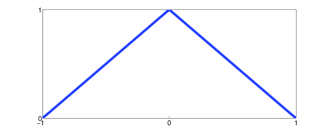
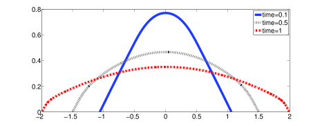
Figure 1: Left: initial datum. Right: Evolution of $u_{0}$ in case $m=1$ at different times.

Consider now $m=1$. By (1.4), $|\varphi_{t}|\leq 1$ and $\varphi_{t}(\pm\frac{1}{2}^{\mp})=\pm 1$, it follows that $(\varphi_{\eta})_{t}(\pm\frac{1}{2})\geq 0$. This implies that $\psi_{t}(\pm\frac{1}{2}^{\mp})\leq 0$ by definition of $\psi(t,\eta)$. In particular, this shows that in case $\psi(t_{0},\pm\frac{1}{2}^{\mp})=0$, this condition remains true for all time as shown in Proposition 3.2.

We define next $w(t,\eta):=\psi(t,\eta)\psi_{\eta}(t,\eta)=u_{x}(t,\varphi(t,\eta))$. The analysis above also shows that, in case $\psi(t_{0},\pm\frac{1}{2}^{\mp})=0$, then $|w(t,\pm\frac{1}{2})|\leq|w(0,\pm\frac{1}{2})|$. On the other hand, in the bulk, $w$ verifies the following equation

$$w_{t}=\frac{\psi^{5}w_{\eta\eta}}{(\psi^{2}+w^{2})^{\frac{3}{2}}}+\frac{3\psi w}{(\psi^{2}+w^{2})^{\frac{5}{2}}}(2w^{2}w_{\eta}\psi^{2}-w_{\eta}^{2}\psi^{4}-w^{4}).$$

Thus, if $w_{0}$ is initially bounded, $w$ remains bounded in $[-\frac{1}{2},\frac{1}{2}]$ as proved in Section 3. Observe that at a point $\eta_{0}$ of maximum of $w$, we have

$$w_{t}(\eta_{0})\leq-\frac{3\psi w^{5}}{(\psi^{2}+w^{2})^{\frac{5}{2}}}(\eta_{0})\leq 0,$$

implying the claim.

We show a numerical experiment with $u_{0}(x)=(1-|x|)_{+}$ as initial datum which does not satisfy the conditions of Theorem 1.1. We take $N=1000$ for the simulations. We point out that since the initial datum is $0$ at the extremes of the support, we need a lot of nodes in the discretization near them since due to the change of variables (4.3), then $\varphi_{\eta}(\pm\frac{1}{2}^{\mp})=\mp\infty$ and we want the numerical scheme to be able to capture this feature. We report in Fig. 1 the precise evolution of the support showing the smoothing effect at $x=0$, the boundedness of the derivative all over the support including the boundaries, and the expansion of the boundary at precise unit speed as expected by the theory in Theorem 1.1 and the heuristic arguments above.

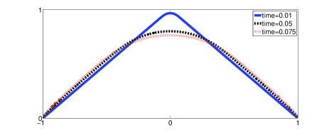
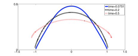
Figure 2: Evolution of $u_{0}$ in case $m=1.5$ at different times. Left: Before the discontinuity at the tip of the support appears. Right: Evolution of the discontinuity front after.

Let us now take $m>1$. In case $u(\pm A(0)^{\mp})=0$ (i.e. $\psi(0,\pm\frac{1}{2}^{\mp})=0$), then (4.8) implies that the support of the solution does not move at all whenever $u(\pm A(t))=0$. The solution will become positive at the tip of the support $u(\pm A(t))>0$ with $t>t_{0}>0$ if and only if $\psi_{t}(t_{0},\pm\frac{1}{2}^{\mp})\in(0,+\infty]$ with $u(\pm A(t_{0})^{\mp})=\psi(t_{0},\pm\frac{1}{2}^{\mp})=0$. In case $u_{x}(\pm A(t_{0}))\neq 0$, we can use (4.11) to approximate terms $(1+\psi_{\eta}^{2})^{1/2}\simeq\psi_{\eta}$ around $\pm\frac{1}{2}$ in the expression of (4.9) to get

$$\psi_{t}(t_{0},\pm\tfrac{1}{2})=\lim_{\eta\to\pm\frac{1}{2}}\psi_{t}(t_{0},\eta)=\lim_{\eta\to\pm\frac{1}{2}}(m-1)(\psi^{m}\psi_{\eta})(t_{0},\eta).$$

As a consequence, $\psi_{t}(t_{0},\pm\tfrac{1}{2}^{\mp})>0$ if and only if

$$\lim_{\eta\to\pm\frac{1}{2}}(\psi^{m+1})_{\eta}(t_{0},\eta)>0\,.$$ (4.12)

Observe that this condition in (4.12) is implied by

$$\lim_{x\to\pm A(t)}(u^{m+1}(x))_{x}(t_{0},\pm A(t))>0\,.$$

In such case, the solution becomes positive at $\pm A(t)$ and then, according to (4.8), its support starts to increase. We note that this waiting time phenomenon is similar to that of the classical porous medium equation but the condition for the support to start moving is completely different to the one obtained in [11]. Supposing a potential growth of $\psi$, i.e. $\psi(t_{0},\eta)\simeq C\left(t_{0},\frac{1}{2}-|\eta|\right)^{p}$, $p>0$, for $\eta\to\pm\frac{1}{2}^{\mp}$, then we obtain that $\psi_{t}(t_{0}\pm\frac{1}{2}^{\mp})=+\infty$ if and only if $p<\frac{1}{m+1}$.

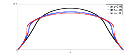
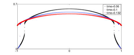
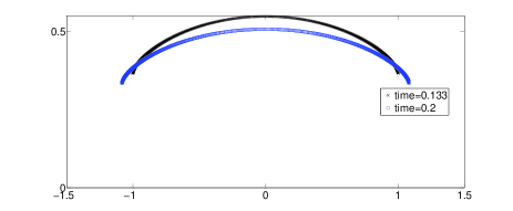
Figure 3: Evolution of $u_{0}$ in case $m=3$ at different times. Top left: Before a discontinuity on the bulk appears. Top right: After the discontinuity front forms till it reaches the tip of the support. Bottom: After the discontinuity front starts to move.

We point out that this behavior has already been numerically obtained in [10]. In Fig. 2, we show this waiting time phenomenon for $m=1.5$. One can observe that initially the support does not move since the behavior near the boundary is $\psi(0,\eta)\simeq C\left(0,\frac{1}{2}-|\eta|\right)^{\frac{1}{2}}$, then the derivative at the boundary builds up until the behavior at the boundary reaches the critical value producing the lift-off of the boundary point. More interesting is the case $m=3$ which we show in Fig. 3. There, a discontinuity in the bulk appears before the support starts to move.

4.2.2 Formation of discontinuities in the bulk

In view of the first example in the last section, one may think that discontinuities may appear only as a consequence of the waiting time phenomenon; i.e. particles tend to dissipate but their support does not move, which may create the discontinuities. In this section we heuristically study that it is possible to create discontinuities inside the bulk even if the solution are far away from zero as seen in Fig. 3.

First we treat the case $m=1$. In case of an upwards jump discontinuity or a vertical angle at a point $\eta_{0}\in]-\frac{1}{2},\frac{1}{2}[$ such that $\psi_{\eta}(\eta_{0})^{\pm}=+\infty$ , then we also have $\varphi_{t}(\eta_{0})=-1$. Since $|\varphi_{t}|\leq 1$, then $\varphi_{t}(\eta_{0})=-1$ implies that $\varphi_{t}$ is nonincreasing to the left and nondecreasing to the right of $\eta_{0}$, i.e., $((\varphi_{\eta})^{-})_{t}\leq 0$ and $((\varphi_{\eta})^{+})_{t}\geq 0$. This shows that $(\psi(\eta_{0})^{-})_{t}\geq 0$ while $(\psi(\eta_{0})^{+})_{t}\leq 0$, which implies that the size of the discontinuity reduces in for an upwards jump discontinuity or that no discontinuity is created if initially there is a vertical angle.

This last phenomenon is not true if $m>1$ in the case of a vertical angle at a point $\eta_{0}\in]-\frac{1}{2},\frac{1}{2}[$ such that $\psi_{\eta}(\eta_{0})^{\pm}=+\infty$. From the equation (4.9) for $\psi$ as in previous subsection, we deduce that $\psi_{t}(\eta_{0})=(m-1)\psi^{m}\psi_{\eta}(\eta_{0})$, and thus, a discontinuity is created. Once we have a discontinuity at $\eta_{0}$ the evolution is theoretically unknown.

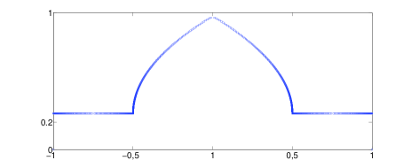
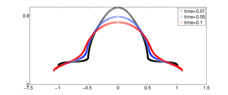
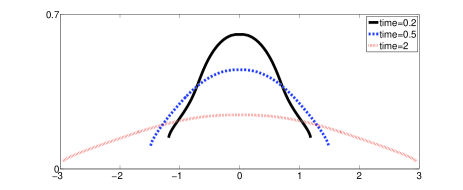
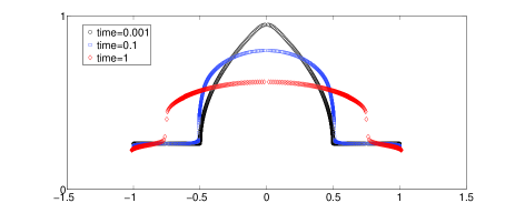
Figure 4: Evolution of solutions corresponding to $u_{0}$. Top left: Initial datum $u_{0}$. Top right: Evolution for $m=1$ at small times. Bottom left: Evolution for $m=1$ for larger times. Bottom right: Evolution for $m=4$.

In order to show this behavior we have taken two types of initial datum with $N=1000$:

$$u_{0}(x):=\frac{1}{4}\chi_{[-1,1]}+\frac{3}{2\sqrt{2}}\sqrt{\frac{1}{2}-|x|}\chi_{[-\frac{1}{2},\frac{1}{2}]}\qquad\mbox{ and }\qquad\tilde{u}_{0}(x):=\frac{1}{4}\chi_{[-1,-\frac{1}{2}]\cup[\frac{1}{2},1]}+\frac{3}{4}\chi_{]-\frac{1}{2},\frac{1}{2}[}\,.$$

We imposed a high concentration of nodes around the vertical angles or discontinuities (i.e. $x=\pm\frac{1}{2}$).

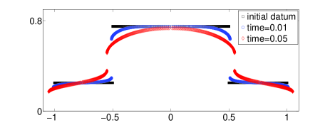
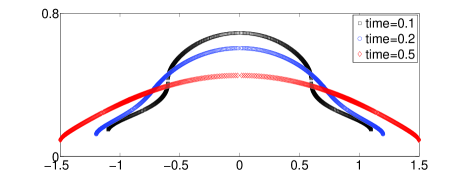
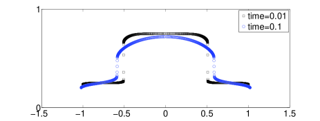
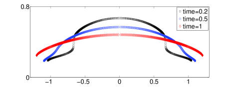
Figure 5: Evolution of solutions for $\tilde{u}_{0}$. Top: Evolution for $m=1$ at different times. Bottom: Evolution for $m=2$ at different times.

In Fig. 4 we observe the evolution of the solutions corresponding to the initial datum $u_{0}$, demonstrating the above heuristics. In Fig. 5, we see how an initially discontinuous initial datum $\tilde{u}_{0}$ is smoothed during the evolution both for $m=1$ (as heuristically deduced before) and for $m=2$. We observe that the smoothing of the discontinuity is slower with $m>1$ than that of $m=1$.

4.3 Asymptotic behavior

In this Section, guided by heuristics, we numerically observe the asymptotic behavior of solutions to (4.1) and the rate of convergence towards their asymptotic steady state, for which no result is available in the literature. Performing the classical self-similar change of variables [17] that translates porous medium equation onto nonlinear Fokker-Planck equations given by

$$v(x,t)=e^{t}u(e^{t}x,k(e^{\frac{t}{k}}-1))\,,$$ (4.13)

with $k=\frac{1}{m+1}$, then equation (4.1) transforms into

$$v_{t}={\rm div}\left(xv+\frac{v^{m}\nabla v}{\sqrt{v^{2}+e^{-2t}|\nabla v|^{2}}}\right)\,.$$ (4.14)

Therefore, formally, when $t\to\infty$ solutions of (4.14) should converge to a stationary solution of $v_{t}={\rm div}\left(xv+v^{m-1}\nabla v\right)$, i.e., to a Gaussian $V(x)$ for $m=1$ or to the corresponding Barenblatt solution $V_{m}(x)$ when $m>1$ given by

$$V(x)=\frac{1}{\sqrt{2\pi}}e^{-\frac{x^{2}}{2}}\qquad\mbox{and}\qquad V_{m}(x)=\left(C_{m}-\frac{m-1}{2}x^{2}\right)_{+}^{\frac{1}{m-1}}\,,$$

where $C_{m}$ is uniquely determined by the conservation of mass. In the original variables, then solutions should converge to the corresponding self-similar profiles obtained from $V$ and $V_{m}$ via the change of variables (4.13) except time translations. To be precise, the self-similar solutions are given by

$$U(|x|,t)=\frac{e^{-\frac{x^{2}}{4t}}}{\sqrt{4\pi t}}\,\mbox{ for }m=1\mbox{ and }\,\,U_{m}(|x|,t)=t^{\frac{-1}{m+1}}\left(\tilde{C}_{m}-\frac{m-1}{2m(m+1)}|x|^{2}t^{\frac{-2}{m+1}}\right)_{+}^{\frac{1}{m-1}}\mbox{ for }m>1,$$

where $\tilde{C}_{m}$ is determined as above.

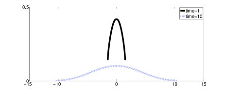
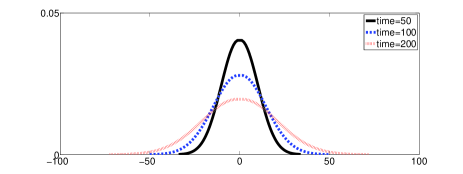
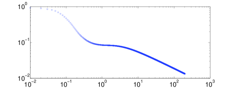
Figure 6: Top and Bottom left: Evolution of $u_{0}$ in case $m=1$ at different times with $N=100$. Bottom right: log-log plot of the estimate $\|u(t)-U(t)\|_{1}$ with $N=1000$.

In the following computations we have taken $u_{0}:=\chi_{[-\frac{1}{2},\frac{1}{2}]}$, $N=100$. We plot the evolution of the initial datum for different values of $m$ and an estimate of the difference of $u-U_{m}$ in the $L^{1}$-norm. More precisely, we took $\|u(t)-U_{m}(t)\|_{1}:=\frac{1}{N}\sum_{i=1}^{N}|u(x_{i},t)-U_{m}(x_{i},t)|$.

Some comments are in order. First of all, in Figure 6, we note that for $m=1$, while time is small, the numerical solution satisfies both the linear propagation of the support property, as well as the vertical contact angle property. However, for larger times, these two conditions are lost during the computation. This is due to the fact that we took a fixed number of nodes ($N=100$), and as time increases, this number of nodes is clearly insufficient. We have observed that by increasing the number of nodes (for instance to $N=1000$) the time in which the numerical solution is more accurate increases. We can also see in Figure 6, that, in spite of this, the numerical solution tends to a Gaussian with an algebraic rate of convergence that seems to be $\tfrac{1}{2}$ the one of the heat equation. However, it is exactly by the same reason as before that when time increases, the rate of convergence degenerates. For this reason, we have included in Figure 6 the $L^{1}$-convergence rate with $N=1000$.

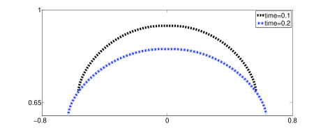
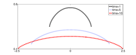
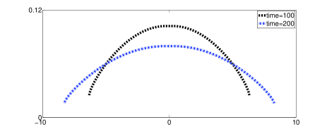
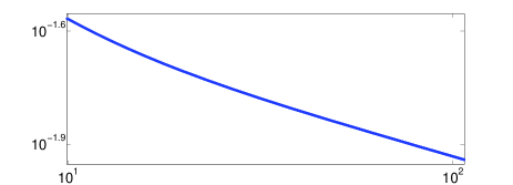
Figure 7: Top and Bottom left: Evolution of $u_{0}$ in case $m=2$ at different times. Bottom right: log-log plot of the estimate $\|u(t)-U_{2}(t)\|_{1}$.

Instead, when $m>1$, the support of the solution does not propagate so fast and we can observe in Figures 7 and 8 how the vertical contact angle property is preserved even for large times. Moreover, in Figures 7 and 8 we can see how the numerical solution tends to $U_{m}$ for $m=2$ and $m=10$. In both cases, the rate of convergence is algebraic and, numerically, it is surprisingly seen that it might correspond to $\frac{1}{3}$ in the first case and to $\frac{1}{11}$ in the second one; i.e.: the same convergence rate as for the porous medium equation, see [17, 33].

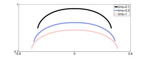
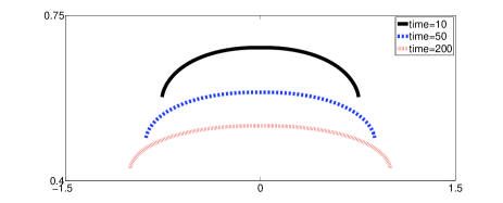
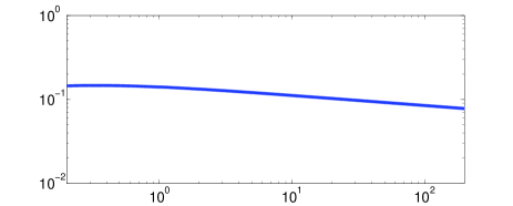
Figure 8: Top: Evolution of $u_{0}$ in case $m=10$ at different times. Bottom left: log-log plot of the estimate $\|u(t)-U_{10}(t)\|_{1}$. Bottom right: zoom of the final time interval

4.4 Convergence toward the homogeneous relativistic heat equation

We finally show numerically how solutions to (1.1), converge to solutions of the homogeneous relativistic heat equation

$$\left\{\begin{array}[]{cc}\displaystyle u_{t}=\left(u\frac{u_{x}}{|u_{x}|}\right)_{x}&{\rm in\ }I\!\!R^{N}\times[0,T]\\ u_{0}(x)=u_{0}&{\rm in\ }I\!\!R^{N}\end{array}\right.$$

when the kinematic viscosity $\nu\to+\infty$ as already proved in [7]. In Fig. 9 we estimate the evolution in time of the difference in the $L^{1}$-norm for solutions corresponding to the initial data $u_{0}=\chi_{[-\frac{1}{2},\frac{1}{2}]}$ for different values of $\nu$ with respect to the explicit solution $u_{hom}$, given by

$$u_{hom}(x,t)=\frac{1}{1+2t}\chi_{[-\frac{1}{2}-t,\frac{1}{2}+t]}$$

when $\nu\to\infty$.

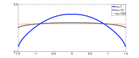
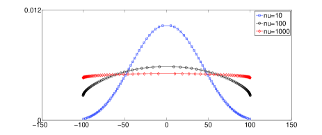
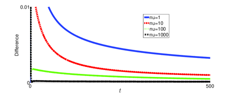
Figure 9: Top left: Numerical solution at $t=1$ for different values of $\nu$. Top Right: Numerical solution at $t=100$ for different values of $\nu$. Bottom: Evolution of the $L^{1}$-difference with respect to $u_{hom}$.

Appendix: A primer on Entropy Solutions

We collect in this Appendix some definitions that are needed to work with entropy solutions of flux limited diffusion equations.

Note that the equation (1.3) can be written as

$$u_{t}={\bf b}(u,u_{x})_{x},\qquad\hbox{in \hskip 5.69046pt $Q_{T}=(0,T)\times I\!\!R$}$$ (A.1)

where ${\bf b}(z,\xi)=\nabla_{\xi}f(z,\xi)$ and

$$f(z,\xi)=z\sqrt{z^{2}+|\xi|^{2}}.$$ (A.2)

As usual, we define

$$h(z,\xi)={\bf b}(z,\xi)\cdot\xi=\frac{z|\xi|^{2}}{\sqrt{z^{2}+|\xi|^{2}}}.$$ (A.3)

Note that $f$ is convex in $\xi$ and both $f,h$ have linear growth as $|\xi|\to\infty$.

A.1 Functions of bounded variation and some generalizations

Denote by ${\mathcal{L}}^{N}$ and ${\mathcal{H}}^{N-1}$ the $N$-dimensional Lebesgue measure and the $(N-1)$-dimensional Hausdorff measure in $I\!\!R^{N}$, respectively. Given an open set $\Omega$ in $I\!\!R^{N}$ we denote by ${\mathcal{D}}(\Omega)$ the space of infinitely differentiable functions with compact support in $\Omega$. The space of continuous functions with compact support in $I\!\!R^{N}$ will be denoted by $C_{c}(I\!\!R^{N})$.

Recall that if $\Omega$ is an open subset of $I\!\!R^{N}$, a function $u\in L^{1}(\Omega)$ whose gradient $Du$ in the sense of distributions is a vector valued Radon measure with finite total variation in $\Omega$ is called a function of bounded variation. The class of such functions will be denoted by $BV(\Omega)$. For $u\in BV(\Omega)$, the vector measure $Du$ decomposes into its absolutely continuous and singular parts $Du=D^{ac}u+D^{s}u$. Then $D^{ac}u=\nabla u\ \mathcal{L}^{N}$, where $\nabla u$ is the Radon–Nikodym derivative of the measure $Du$ with respect to the Lebesgue measure $\mathcal{L}^{N}$. We also split $D^{s}u$ in two parts: the jump part $D^{j}u$ and the Cantor part $D^{c}u$. It is well known (see for instance [1]) that

$$D^{j}u=(u^{+}-u^{-})\nu_{u}\mathcal{H}^{N-1}\mathbin{\vrule height=9.0pt,width=0.1pt\vrule height=0.1pt,width=9.0pt}J_{u},$$

where $u^{+}(x),u^{-}(x)$ denote the upper and lower approximate limits of $u$ at $x$, $J_{u}$ denotes the set of approximate jump points of $u$ (i.e. points $x\in\Omega$ for which $u^{+}(x)>u^{-}(x)$), and $\nu_{u}(x)=\frac{Du}{|Du|}(x)$, being $\frac{Du}{|Du|}$ the Radon–Nikodym derivative of $Du$ with respect to its total variation $|Du|$. For further information concerning functions of bounded variation we refer to [1].

We need to consider the following truncation functions. For $a<b$, let $T_{a,b}(r):=\max(\min(b,r),a)$, $T_{a,b}^{l}=T_{a,b}-l$. We denote

$$\mathcal{T}_{r}:=\{T_{a,b}\ :\ 0<a<b\},\ \ \$$

$$\mathcal{T}^{+}:=\{T_{a,b}^{l}\ :\ 0<a<b,\,l\in I\!\!R,\,T_{a,b}^{l}\geq 0\}.\ \ \$$

Given any function $w$ and $a,b\in I\!\!R$ we shall use the notation $\{w\geq a\}=\{x\in I\!\!R^{N}:w(x)\geq a\}$, $\{a\leq w\leq b\}=\{x\in I\!\!R^{N}:a\leq w(x)\leq b\}$, and similarly for the sets $\{w>a\}$, $\{w\leq a\}$, $\{w<a\}$, etc.

We need to consider the following function space

$$TBV_{\rm r}^{+}(I\!\!R^{N}):=\left\{w\in L^{1}(I\!\!R^{N})^{+}\ :\ \ T_{a,b}(w)-a\in BV(I\!\!R^{N}),\ \ \forall\ T_{a,b}\in\mathcal{T}_{r}\right\}.$$

Notice that $TBV_{\rm r}^{+}(I\!\!R^{N})$ is closely related to the space $GBV(I\!\!R^{N})$ of generalized functions of bounded variation introduced by E. Di Giorgi and L. Ambrosio in [1]. Using the chain rule for BV-functions (see for instance [1]), one can give a sense to $\nabla u$ for a function $u\in TBV^{+}(I\!\!R^{N})$ as the unique function $v$ which satisfies

$$\nabla T_{a,b}(u)=v\raisebox{2.0pt}{\rm{$\chi$}}_{\{a<u<b\}}\ \ \ \ \ {\mathcal{L}}^{N}-{\rm a.e.},\ \ \forall\ T_{a,b}\in\mathcal{T}_{r}.$$

We refer to [1] for details.

A.2 Functionals defined on BV

In order to define the notion of entropy solutions of (A.1) and give a characterization of them, we need a functional calculus defined on functions whose truncations are in $BV$.

Let $\Omega$ be an open subset of $I\!\!R^{N}$. Let $g:\Omega\times I\!\!R\times I\!\!R^{N}\rightarrow[0,\infty[$ be a Borel function such that

$$C(x)|\zeta|-D(x)\leq g(x,z,\zeta)\leq M^{\prime}(x)+M|\zeta|$$

for any $(x,z,\zeta)\in\Omega\times I\!\!R\times I\!\!R^{N}$, $|z|\leq R$, and any $R>0$, where $M$ is a positive constant and $C,D,M^{\prime}\geq 0$ are bounded Borel functions which may depend on $R$. Assume that $C,D,M^{\prime}\in L^{1}(\Omega)$.

Following Dal Maso [25] we consider the functional:

$${\mathcal{R}}_{g}(u) := \displaystyle\int_{\Omega}g(x,u(x),\nabla u(x))\,dx+\int_{\Omega}g^{0}\left(x,\tilde{u}(x),\frac{Du}{|Du|}(x)\right)\,d|D^{c}u|$$

$$+\displaystyle\int_{J_{u}}\left(\int_{u_{-}(x)}^{u_{+}(x)}g^{0}(x,s,\nu_{u}(x))\,ds\right)\,d\mathcal{H}^{N-1}(x),$$

for $u\in BV(\Omega)\cap L^{\infty}(\Omega)$, being $\tilde{u}$ is the approximated limit of $u$ [1]. The recession function $g^{0}$ of $g$ is defined by

$$g^{0}(x,z,\zeta)=\lim_{t\to 0^{+}}tg\left(x,z,\frac{\zeta}{t}\right).$$

It is convex and homogeneous of degree $1$ in $\zeta$.

In case that $\Omega$ is a bounded set, and under standard continuity and coercivity assumptions, Dal Maso proved in [25] that ${\mathcal{R}}_{g}(u)$ is $L^{1}$-lower semi-continuous for $u\in BV(\Omega)$. More recently, De Cicco, Fusco, and Verde [27] have obtained a very general result about the $L^{1}$-lower semi-continuity of ${\mathcal{R}}_{g}$ in $BV(I\!\!R^{N})$.

Assume that $g:I\!\!R\times I\!\!R^{N}\to[0,\infty[$ is a Borel function such that

$$C|\zeta|-D\leq g(z,\zeta)\leq M(1+|\zeta|)\qquad\forall(z,\zeta)\in I\!\!R^{N},\,|z|\leq R,$$ (A.4)

for any $R>0$ and for some constants $C,D,M\geq 0$ which may depend on $R$. Observe that both functions $f,h$ defined in (A.2), (A.3) satisfy (A.4).

Assume that

$$\raisebox{2.0pt}{\rm{$\chi$}}_{\{u\leq a\}}\left(g(u(x),0)-g(a,0)\right),\raisebox{2.0pt}{\rm{$\chi$}}_{\{u\geq b\}}\left(g(u(x),0)-g(b,0)\right)\in L^{1}(I\!\!R^{N}),$$

for any $u\in L^{1}(I\!\!R^{N})^{+}$. Let $u\in TBV_{\rm r}^{+}(I\!\!R^{N})\cap L^{\infty}(I\!\!R^{N})$ and $T=T_{a,b}-l\in{\mathcal{T}}^{+}$. For each $\phi\in C_{c}(I\!\!R^{N})$, $\phi\geq 0$, we define the Radon measure $g(u,DT(u))$ by

$$\langle g(u,DT(u)),\phi\rangle := {\mathcal{R}}_{\phi g}(T_{a,b}(u))+\displaystyle\int_{\{u\leq a\}}\phi(x)\left(g(u(x),0)-g(a,0)\right)\,dx$$ (A.5)

$$\displaystyle+\int_{\{u\geq b\}}\phi(x)\left(g(u(x),0)-g(b,0)\right)\,dx.$$

If $\phi\in C_{c}(I\!\!R^{N})$, we write $\phi=\phi^{+}-\phi^{-}$ with $\phi^{+}=\max(\phi,0)$, $\phi^{-}=-\min(\phi,0)$, and we define $\langle g(u,DT(u)),\phi\rangle:=\langle g(u,DT(u)),\phi^{+}\rangle-\langle g(u,DT(u)),\phi^{-}\rangle$.

Recall that, if $g(z,\zeta)$ is continuous in $(z,\zeta)$, convex in $\zeta$ for any $z\in I\!\!R$, and $\phi\in C^{1}(I\!\!R^{N})^{+}$ has compact support, then $\langle g(u,DT(u)),\phi\rangle$ is lower semi-continuous in $TBV^{+}(I\!\!R^{N})$ with respect to $L^{1}(I\!\!R^{N})$-convergence [27]. This property is used to prove existence of solutions of (A.1).

We can now define the required functional calculus (see [4, 5, 21]).

Let us denote by ${\mathcal{P}}$ the set of Lipschitz continuous functions $p:[0,+\infty[\rightarrow I\!\!R$ satisfying $p^{\prime}(s)=0$ for $s$ large enough. We write ${\mathcal{P}}^{+}:=\{p\in{\mathcal{P}}\ :\ p\geq 0\}$.

Let $S\in\mathcal{P}^{+}$, $T\in\mathcal{T}^{+}$. We assume that $u\in TBV_{\rm r}^{+}(I\!\!R^{N})\cap L^{\infty}(I\!\!R^{N})$ and note that

$$\raisebox{2.0pt}{\rm{$\chi$}}_{\{u\leq a\}}S(u)\left(f(u(x),0)-f(a,0)\right),\raisebox{2.0pt}{\rm{$\chi$}}_{\{u\geq b\}}S(u)\left(f(u(x),0)-f(b,0)\right)\in L^{1}(I\!\!R^{N}).$$

Since $h(z,0)=0$, the last assumption clearly holds also for $h$. We define by $f_{S}(u,DT(u))$, $h_{S}(u,DT(u))$ as the Radon measures given by (A.5) with $f_{S}(z,\zeta)=S(z)f(z,\zeta)$. and $h_{S}(z,\zeta)=S(z)h(z,\zeta)$, respectively.

A.3 The notion of of entropy solution

Let $L^{1}_{w}(0,T,BV(I\!\!R^{N}))$ be the space of weakly^∗ measurable functions $w:[0,T]\to BV(I\!\!R^{N})$ (i.e., $t\in[0,T]\to\langle w(t),\phi\rangle$ is measurable for every $\phi$ in the predual of $BV(I\!\!R^{N})$) such that $\int_{0}^{T}\|w(t)\|_{BV}\,dt<\infty$. Observe that, since $BV(I\!\!R^{N})$ has a separable predual (see [1]), it follows easily that the map $t\in[0,T]\to\|w(t)\|_{BV}$ is measurable. By $L^{1}_{loc,w}(0,T,BV(I\!\!R^{N}))$ we denote the space of weakly^∗ measurable functions $w:[0,T]\to BV(I\!\!R^{N})$ such that the map $t\in[0,T]\to\|w(t)\|_{BV}$ is in $L^{1}_{loc}(]0,T[)$.

Definition 4.1.

Assume that $u_{0}\in(L^{1}(I\!\!R^{N})\cap L^{\infty}(I\!\!R^{N}))^{+}$. A measurable function $u:]0,T[\times I\!\!R^{N}\rightarrow I\!\!R$ is an entropy solution of (A.1) in $Q_{T}=]0,T[\times I\!\!R^{N}$ if $u\in C([0,T];L^{1}(I\!\!R^{N}))$, $T_{a,b}(u(\cdot))-a\in L^{1}_{loc,w}(0,T,BV(I\!\!R^{N}))$ for all $0<a<b$, and

• $u(0)=u_{0}$, and

• the following inequality is satisfied

  $$\displaystyle\int_{0}^{T}\int_{I\!\!R^{N}}\phi h_{S}(u,DT(u))\,dt+\int_{0}^{T}\int_{I\!\!R^{N}}\phi h_{T}(u,DS(u))\,dt$$

  $$\leq\displaystyle\int_{0}^{T}\int_{I\!\!R^{N}}\Big{\{}J_{TS}(u(t))\phi^{\prime}(t)-{\bf b}(u(t),\nabla u(t))\cdot\nabla\phi\ T(u(t))S(u(t))\Big{\}}dxdt,$$

  for truncation functions $S,T\in\mathcal{T}^{+}$, and any smooth function $\phi$ of compact support, in particular those of the form $\phi(t,x)=\phi_{1}(t)\rho(x)$, $\phi_{1}\in{\mathcal{D}}(]0,T[)$, $\rho\in{\mathcal{D}}(I\!\!R^{N})$, where $J_{q}(r)$ denotes the primitive of $q$ for any function $q$; i.e. $\displaystyle J_{q}(r):=\int_{0}^{r}q(s)\,ds$

Acknowledgements. JAC acknowledges partial support by MICINN project, reference MICINN MTM2011-27739-C04-02, by GRC 2009 SGR 345 by the Generalitat de Catalunya, and by the Engineering and Physical Sciences Research Council grant number EP/K008404/1. JAC also acknowledges support from the Royal Society through a Wolfson Research Merit Award. VC acknowledges partial support by MICINN project, reference MTM2009-08171, by GRC reference 2009 SGR 773 and by ”ICREA Acadèmia” prize for excellence in research funded both by the Generalitat de Catalunya. S. Moll acknowledges partial support by MICINN project, reference MTM2012-31103.

References

- [1] L. AMBROSIO, N. FUSCO & D. PALLARA. Functions of Bounded Variation and Free Discontinuity Problems. Oxford Mathematical Monographs, 2000.
- [2] F. ANDREU, V. CASELLES & J.M. MAZÓN. Existence and uniqueness of solution for a parabolic quasilinear problem for linear growth functionals with data. Math. Ann. 322 (2002), 139-206.
- [3] F. ANDREU-VAILLO, V. CASELLES & J.M. MAZÓN. Parabolic Quasilinear Equations Minimizing Linear Growth Functionals. Progress in Mathematics 223, Birkhauser Verlag, 2004.
- [4] F. ANDREU, V. CASELLES & J.M. MAZÓN. A Strongly Degenerate Quasilinear Elliptic Equation. Nonlinear Analysis TMA. 61 (2005), 637-669.
- [5] F. ANDREU, V. CASELLES & J.M. MAZÓN. The Cauchy Problem for a Strong Degenerate Quasilinear Equation. J. Europ. Math. Soc. 7 (2005), 361-393.
- [6] F. ANDREU, V. CASELLES , J.M. MAZÓN & S. MOLL . Finite Propagation Speed for Limited Flux Diffusion Equations. Arch. Ration. Mech. Anal. 182 (2006), 269–297.
- [7] F. ANDREU, V. CASELLES , J.M. MAZÓN & S. MOLL. A Diffusion Equation in Transparent Media, Journal of Evolution Equations 7(1), (2007), 113–143.
- [8] F. ANDREU, V. CASELLES & J.M. MAZÓN. Some regularity results on the ‘relativistic’ heat equation. Journal of Differential Equations 245 (2008), 3639-3663.
- [9] F. ANDREU, V. CASELLES , J.M. MAZÓN & S. MOLL. The Dirichlet problem associated to the relativistic heat equation. Mathematisches Annalen 347 (2010), 135–199.
- [10] F. ANDREU, V. CASELLES , J.M. MAZÓN, J. SOLER & M. VERBENI. Radially Symmetric Solutions of a Tempered Diffusion Equation. A Porous Media, Flux-Limited Case, SIAM J. Math. Anal, 44(2) (2012), 1019–1049.
- [11] D. G. ARONSON, L. CAFFARELLI & S. KAMIN. How an initially stationary interface begins to move in porous medium flow, SIAM J. Math. Anal. 14 (1983), 639–658.
- [12] M. BERTSCH & R. DAL PASSO. Hyperbolic Phenomena in a Strongly Degenerate Parabolic Equation, Arch Rational Mech. Anal. 117 (1992), 349-387.
- [13] A. BLANCHET, V. CALVEZ & J.A. CARRILLO, Convergence of the mass-transport steepest descent scheme for the subcritical Patlak-Keller-Segel model, SIAM J. Numer. Anal., 46 (2008), 691–721.
- [14] Y. BRENIER. Extended Monge-Kantorovich Theory. in Optimal Transportation and Applications: Lectures given at the C.I.M.E. Summer School help in Martina Franca, L.A. Caffarelli and S. Salsa (eds.), Lecture Notes in Math. 1813, Springer-Verlag, 2003, pp. 91-122.
- [15] J. CARRILLO & P. WITTBOLD. Uniqueness of Renormalized Solutions of Degenerate Elliptic-Parabolic problems, Jour. Diff. Equat. 156 (1999), 93-121.
- [16] J. A. CARRILLO & S. MOLL. Numerical simulation of diffusive and aggregation phenomena in nonlinear continuity equations by evolving diffeomorphisms , SIAM Journal on Scientific Computing 31 (2009), 4305–4329.
- [17] J. A. CARRILLO & G. TOSCANI, Asymptotic -decay of solutions of the porous medium equation to self-similarity, Indiana Univ. Math. J. 49 (2000), 113-141.
- [18] J. A. CARRILLO & G. TOSCANI, Wasserstein metric and large–time asymptotics of non-linear diffusion equations, New Trends in Mathematical Physics, 234 244, World Sci. Publ., Hackensack, NJ, 2004.
- [19] A. CHERTOCK, A. KURGANOV & P. ROSENAU. Formation of discontinuities in flux-saturated degenerate parabolic equations, Nonlinearity 16 (2003), 1875-1898.
- [20] V. CASELLES. Convergence of the ‘relativistic’ heat equation to the heat equation as . Publ. Mat. 51 (2007), 121 142.
- [21] V. CASELLES. On the entropy conditions for some flux limited diffusion equations. Journal Differential Equations 250 (2011), 3311-3348.
- [22] V. CASELLES. Flux limited generalized porous media diffusion equations., Preprint 2012
- [23] G.Q. CHEN & H. FRID. Divergence-Measure Fields and Hyperbolic Conservation Laws, Arch. Rational Mech. Anal. 147 (1999), 89-118.
- [24] M.G. CRANDALL & T.M. LIGGETT. Generation of Semigroups of Nonlinear Transformations on General Banach Spaces, Amer. J. Math. 93 (1971), 265-298.
- [25] G. DAL MASO. Integral representation on of -limits of variational integrals, Manuscripta Math. 30 (1980), 387–416.
- [26] R. DAL PASSO. Uniqueness of the entropy solution of a strongly degenerate parabolic equation, Comm. in Partial Diff. Equat. 18 (1993), 265-279.
- [27] V. DE CICCO, N. FUSCO & A. VERDE. On -lower semicontinuity in , J. Convex Analysis 12 (2005), 173–185.
- [28] L. GOSSE & G. TOSCANI, Identification of asymptotic decay to self-similarity for one-dimensional filtration equations, SIAM J. Numer. Anal., 43 (2006), 2590–2606.
- [29] R. JORDAN, D. KINDERLEHRER, and F. OTTO, The variational formulation of the Fokker-Planck equation, SIAM J. Math. Anal., 29 (1998), 1–17.
- [30] S.N. KRUZHKOV. First order quasilinear equations in several independent variables, Math. USSR-Sb. 10 (1970), 217-243.
- [31] O.A. LADYZENSKAJA, V.A. SOLONNIKOV, and N.N. URAL’CEVA. Linear and Quasi-linear Equations of Parabolic Type. Americal Mathematical Society, Providence, Rhode Island, 1968.
- [32] G.M. LIEBERMAN. Second order parabolic differential equations, IWorld scientific, 2005.
- [33] F. OTTO, The geometry of dissipative evolution equations: the porous medium equation, Comm. Partial Differential Equations, 26 (2001), 101–174.
- [34] A. MARQUINA, Diffusion front capturing schemes for a class of Fokker-Planck equations: application to the relativistic heat equation, J. Comput. Phys., 229 (2010), 2659 -2674.
- [35] R.J. MCCANN & M. PUEL, Constructing a relativistic heat flow by transport time steps, Ann. Inst. H. Poincar Anal. Non Lin aire, 26 (2009), 2539 2580.
- [36] D. MIHALAS & B. MIHALAS. Foundations of radiation hydrodynamics, Oxford University Press, 1984.
- [37] P. ROSENAU. Tempered Diffusion: A Transport Process with Propagating Front and Inertial Delay, Phys. Review A 46 (1992), 7371-7374.
- [38] S. SERNA, A. MARQUINA, Fronts propagating with signal dependent speed in limited diffusion and related Hamilton Jacobi formulations, Applied Numerical Mathematics (2012).
- [39] C. VILLANI, Topics in optimal transportation, Graduate Studies in Mathematics Vol. 58, Amer. Math. Soc, Providence, 2003.