The extended Lawrence-Doniach model: the temperature evolution of the in-plane magnetic field anisotropy

Abstract

Using the quasi-classical formalism we provide the description of the temperature and field-direction dependence of the in-plane upper critical field in layered superconductors, taking into account the interlayer Josephson coupling and the paramagnetic spin splitting. We generalize the Lawrence-Doniach model for the case of high magnetic fields and show that the re-entrant superconductivity is naturally described by our formalism when neglecting the Pauli pair breaking effect. We demonstrate that in layered superconductors the in-plane anisotropy of the onset of superconductivity exhibits four different temperature regimes: from the Ginzburg-Landau type in the vicinity of the critical temperature $T_{c0}$ with anisotropies of coherence lengths, up to the FFLO type induced by the strong interference between the modulation vector and the orbital effect. Our results are in agreement with the experimental measurements of the field-angle dependence of the superconducting onset temperature of the organic compound (TMTSF)₂ClO₄.

I Introduction

Since the discovery of superconductivity in the first layered compound,gamb there have been found many types of superconductors consisting of alternating conducting and insulating layers. Examples include the high-$T_{c}$ cuprates,ioffe ; clark layered ruthenates,berg the iron pnictides and oxypnictides,kami ; taka01 ; pag , graphite intercalation compounds,han ; well ; emer crystalline organic metals,buzdin00 ; sing00 ; lebe00 the various types of artificial multi-layers,goz ; sma ; uno etc. Amongst them, layered organic metals are distinctive for a number of reasons. Most of them exhibit profound reduced dimensionality reflected in the very strong charge-transfer anisotropy. The interplay between electronic correlations and enhanced dimensionality effects leads to a broad range of physical properties observed in these materials. Moreover, organic metals are often available in highly clean single crystals that enables one to perform detailed band-structure measurements and to study mechanisms of superconductivity in quasi-low-dimensional electronic systems. Finally one of the most prominent property of organic layered superconductors is their robustness against high magnetic fields applied parallel to the conduction layers. Commonly known examples include Bechgaard salt superconductors (TMTSF)₂X, where anion X is PF₆, ClO₄ etc. A very large upper critical fields, which exceed the Pauli paramagnetic limit, for a magnetic field aligned parallel to their conducting layers were reported.lee04 ; oh ; yone01 In the compound (TMTSF)₂PF₆ $H_{c2}=90$ kOe,lee04 which is more than 4 times larger than $H_{P}\simeq 22$ kOe and an enhancement of almost two times over $H_{P}\simeq 27$ kOe is observed in the compound (TMTSF)₂ClO₄, $H_{c2}\simeq 50$ kOe.yone01 ; yone02

In magnetic field the superconductivity in usual type II superconductors is suppressed due to the diamagnetic currents and the Pauli pair breaking effect for singlet pairing. In layered conductors the spatial orbital motion of electrons is mostly restricted to the conducting planes, when charge carrier hopping between adjacent layers is small, and the magnetic field applied precisely parallel to the conducting planes weakly affects the orbital motion of electrons. Hence the orbital depairing is largely avoided (there is no magnetic flux inside the 2D Cooper pairs located in planes in such situation). Moreover, when the interlayer coherence length in a quasi-1D superconductor is comparable to the interlayer distance the field-induced quasi-2D (3D) $\rightarrow$ 2D dimensional crossover occurs in a high magnetic field, restoring the bare critical temperature, $T_{c0}$.gork01 ; lebe01

Various theories based on different pairing symmetries predicting the existence of high-field superconducting state have been proposed previously. Among them, a phase transition to an inhomogeneous FFLO (Fulde-Ferell-Larkin-Ovchinnikov) phase for $T<T^{\ast}\simeq 0.56T_{c0}$ or $H>H^{\ast}\simeq 1.06T_{c0}/\mu_{B}$, in which the the singlet superconducting ground state is characterized by the spatially modulated order parameter and the spin-polarization. Therefore superconducting state can be stable beyond the field set by the Pauli paramagnetic limit, $\mu_{B}H_{P}=\Delta_{0}/\sqrt{2}$, where $\Delta_{0}$ is the superconducting gap at $T=0$.lark01 ; fuld Conditions for the stabilization of the FFLO phase are rather stringent,grun namely (i) the orbital pair breaking effect should be sufficiently weaker than the Pauli paramagnetic limit, the Maki parameter $\alpha_{M}\equiv\sqrt{2}H_{c2}/H_{P}\gtrsim 1.8$; (ii) the system should be in a clean limit.asla ; taka ; adac ; akte03 ; houz ; cui A growing body of experimental evidence for the FFLO phase reported from a various measurement techniques supports this scenario.sing01 ; sing02 ; tana ; bian ; steg ; uji01 ; shin02 ; lort ; agos01 ; brow01 ; bergk ; agos02 ; agos03 ; uji02 An alternative to the FFLO phase is a triplet pairing state, when the Pauli spin-splitting destructive mechanism is absent. Within this pairing symmetry, as was shown by Lebed,lebe01 ; lebe06 the superconducting state is always stable at low temperatures and exhibits a strong re-entrant behavior in high magnetic field. So far the re-entrant superconducting phase has not been experimentally identified, at least it is difficult to make more than a tentative judgement.lee01 ; lee06 Nevertheless it can reveal itself in a number of nontrivial effects in singlet-paired organic materials in high magnetic fields.lebe03 ; lebe04 It was shown that it can appear in a hidden form and be responsible for an increase of the superconducting transition temperature in a magnetic field if the orbital effects of an electron motion are stronger than the Pauli spin-splitting effects (Paramagnetic intrinsic Meissner effect).lebe03

Hitherto there is no experiment which unequivocally answer on the lingering question concerning the superconducting pairing symmetry in (TMTSF)₂X compounds. Previously it was reported that the Knight shift in (TMTSF)₂PF₆ conductor does not change at transition temperature supporting the triplet scenario of pairing.lee04 However, later experiment with (TMTSF)₂ClO₄ conductor at low-field regime have revealed a clear change of the Knight shift at the superconducting transition making possible consideration of the singlet scenario of pairing in such structures.shin02 In the high-field regime the Knight shift is quite weak. On the other hand, as shown in Ref. shim06 a small fraction of the triplet pairing in the singlet paired superconductor strongly enhances the upper critical field and the triplet component of the order parameter is always generated in singlet superconductors due to the Pauli paramagnetic spin-splitting effects.lebe07 ; kaba

In this paper we extend results presented in our previous Letter,vrnkch01 and investigate the in-plane magnetic field-angle dependence of the onset of superconductivity in layered conductors in the conventional and the FFLO modulated phases. For this purpose we provide the quasiclassical description of the anisotropy of the in-plane critical field in layered superconductors and generalize the Lowerence-Doniach model for the case of high magnetic fields.

The layout of our paper is as follows. In Sec.II, we outline our model based on the quasi-classical formalism for layered superconducting samples. In Sec. III we derive the generalized Lowerence-Doniach equation. In sec. IV we extend this model to the extremely high magnetic fields. In Sec. V we focus on the in-plane anisotropy of the upper critical field for layered superconductors when only orbital motion is included in the model, and then we investigate the in-plane anisotropy of $H_{c2}$ when both orbital and paramagnetic depairing are accounted for. Finally, a short summary is given, where we emphasize the significance of the obtained results for the interpretation of experiments with layered superconductors.

II General settings

We consider a system consisting of layers with good conductivity in xy-plane stacked along the z-axis [see Fig. 1]. The single-electron spectrum is taken as follows

$$E_{\mathbf{p}}=\frac{p_{x}^{2}}{2m_{x}}+\frac{p_{y}^{2}}{2m_{y}}+\varepsilon\left(p_{z}\right),$$ (1)

where $\varepsilon\left(p_{z}\right)=2t\cos\left(p_{z}d\right)$ with $d$ - the interlayer distance. We assume that the coupling between layers is small [see Fig. 2], i.e. $t\ll T_{c0}$, but sufficiently large to make the mean field treatment justified, $T_{c0}^{2}/E_{F}$ $\ll t$.tsu Here $T_{c0}$ is the critical temperature of the system at $H=0$. In purely 2D samples, phase fluctuations destroy the long-range order, however as shown in Ref. kats01 , even a very small value of hopping leads to restoration of superconducting order.

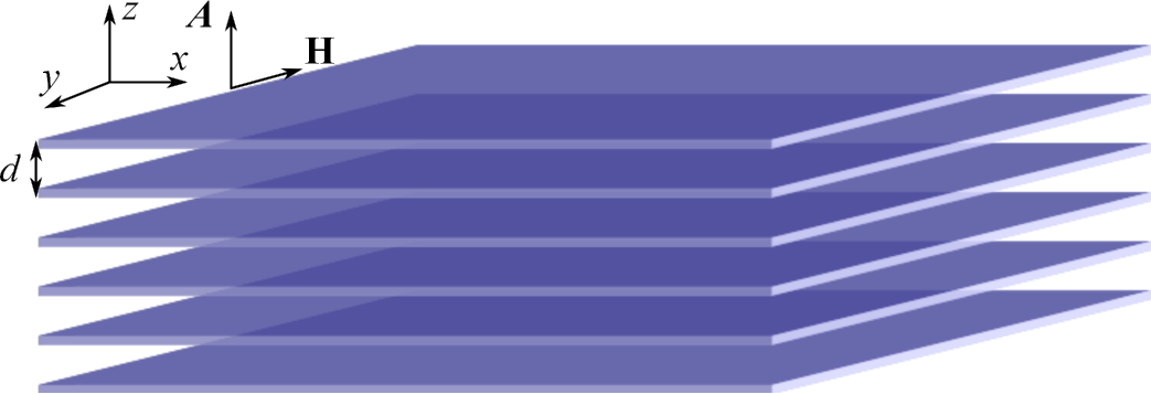
Figure 1: Scheme of the quasi-2D layered metal.

We choose the magnetic field to be parallel to the conducting planes and with a gauge for which the vector potential $\mathbf{A}=\mathbf{H}\times\mathbf{r}$ [$\mathbf{r}=(x,y,0)$ is a coordinate in xy-plane], i.e. $A_{z}=-xH\sin\alpha+yH\cos\alpha$, where $\alpha$ is the angle between the applied field, with amplitude $H$, and x-axis. Assuming that the vector potential varies slowly at the interlayer distances (this assumption means that we neglect the diamagnetic screening currents and take the magnetic field as uniform and given by the external field, $H$), and taking into account that the system is near the second-order phase transition, we can employ the linearized Eilenberger equation for a layered superconductor in the presence of the parallel magnetic field (in the momentum representation with respect to the coordinate z)kop :

$$\left(\Omega_{n}+\widehat{\Pi}\right)f_{\omega}\left(\mathbf{n},\mathbf{r},p_{z},k_{z}\right)=\left\{\Delta(\mathbf{r},k_{z})\frac{{}}{{}}\right.\\ +\left.\frac{\left\langle f_{\omega}\left(\mathbf{n},\mathbf{r},p_{z},k_{z}\right)\right\rangle}{2\tau}\right\}\mathrm{sign}(\omega_{n}).$$ (2)

Here

$$\widehat{\Pi}\equiv\frac{\hbar}{2}\mathbf{v}_{F}.\mathbf{\nabla}+2it\sin(p_{z}d)\sin(\mathbf{Q.r-}\frac{k_{z}}{2}d),$$ (3)

where $\mathbf{Q}=(\pi dH/\phi_{0})[-\sin\alpha,(m_{x}/m_{y})^{1/2}\cos\alpha,0]$ with $\phi_{0}=\pi\hbar c/e$, $h=\mu_{B}H$ is the Zeeman energy, $\mathbf{v}_{F}=v_{F}\mathbf{n}$ is the in-plane Fermi velocity, $\tau$ is the impurity scattering time, and $\Omega_{n}\equiv\omega_{n}-ih+\mathrm{sign}(\omega_{n})/2\tau$. The order parameter is defined self-consistently as

$$\frac{1}{\lambda}\Delta\left(\mathbf{r},k_{z}\right)=2\pi T\Re\sum\limits_{\omega>0}\left\langle f_{\omega}\left(\mathbf{n},\mathbf{r},p_{z},k_{z}\right)\right\rangle,$$ (4)

where $\lambda$ is the pairing constant and the brackets denote averaging over $p_{z}$ and $\mathbf{n}$,

$$\left\langle...\right\rangle\equiv\int\limits_{-\frac{\pi}{d}}^{\frac{\pi}{d}}\frac{d~{}dp_{z}}{2\pi}\int\limits_{0}^{2\pi}\frac{d\alpha}{2\pi}\left(...\right).$$ (5)

We assume that the temperature unit is so chosen that the Boltzmann constant $k_{B}=1$.

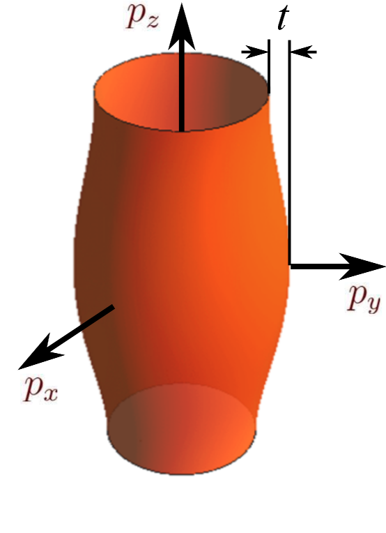
Figure 2: The Fermi surface of the layered metal in the form of a corrugated cylinder.

Here we considered a layered superconductor in the clean limit, meaning that the in-plane mean free path is much larger than the corresponding intra-plane coherence length, $\xi_{0}^{||}=\hbar v_{F}/(2\pi T_{c0})$. Therefore the linearized Eilenberger equation for the anomalous Green function $f_{\omega}(\mathbf{n},\mathbf{r},p_{z},k_{z})$ describing layered superconducting systems acquires the form

$$\left[\Omega_{n}+\widehat{\Pi}\right]f_{\omega}(\mathbf{n},\mathbf{r},p_{z},k_{z})=\Delta(\mathbf{r},k_{z})$$ (6)

with $\Omega_{n}\equiv\omega_{n}-ih~{}\mathrm{sign}(\omega_{n})$ from now on.

III A layered superconductor in a parallel magnetic field

The upper critical field corresponds to the highest value of $H$, for which the solution of Eqs. (4) and (6) exists. To start with, we consider Eq. (6) and write it in the form

$$f_{\omega}(\mathbf{n},\mathbf{r},p_{z},k_{z})=\frac{\Delta(\mathbf{r},k_{z})}{\Omega_{n}}-\frac{1}{\Omega_{n}}\widehat{\Pi}f_{\omega}(\mathbf{n},\mathbf{r},p_{z},k_{z})$$ (7)

convenient for the subsequent derivation of iterative procedure. Using this equation we construct the following iterative scheme

$$f_{\omega}^{\left(k+1\right)}\left(\mathbf{n},\mathbf{r},p_{z},k_{z}\right)=\frac{\Delta(\mathbf{r},k_{z})}{\Omega_{n}}-\frac{1}{\Omega_{n}}\widehat{\Pi}f_{\omega}^{\left(k\right)}(\mathbf{n},\mathbf{r},p_{z},k_{z}).$$ (8)

To obtain the convergent iterative scheme we need to require that $\Delta(\mathbf{r})\gg\hbar\mathbf{v}_{F}.\bm{\nabla}\Delta(\mathbf{r})/2\pi T_{c0}$, that implies that characteristic scale of the order parameter variations should be much larger than $\xi_{0}^{||}=\hbar v_{F}/2\pi T_{c0}$. After the completion of the k-th iteration we obtain

$$f_{\omega}^{\left(k+1\right)}\left(\mathbf{n},\mathbf{r},p_{z},k_{z}\right)=\sum\limits_{l=0}^{k}\frac{\left(-1\right)^{l}}{\Omega_{n}^{l+1}}\widehat{\Pi}^{l}\Delta(\mathbf{r},k_{z}).$$ (9)

Taking into account the averaging procedure over momentum $p_{z}$, and hence omitting the terms with even powers of $\sin\left(p_{z}d\right),$ then retaining terms up to the second order in $\hbar\mathbf{v}_{F}.\bm{\nabla}\Delta(\mathbf{r})/2\pi T_{c0}$, and making use of the self-consistency relation Eq. (4), we obtain the extended Lowerence-Doniach equation (MLD equation) in the isotropic case

$$\Delta\left(\mathbf{r},k_{z}\right)\ln\frac{T_{c}}{T_{c0}}=\Delta\left(\mathbf{r},k_{z}\right)\\ \times\pi T_{c}\sum\limits_{n}\left[\frac{1}{\omega_{n}}-\frac{1}{\Omega_{n}}\right]+\widehat{\Pi}_{\mathrm{MLD}}^{h\neq 0}\Delta\left(\mathbf{r},k_{z}\right)$$ (10)

where $T_{c0}$ is the critical temperature in the absence of coupling between adjacent layers, $t$, and of the magnetic field, and

$$\widehat{\Pi}_{\mathrm{MLD}}^{h\neq 0}\equiv\pi T_{c}\sum\limits_{n}\frac{\hbar^{2}v_{F}^{2}}{8\Omega_{n}^{3}}\nabla^{2}-\frac{t^{2}}{\Omega_{n}^{3}}\left[1-\cos\left(2\mathbf{Q.r-}k_{z}d\right)\right]\\ +\frac{\hbar^{2}\left(v_{F}Q\right)^{2}}{8}\frac{t^{2}}{\Omega_{n}^{5}}\left[1-7\cos\left(2\mathbf{Q.r-}k_{z}d\right)\right]$$ (11)

The anisotropic case one can obtain simply by the following substitutions $\hbar^{2}v_{F}^{2}\nabla^{2}\Delta\left(\mathbf{r}\right)\rightarrow 2\varepsilon\left(\mathbf{\nabla}\right)\Delta\left(\mathbf{r}\right)\equiv 2\hbar^{2}\left\{\left\langle v_{Fx}^{2}\right\rangle\partial_{x}^{2}+\left\langle v_{Fy}^{2}\right\rangle\partial_{y}^{2}\right\}\Delta\left(\mathbf{r}\right)$ and $\hbar^{2}\left(v_{F}Q\right)^{2}\rightarrow 2\varepsilon\left(\mathbf{Q}\right)$, where

$$\varepsilon\left(\mathbf{Q}\right)\equiv\hbar^{2}\left\{\left\langle v_{Fx}^{2}\right\rangle Q_{x}^{2}+\left\langle v_{Fy}^{2}\right\rangle Q_{y}^{2}\right\}.$$ (12)

Introducing the temperature $T_{cP}$, as the superconducting onset temperature in the pure Pauli limit determined by the expression

$$\ln\frac{T_{c0}}{T_{cP}}=\pi T_{cP}\sum\limits_{n}\left[\frac{1}{\omega_{n}}-\frac{1}{\Omega_{n}}\right],$$ (13)

and the use of the identities $2\pi T\sum\nolimits_{n=0}^{\infty}\Omega_{n}^{-3}=-\Phi^{\left(2\right)}\left(h\right)/8\pi^{2}T^{2}$ and $2\pi T\sum\nolimits_{n=0}^{\infty}\Omega_{n}^{-5}=-\Phi^{\left(4\right)}\left(h\right)/384\pi^{2}T^{2}$ gives rise to (for details see Appendix A)

$$\Delta\left(\mathbf{r},k_{z}\right)P=-\frac{\Phi^{\left(2\right)}\left(h\right)}{8\pi^{2}T_{cP}^{2}}\\ \times\left\{\frac{\varepsilon\left(\mathbf{\nabla}\right)}{4}-t^{2}\left[1-\cos\left(2\mathbf{Q.r-}k_{z}d\right)\right]\right\}\Delta\left(\mathbf{r},k_{z}\right)\\ -\frac{\Phi^{\left(4\right)}\left(h\right)t^{2}}{384\pi^{4}T_{cP}^{4}}\frac{\varepsilon\left(\mathbf{Q}\right)}{4}\left[1-7\cos\left(2\mathbf{Q.r-}k_{z}d\right)\right]\Delta\left(\mathbf{r},k_{z}\right),$$ (14)

where $P=\left(T_{c}-T_{cP}\right)/AT_{c}$, $\Phi^{\left(k\right)}\left(h\right)\equiv\left[\psi^{\left(k\right)}\left(1/2+ih\right)+\psi^{\left(k\right)}\left(1/2-ih\right)\right]/2$ with $\psi^{\left(k\right)}\left(z\right)=d^{k}\psi\left(z\right)/dz^{k}$ and $\psi\left(z\right)$ is the digamma function. If we can neglect the Zeeman effect, $h=0$, than $\Omega_{n}\rightarrow\omega_{n}$, and making use of the identities $2\pi T\sum\nolimits_{n=0}^{\infty}\omega_{n}^{-3}=7\zeta\left(3\right)/4\pi^{2}T^{2}$ and $2\pi T\sum\nolimits_{n=0}^{\infty}\omega_{n}^{-5}=31\zeta\left(5\right)/16\pi^{2}T^{2}$ reduces Eq. (14) to

$$\Delta\left(\mathbf{r},k_{z}\right)\ln\frac{T_{c}}{T_{c0}}=\frac{7\zeta\left(3\right)}{4\pi^{2}T_{c0}^{2}}\\ \times\left\{\frac{\varepsilon\left(\mathbf{\nabla}\right)}{4}-t^{2}\left[1-\cos\left(2\mathbf{Q.r-}k_{z}d\right)\right]\right\}\Delta\left(\mathbf{r},k_{z}\right)\\ +\frac{31\zeta\left(5\right)t^{2}}{16\pi^{4}T_{c0}^{4}}\frac{\varepsilon\left(\mathbf{Q}\right)}{4}\left[1-7\cos\left(2\mathbf{Q.r-}k_{z}d\right)\right]\Delta\left(\mathbf{r},k_{z}\right),$$ (15)

where $T_{c0}$ is the superconducting critical temperature in the absence of coupling between adjacent layers, $t$, and in the absence of the magnetic field, described by the vector $Q$. As it is seen the MLD equation contains the term, proportional to $\left(v_{F}Q\right)^{2}t^{2}$, which is absent in the standard Lowerence-Doniach equation. As it will be seen later this term represents unusual orbital contribution responsible for the re-entrant superconducting phase at high magnetic fields.lebe03 Let us consider several limiting cases.

III.1 Regime $H\ll\frac{t}{\pi\hbar dv_{F}}\phi_{0}$

First, let us consider the case of a small magnetic field. When $\hbar v_{F}Q$ $\ll T_{c0}$, we can retain only terms up to the second order in $\left(\hbar v_{F}Q\right)/T_{c0}$ or/and $t/T_{c0}$. Then after neglecting the last term in the MLD, because it is much smaller than other terms, Eq. (10) reduces to the standard Lowerence-Doniach equation

$$\Delta\left(\mathbf{r},k_{z}\right)P=\pi T_{c}\sum\limits_{n}\frac{\varepsilon\left(\mathbf{\nabla}\right)}{4\Omega_{n}^{3}}\Delta\left(\mathbf{r},k_{z}\right)\\ -\frac{t^{2}}{\Omega_{n}^{3}}2\sin^{2}\left(\mathbf{Q.r}-\frac{k_{z}}{2}d\right)\Delta\left(\mathbf{r},k_{z}\right).$$ (16)

In the continuous limit, $d\rightarrow 0$, $d\ll\xi_{0}^{\perp}\left(T\right)$ with $\xi_{0}^{\perp}$ - the inter-plane coherence length, Eq. (16) transforms into the Ginzburg-Landau equation for an anisotropic superconductor. If the order parameter is homogeneous along the z-axis we can set $k_{z}=0$. If $Qr\mathbf{\sim}Ql\ll 1$, or $H\ll\frac{t}{\pi\hbar dv_{F}}\phi_{0}$, where $l=\sqrt{\hbar/m\widetilde{\omega}_{H}}$ is the characteristic magnetic length with the characteristic magnetic frequency $\widetilde{\omega}_{H}$ defined as $\widetilde{\omega}_{H}=\sqrt{\frac{2\gamma_{z}}{m_{x}}T_{c0}}\frac{2\pi}{\phi_{0}}H$, Eq. (16) can be further simplified

$$P\Delta\left(\mathbf{r}\right)-\left[\gamma_{x}\partial_{x}^{2}+\gamma_{y}\partial_{y}^{2}-\gamma_{z}\left(\frac{2\mathbf{Qr}}{d}\right)^{2}\right]\Delta\left(\mathbf{r}\right)=0,$$ (17)

where $\alpha=\left(T_{c}-T_{c0}\right)/T_{c0}$, $\gamma_{x,y}=-\hbar^{2}\Phi^{\left(2\right)}\left(h\right)\left\langle v_{Fx,y}^{2}\right\rangle/32\pi^{2}T_{cP}^{2}$, $\gamma_{z}=d^{2}t^{2}\Phi^{\left(2\right)}\left(h\right)/16\pi^{2}T_{cP}^{2}$. If $h=0$ we may write $\gamma_{x,y}=\beta\hbar^{2}\left\langle v_{Fx,y}^{2}\right\rangle/2T_{c0}^{2}=\beta\hbar^{2}v_{F}^{2}/4T_{c0}^{2}$, $\gamma_{z}=\beta d^{2}t^{2}/T_{c0}^{2}$, where $\beta=7\zeta\left(3\right)/8\pi^{2}$. The cyclotron frequency is $\widetilde{\omega}_{H}=\sqrt{\frac{\gamma_{z}}{\gamma_{x}}}\frac{\hbar}{m_{x}}\frac{2\pi}{\phi_{0}}H$, or using the relation $\gamma_{x}/\gamma_{z}=\left\langle v_{Fx,y}^{2}\right\rangle/2d^{2}t^{2}=v_{F}^{2}/4d^{2}t^{2}$, is $\widetilde{\omega}_{H}=\frac{2dt}{m_{x}v_{F}}\frac{2\pi}{\phi_{0}}H$. After performing scaling of the variable $y^{\prime}=\sqrt{m_{y}/m_{x}}y$, the anisotropic model with effective masses can be reduced to the isotropic one in the renormalized magnetic field $H\rightarrow H\sqrt{\sin^{2}\left(\vartheta\right)+\frac{m_{x}}{m_{y}}\cos^{2}\left(\vartheta\right)}$,brison where $\hbar^{2}/2m_{x,y}=\gamma_{x,y}T_{c0}$. Finally, the angle-resolved highest magnetic field, at which superconductivity can nucleate in a sample is given by

$$\left.H_{c2}\left(\vartheta,T\right)\right|_{\varkappa_{I}}=\frac{\left.H_{c2}\left(\frac{\pi}{2}\right)\right|_{\varkappa_{I}}}{\sqrt{\sin^{2}\left(\vartheta\right)+\frac{m_{x}}{m_{y}}\cos^{2}\left(\vartheta\right)}}.$$ (18)

Here for the negligible Zeeman effect, which breaks apart the paired electrons if they are in a spin-singlet state, $h=0$,

$$\left.H_{c2}^{h=0}\left(\frac{\pi}{2}\right)\right|_{\varkappa_{I}}=\frac{m_{x}}{\hbar^{2}}\frac{\hbar v_{F}}{d}\frac{T_{c0}}{t}\frac{\phi_{0}}{2\pi}\left(1-\frac{T_{c}}{T_{c0}}\right),$$ (19)

while for $h\neq 0$

$$\left.H_{c2}^{h\neq 0}\left(\frac{\pi}{2}\right)\right|_{\varkappa_{I}}=\frac{8\pi T_{c0}}{A\hbar dt}\sqrt{\frac{m_{x}T_{c0}}{2\Phi^{\left(2\right)}\left(h\right)}}\frac{\phi_{0}}{2\pi}\left(1-\frac{T_{c}}{T_{cP}}\right),$$ (20)

where $\varkappa_{I}:H\ll\frac{t}{\pi\hbar dv_{F}}\phi_{0}$.

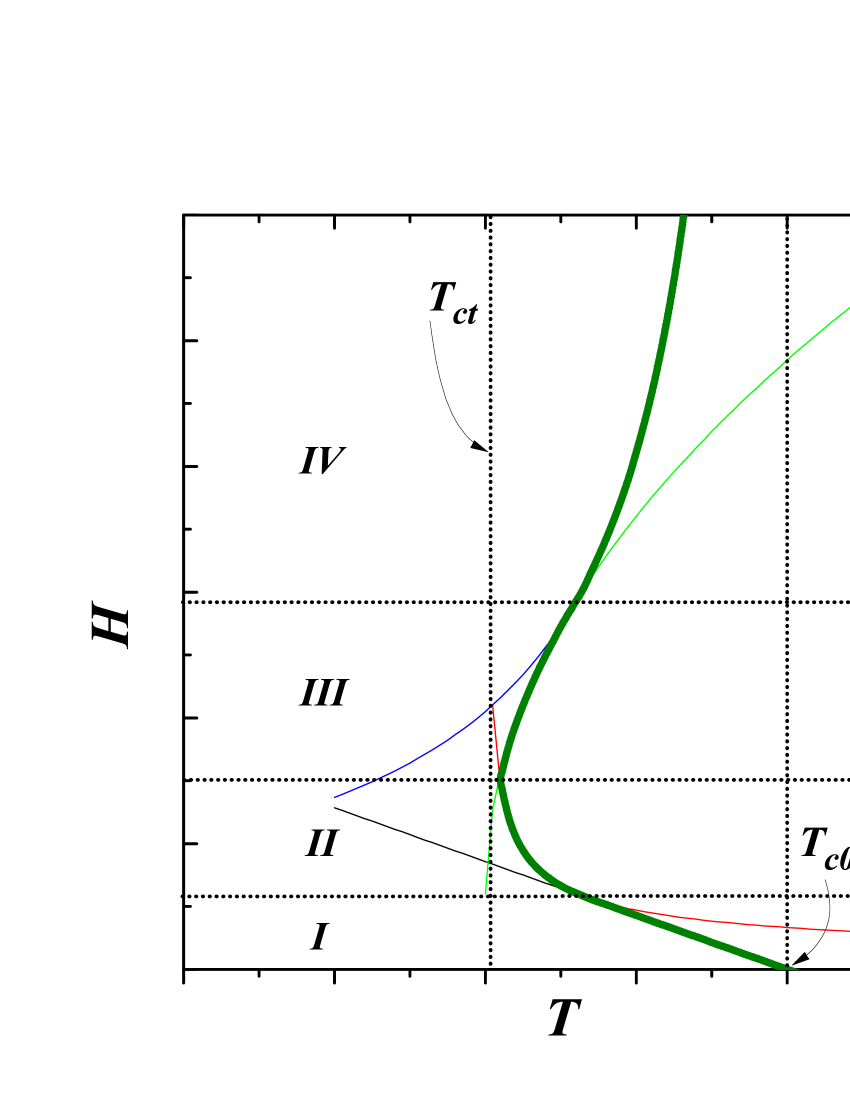
Figure 3: Scheme of the $H-T$ phase diagram for layered superconductors, when external magnetic field, $H$, is applied parallel to the layers, $t\ll T_{c0}$, and the paramagnetic effects are vanished.

III.2 The crossover regime: $\frac{\phi_{0}}{\pi\hbar dv_{F}}t\ll H\ll\frac{\phi_{0}}{\pi\hbar dv_{F}}T_{c0}$

To study the anisotropy of the upper critical field, when its amplitude is in the range, $t\ll\hbar v_{F}Q\ll T_{c0}$, or $\frac{\phi_{0}}{\pi\hbar dv_{F}}t\ll H\ll\frac{\phi_{0}}{\pi\hbar dv_{F}}T_{c0}$, we employ the extended Lowerence-Doniach equation Eq. (10) and choose the solution in the form

$$\Delta\left(\mathbf{r}\right)=\Delta_{0}+\Delta_{2}\cos\left(2\mathbf{Q.r}\right).$$ (21)

By substitution it in Eq. (10), we obtain the following system of coupled equations

$$\Delta_{0}P=\pi T_{cP}\sum\limits_{n}\left[-\frac{1}{\Omega_{n}^{3}}+\frac{\varepsilon\left(\mathbf{Q}\right)}{4\Omega_{n}^{5}}\right]t^{2}\Delta_{0}\\ +\pi T_{cP}\sum\limits_{n}\left[\frac{1}{2\Omega_{n}^{3}}-7\frac{\varepsilon\left(\mathbf{Q}\right)}{8\Omega_{n}^{5}}\right]t^{2}\Delta_{2},$$ (22)

and

$$\Delta_{2}P=-\pi T_{cP}\sum\limits_{n}\left\{\frac{\varepsilon\left(\mathbf{Q}\right)}{\Omega_{n}^{3}}\Delta_{2}\right.\\ +\left.\left(\Delta_{0}-\frac{\Delta_{2}}{2}\right)\frac{t^{2}}{\Omega_{n}^{3}}-\left(7\Delta_{0}+\frac{5\Delta_{2}}{2}\right)\frac{\varepsilon\left(\mathbf{Q}\right)t^{2}}{8\Omega_{n}^{5}}\right\}.$$ (23)

In the situation $\left|P\right|\ll\left|\Phi^{\left(2\right)}\left(h\right)\right|\varepsilon\left(\mathbf{Q}\right)/8\pi^{2}T_{cP}^{2}$, when taking into account that $\Delta_{0}\gg\Delta_{2}$, from Eq. (23) we can obtain $\Delta_{2}=t^{2}\Delta_{0}/\varepsilon\left(\mathbf{Q}\right).$ Substituting it into Eq. (22) and retaining only terms up to the second order in ($t/T_{c0}$) leads to

$$P=\pi T_{cP}\sum\limits_{n}\left[-\frac{1}{\Omega_{n}^{3}}+\frac{\varepsilon\left(\mathbf{Q}\right)}{4\Omega_{n}^{5}}+\frac{1}{2\Omega_{n}^{3}}\frac{t^{2}}{\varepsilon\left(\mathbf{Q}\right)}\right]t^{2}$$ (24)

or

$$P=\frac{\Phi^{\left(2\right)}\left(h\right)}{8\pi^{2}T_{cP}^{2}}t^{2}-\varepsilon\left(\mathbf{Q}\right)t^{2}\frac{\Phi^{\left(4\right)}\left(h\right)}{1536\pi^{2}T_{cP}^{2}}-\frac{t^{4}}{\varepsilon\left(\mathbf{Q}\right)}\frac{\Phi^{\left(2\right)}\left(h\right)}{16\pi^{2}T_{cP}^{2}}$$ (25)

If the Zeeman effect of the applied field is absent, $h=0$, we have to make the following substitution, $\Omega_{n}\rightarrow\omega_{n}$ and $T_{cP}\rightarrow T_{c0}$. After introducing the temperature, $T_{ct}$, accounting for the coupling between adjacent layers via expression $\ln\left(T_{c0}/T_{ct}\right)=t^{2}\pi T_{ct}\sum\nolimits_{n}\omega_{n}^{-3}$, Eq. (24) acquires the form

$$\ln\frac{T_{c}}{T_{ct}}=t^{2}\pi T_{c0}\sum\limits_{n}\frac{\varepsilon\left(\mathbf{Q}\right)}{4\omega_{n}^{5}}+\frac{t^{4}}{\varepsilon\left(\mathbf{Q}\right)}\pi T_{c0}\sum\limits_{n}\frac{1}{2\omega_{n}^{3}},$$ (26)

where

$$\varepsilon\left(\mathbf{Q}\right)\equiv\frac{\hbar^{2}v_{F}^{2}}{2}\frac{\pi^{2}d^{2}H^{2}}{\phi_{0}^{2}}\left[\sin^{2}\left(\vartheta\right)+\frac{m_{x}}{m_{y}}\cos^{2}\left(\vartheta\right)\right],$$ (27)

or using the definition $\left\langle v_{Fx,y}^{2}\right\rangle=\frac{T_{c0}}{\beta m_{x,y}}$,

$$\varepsilon\left(\mathbf{Q}\right)\equiv\frac{\hbar^{2}}{m_{x}}\frac{T_{c0}}{\beta}\frac{\pi^{2}d^{2}H^{2}}{\phi_{0}^{2}}\left[\sin^{2}\left(\vartheta\right)+\frac{m_{x}}{m_{y}}\cos^{2}\left(\vartheta\right)\right].$$ (28)

Eq. (26) is the transcendental equation to determine $H_{c2}\left(\vartheta,T\right)$ for a layered system with interlayer coupling $t$. Let us consider two limiting situations.

III.2.1 Lowerence-Doniach regime $t\phi_{0}/\pi\hbar dv_{F}\ll H\ll\sqrt{tT_{c0}}\phi_{0}/\pi\hbar dv_{F}$

If the amplitude of the external magnetic field satisfies the condition $t\ll\hbar v_{F}Q\ll\sqrt{tT_{c0}}$, or $t\phi_{0}/\pi\hbar dv_{F}\ll H\ll\sqrt{tT_{c0}}\phi_{0}/\pi\hbar dv_{F}$, we can neglect the first term in Eq. (26) and obtain Eq. (18), as the expression for the upper critical field with

$$\left.H_{c2}^{h=0}\left(\frac{\pi}{2}\right)\right|_{\varkappa_{II}}=\frac{7\zeta\left(3\right)t^{2}}{8\pi^{3}\hbar dT_{c0}}\sqrt{\frac{2m_{x}}{T_{c}-T_{ct}}}\phi_{0},$$ (29)

where $\varkappa_{II}:t\phi_{0}/\pi\hbar dv_{F}\ll H\ll\sqrt{tT_{c0}}\phi_{0}/\pi\hbar dv_{F}$, when the Zeeman effect is negligible.

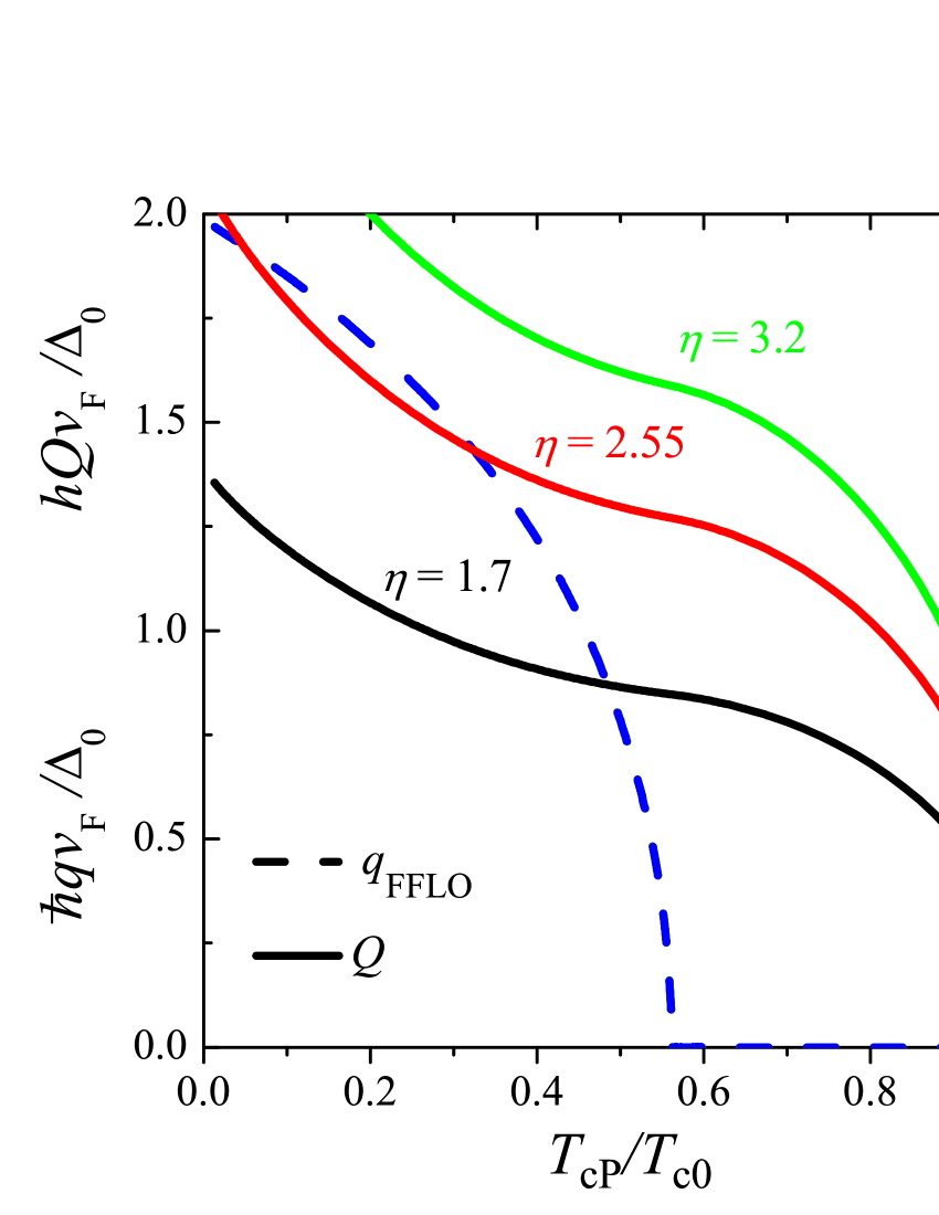
Figure 4: $\hbar qv_{F}/k_{B}T_{c0}$ and $\hbar Qv_{F}/k_{B}T_{c0}$ versus $T_{cP}/T_{c0}$ for several values of $\eta$.

III.2.2 Regime $\frac{\phi_{0}}{\pi\hbar dv_{F}}\sqrt{tT_{c0}}\ll H\ll\frac{\phi_{0}}{\pi\hbar dv_{F}}T_{c0}$

If the field is such that $\sqrt{tT_{c0}}\ll\hbar v_{F}Q\ll T_{c0}$, or $\frac{\phi_{0}}{\pi\hbar dv_{F}}\sqrt{tT_{c0}}\ll H\ll\frac{\phi_{0}}{\pi\hbar dv_{F}}T_{c0}$ the expression for the upper critical field, $H_{c2}\left(\vartheta,T\right)$, can be obtained from Eq. (26) by neglecting the second term. Then again we obtain Eq. (18), as the expression for the upper critical field with

$$\left.H_{c2}^{h=0}\left(\frac{\pi}{2}\right)\right|_{\varkappa_{III}}=\sqrt{\frac{28}{31}\frac{\zeta\left(3\right)}{\zeta\left(5\right)}}\frac{T_{c0}}{dt}\sqrt{\frac{2m_{x}\left(T_{c}-T_{ct}\right)}{\hbar^{2}}}\phi_{0}.$$ (30)

This regime describes the beginning of the reentrant superconductivity regime.lebe01 ; lebe06

IV General case for $H\gg\frac{t}{\pi\hbar dv_{F}}\phi_{0}$

To study the anisotropy of the upper critical field, when its amplitude satisfies $H\gg\frac{t}{\pi\hbar dv_{F}}\phi_{0}$ we need to reconsider the solution of the Eilenberger equation, Eq. (6). Since the magnetic field induced potential has the form $V\left(\mathbf{r}\right)=t\sin\left(p_{z}d\right)\left[e^{i\mathbf{Q.r}}-e^{-i\mathbf{Q.r}}\right]$ $=2it\sin\left(p_{z}d\right)\sin\left(\mathbf{Q.r}\right)$, i.e. it is periodic in real space, the solution of Eq. (6) can be written without any loss of generality asvrnkch01

$$f_{\omega}\left(\mathbf{n}_{\mathbf{p}},\mathbf{r},p_{z}\right)=e^{i\mathbf{q.r}}\sum\limits_{m}e^{im\mathbf{Q.r}}f_{m}\left(\omega_{n},\mathbf{n}_{\mathbf{p}},p_{z}\right),$$ (31)

where we took into account the possibility of the FFLO phase formation in this field regime. Because of the form for $f_{\omega}\left(\mathbf{n}_{\mathbf{p}},\mathbf{r},p_{z}\right)$ of Eq. (31) one can write $\Delta\left(\mathbf{r}\right)$ as

$$\Delta\left(\mathbf{r}\right)=e^{i\mathbf{q.r}}\sum\limits_{m}e^{i2m\mathbf{Q.r}}\Delta_{2m}.$$ (32)

From symmetry considerations it follows that $\Delta_{-2m}=\Delta_{2m}$. Substituting Eqs. (31) and (32) back into Eq. (6) one getsvrnkch02

$$L_{n}\left(\mathbf{q}\right)f_{0}+\widetilde{t}f_{-1}-\widetilde{t}f_{1} =\Delta_{0},$$ (33)

$$L_{n}\left(\mathbf{q}\pm\mathbf{Q}\right)f_{\pm 1}\mathbf{\pm}\widetilde{t}f_{0}\mp\widetilde{t}f_{\mathbf{\pm}2} =0,$$ (34)

$$L_{n}\left(\mathbf{q}\pm 2\mathbf{Q}\right)f_{\pm 2}\pm\widetilde{t}f_{\pm 1}\mp\widetilde{t}f_{\mathbf{\pm}3} =\Delta_{\mathbf{\pm}2},$$ (35)

$$L_{n}\left(\mathbf{q}\pm 3\mathbf{Q}\right)f_{\pm 3}\pm\widetilde{t}f_{\pm 2} =0,$$ (36)

where $f_{m}\equiv f_{m}\left(\omega_{n},\mathbf{n},p_{z}\right)$, $L_{n}\left(\mathbf{s}\right)=\Omega_{n}+i\hbar\mathbf{v}_{F}\mathbf{s}/2$ and $\widetilde{t}=t\sin\left(p_{z}d\right)$. Here we took into account that $\Delta_{\pm\left(2m+1\right)}=0$. When deriving this set of coupled equations we accounted for $t\ll\hbar v_{F}Q$, or $\frac{\phi_{0}}{\pi\hbar dv_{F}}t\ll H$. This limit allowed us to retain only $\Delta_{0}$ and $\Delta_{\mathbf{\pm}2}$, or $f_{0}$, $f_{\pm 1}$, $f_{\pm 2}$ harmonics, because we adopt a second-order approximation in the small parameter $t/T_{c0}$ to the solution of Eq. (6), $t\ll T_{c0}$). Actually, if the applied field is such that $T_{c0}\lesssim\hbar v_{F}Q$, then it would be sufficient to retain only $\Delta_{0}$, or $f_{0}$, $f_{\pm 1}$ harmonics.

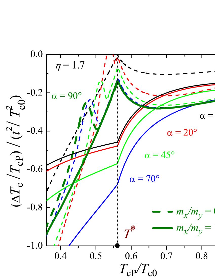
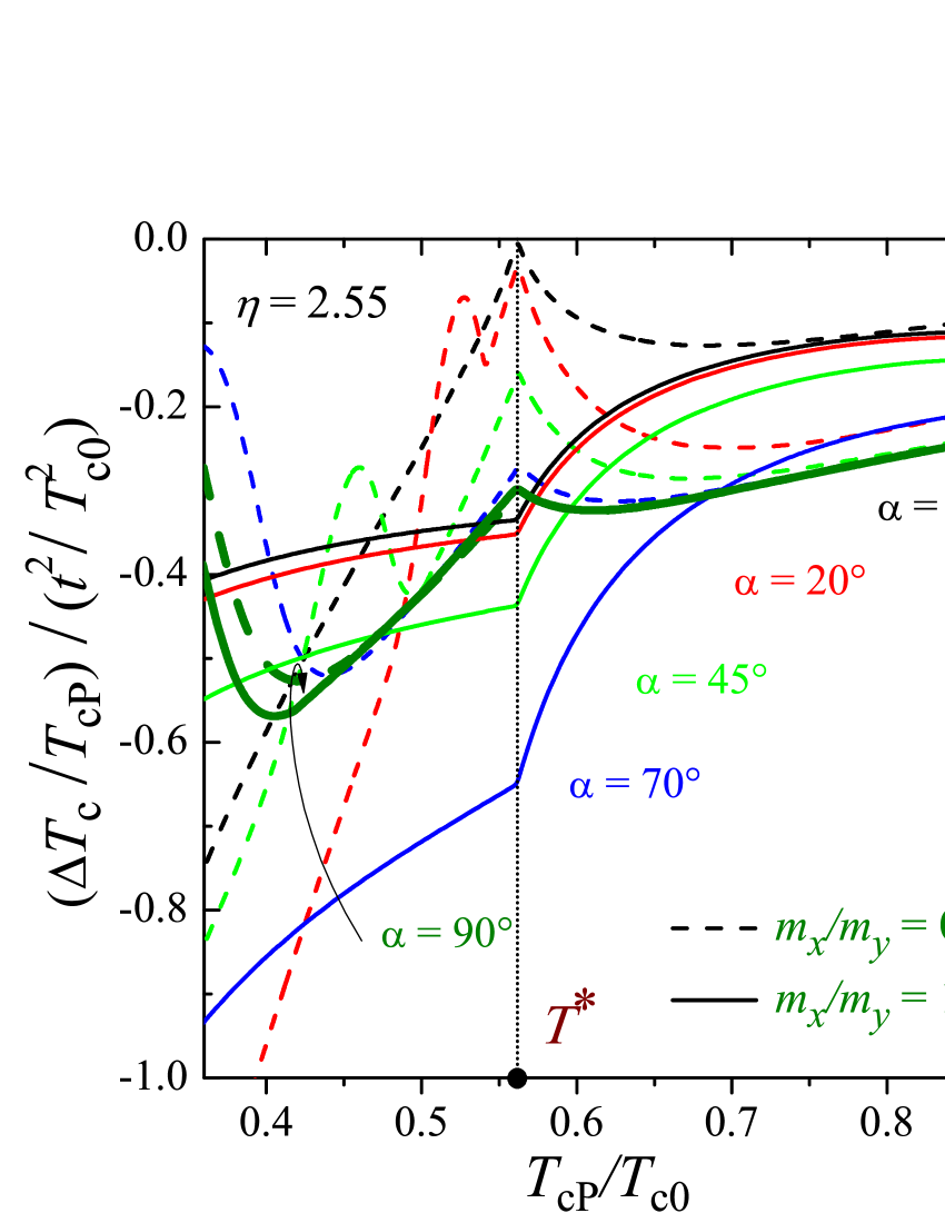
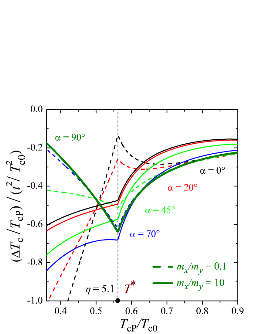
Figure 5: Contribution of the orbital effect as a function of $T_{cP}/T_{c0}$ for several angles $\alpha$ between $\mathbf{H}$ and $x$-axis, for $\eta=1.7$ (left panel), for $\eta=2.5$ (middle panel) , and for $\eta=5.1$ (right panel). Solid lines are the results obtained for $m_{x}/m_{y}=100$ and $m_{x}/m_{y}=10$; Dashed lines are for $m_{x}/m_{y}=0.01$, $m_{x}/m_{y}=0.1$.

Making use of the self-consistency relation the solution of the system of coupled equations (33 - 36) can be given in the form (for details see Appendix B)

$$\Delta_{0}\left[P+t^{2}a\right] =t^{2}\sum\limits_{\pm}c_{\pm}\Delta_{\mathbf{\pm}2},$$ (37)

$$\Delta_{\mathbf{+}2}\left[P+t^{2}b_{+}+\delta_{+}\right] =t^{2}c_{+}\Delta_{0},$$ (38)

$$\Delta_{\mathbf{-}2}\left[P+t^{2}b_{-}+\delta_{-}\right] =t^{2}c_{-}\Delta_{0}$$ (39)

where the following notations are introduced:

$$a =\pi T\sum\limits_{n,\xi=\pm}\left.T_{n}\left(\mathbf{q},\mathbf{q},\xi\mathbf{Q}\right)\right|_{T=T_{cP}},$$ (40)

$$b_{\pm} =\pi T\sum\limits_{n,\xi=\pm}\left.T_{n}\left(\mathbf{q}\pm 2\mathbf{Q},\mathbf{q}\pm 2\mathbf{Q},\mathbf{q}\pm 2\mathbf{Q+}\xi\mathbf{Q}\right)\right|_{T=T_{cP}},$$ (41)

$$c_{\pm} =\pi T\sum\limits_{n}\left.T_{n}\left(\mathbf{q},\mathbf{q}\pm\mathbf{Q},\mathbf{q}\pm 2\mathbf{Q}\right)\right|_{T=T_{cP}}$$ (42)

$$\delta_{\pm} =\pi T\sum\limits_{n}\left.\frac{1}{L_{n}\left(\mathbf{q}\right)}-\frac{1}{L_{n}\left(\mathbf{q}\pm 2\mathbf{Q}\right)}\right|_{T=T_{cP}}$$ (43)

with $T_{n}\left(\mathbf{q},\mathbf{p},\mathbf{k}\right)=\left\langle L_{n}^{-1}\left(\mathbf{q}\right)L_{n}^{-1}\left(\mathbf{p}\right)L_{n}^{-1}\left(\mathbf{k}\right)\right\rangle/2$. The solution of the system (37)-(38) is found from

$$\left|\begin{array}[]{ccc}P+t^{2}b_{-}+\delta_{-}&-t^{2}c_{-}&0\\ -t^{2}c_{-}&P+t^{2}a&-t^{2}c_{+}\\ 0&-t^{2}c_{+}&P+t^{2}b_{+}+\delta_{+}\end{array}\right|=0.$$ (44)

For $T>T^{\ast}$, when $q=0$, $\Delta_{\mathbf{+}2}=\Delta_{-2}$, which makes it possible to write the solution in the form

$$T_{c}=T_{cP}\left[1-AS^{\pm}\left(\mathbf{Q}\right)\right]$$ (45)

with

$$S^{\pm}\left(\mathbf{Q}\right)\equiv\frac{\left(a+b_{\pm}\right)t^{2}+\delta_{\pm}}{2}\\ +\frac{t^{2}}{2}\sqrt{\left[a-b_{\pm}-\delta_{\pm}/t^{2}\right]^{2}+4c_{\pm}\sum\limits_{\pm}c_{\pm}}.$$ (46)

If $\sqrt{tT_{c0}}\ll\hbar v_{F}Q$ then it further simplifies, $S^{\pm}\left(\mathbf{Q}\right)=at^{2}$. In Eq. (45) those values of $\pm$ are chosen that maximize the critical temperature. In general case, if $H<H^{\ast}$ then within a second-order approximation in the small parameter $t/T_{c0}$, $\Delta_{\mathbf{\pm}2}$ reads as

$$\Delta_{\mathbf{\pm}2}\approx\frac{t^{2}}{\left(\hbar v_{F}Q\right)^{2}}\Delta_{0}$$ (47)

and the solution (45) system (37-38) simplifies to (for details see Appendix C)

$$P=\pi T_{cP}\sum\limits_{n}\frac{t^{2}}{\Omega_{n}^{3}}\left[-1+\frac{1}{8}\frac{\left(\hbar v_{F}Q\right)^{2}}{\Omega_{n}^{2}}+\frac{t^{2}}{\left(\hbar v_{F}Q\right)^{2}}\right].$$ (48)

In the absence of the Zeeman effect

$$\ln\frac{T_{c}}{T_{ct}}=\frac{t^{2}}{\pi^{2}T_{c0}^{2}}\left[\frac{31\zeta\left(5\right)}{128}\frac{\left(\hbar v_{F}Q\right)^{2}}{\pi^{2}T_{c0}^{2}}+\frac{7\zeta\left(3\right)}{4}\frac{t^{2}}{\left(\hbar v_{F}Q\right)^{2}}\right].$$ (49)

which is the same as Eq. (26). Thus, within the expansion model (31) we obtained the upper critical field versus the superconducting onset temperature. This equation naturally describes the crossover between two regimes: the Lowerence-Doniach phase and the beginning of the Lebed re-entrant phase.

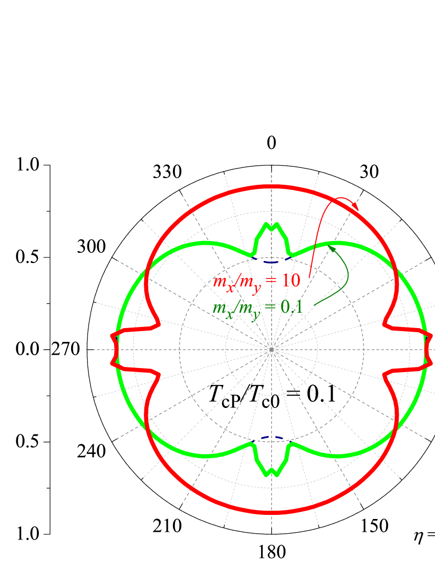
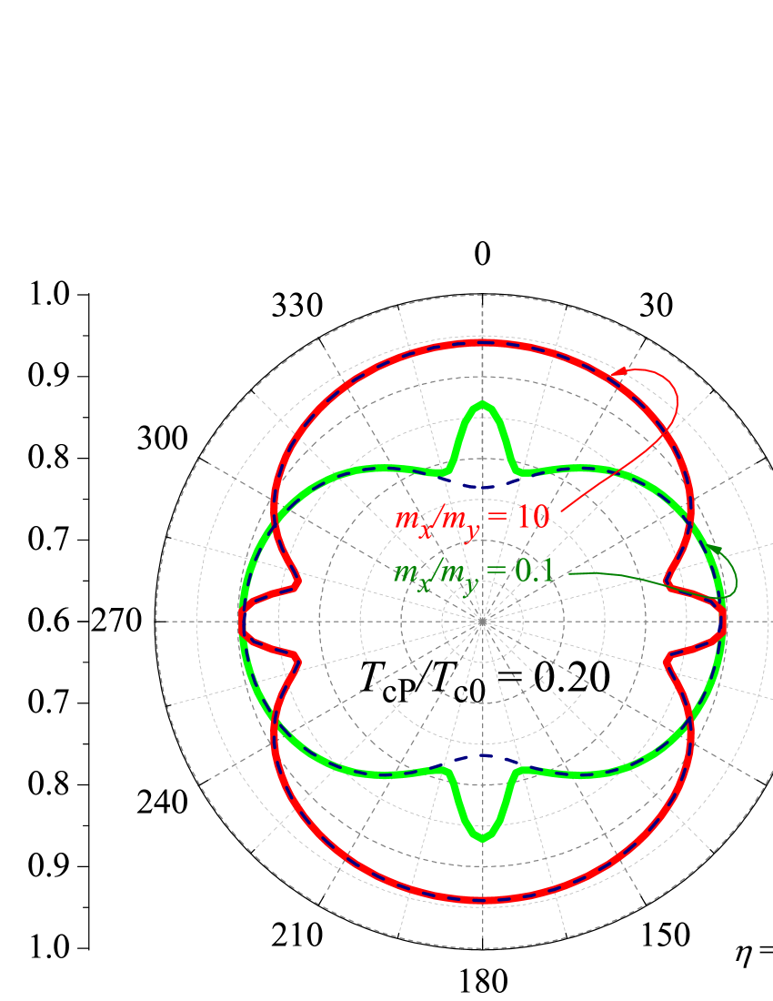
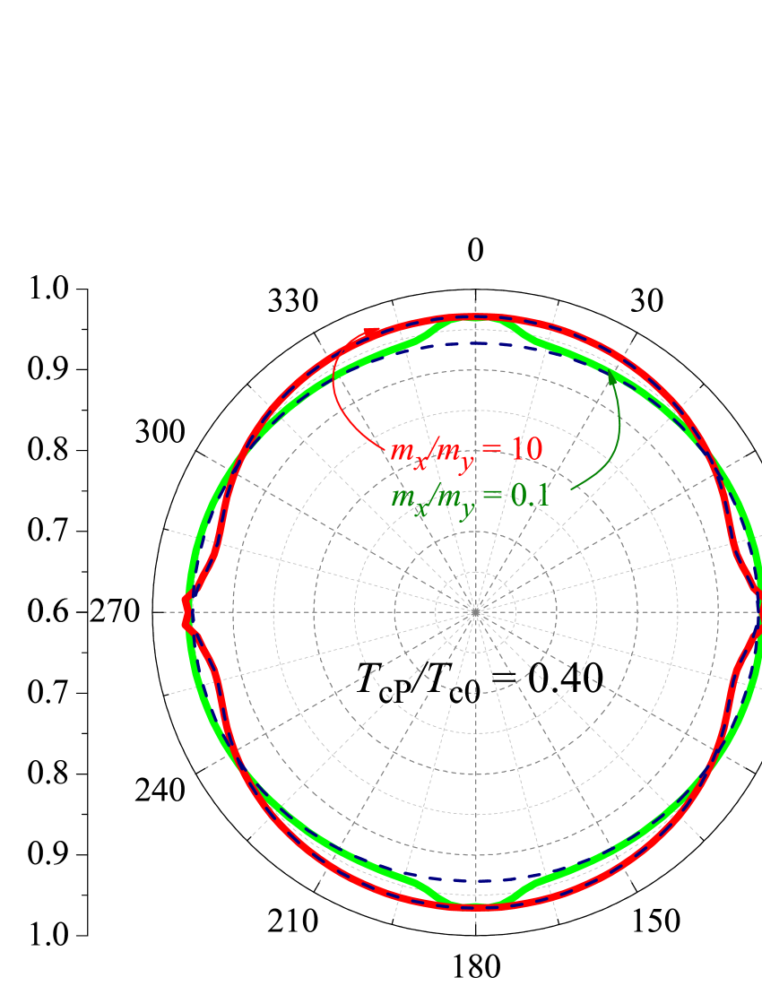
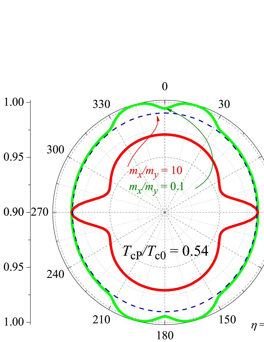
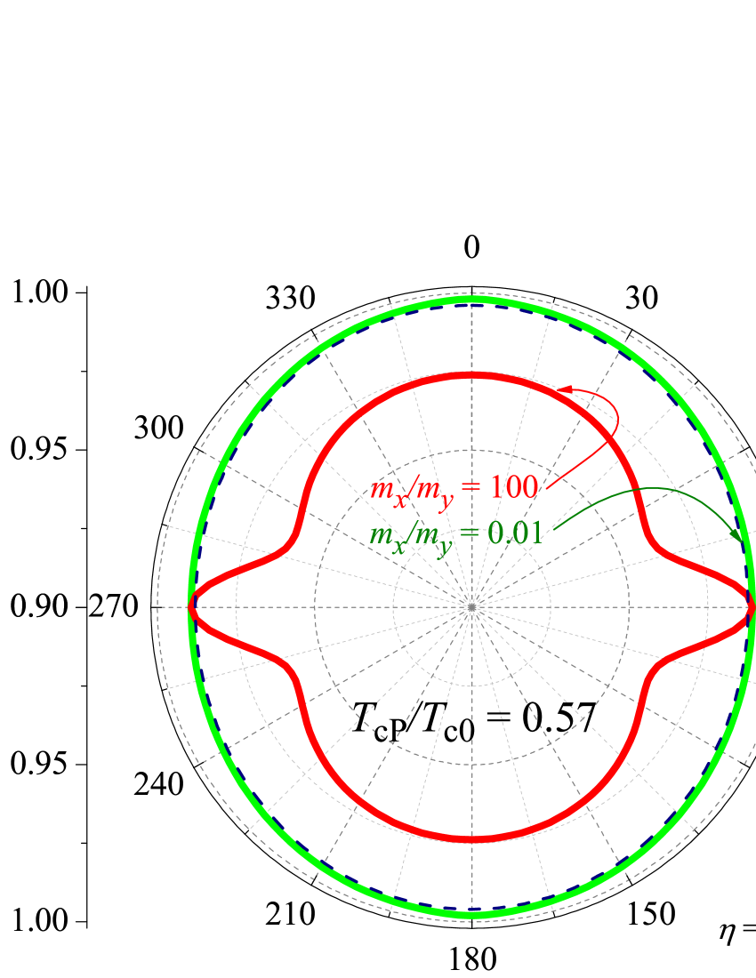
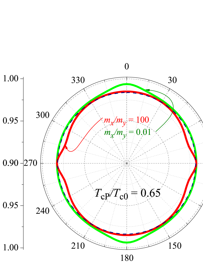
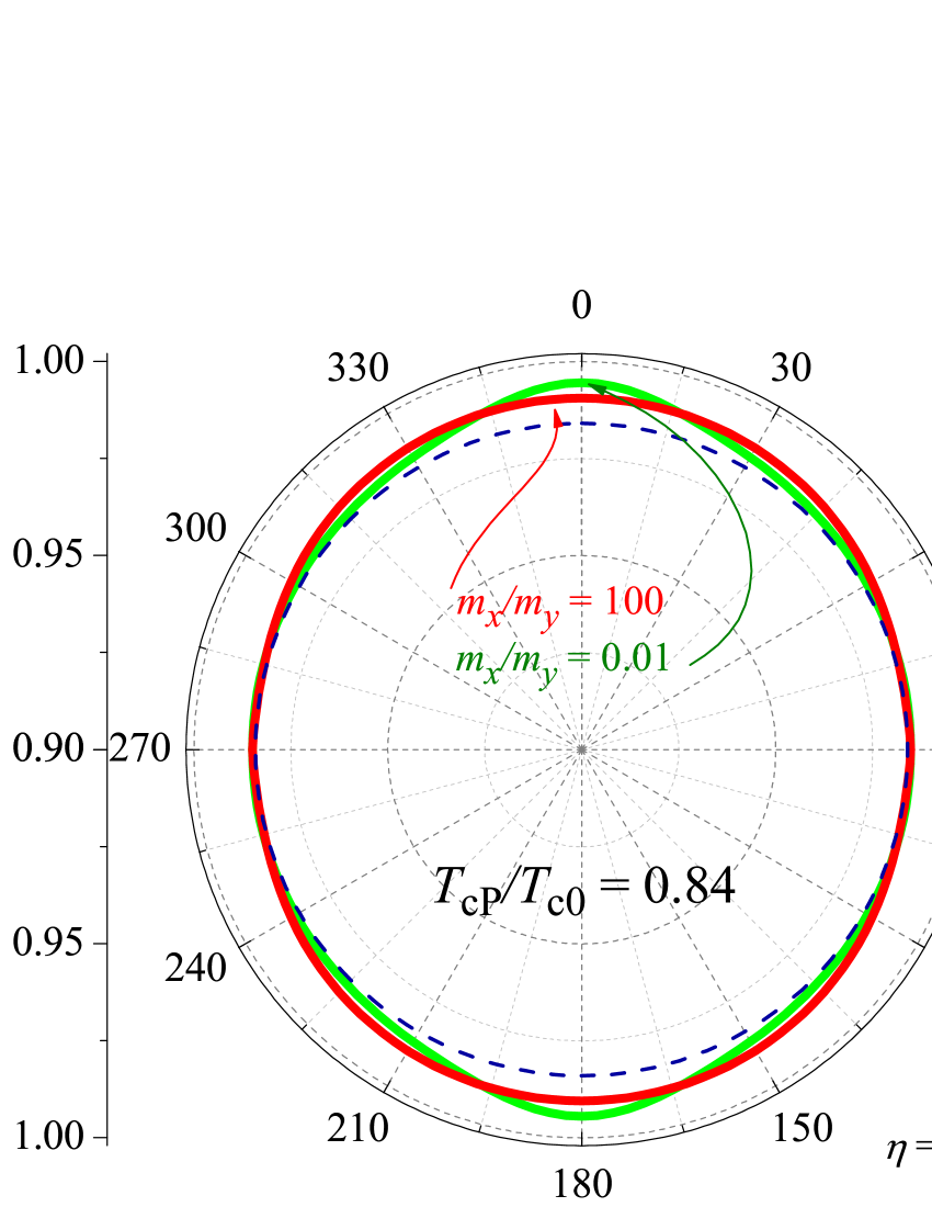
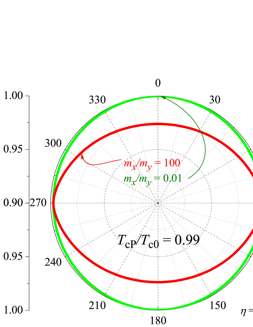
Figure 6: Normalized transition temperature, $T_{c}\left(\alpha\right)/T_{cP}$ as a function of $\alpha$ for several $T_{cP}/T_{c0}$, $t/T_{c0}=0.25$, and $\eta=1.7$. For the purpose of clarity the shown range of $T_{c}\left(\alpha\right)/T_{cP}$ is from 0.9 till 1.0. Dashed lines are for $\Delta_{\mathbf{\pm}2}\neq 0$.

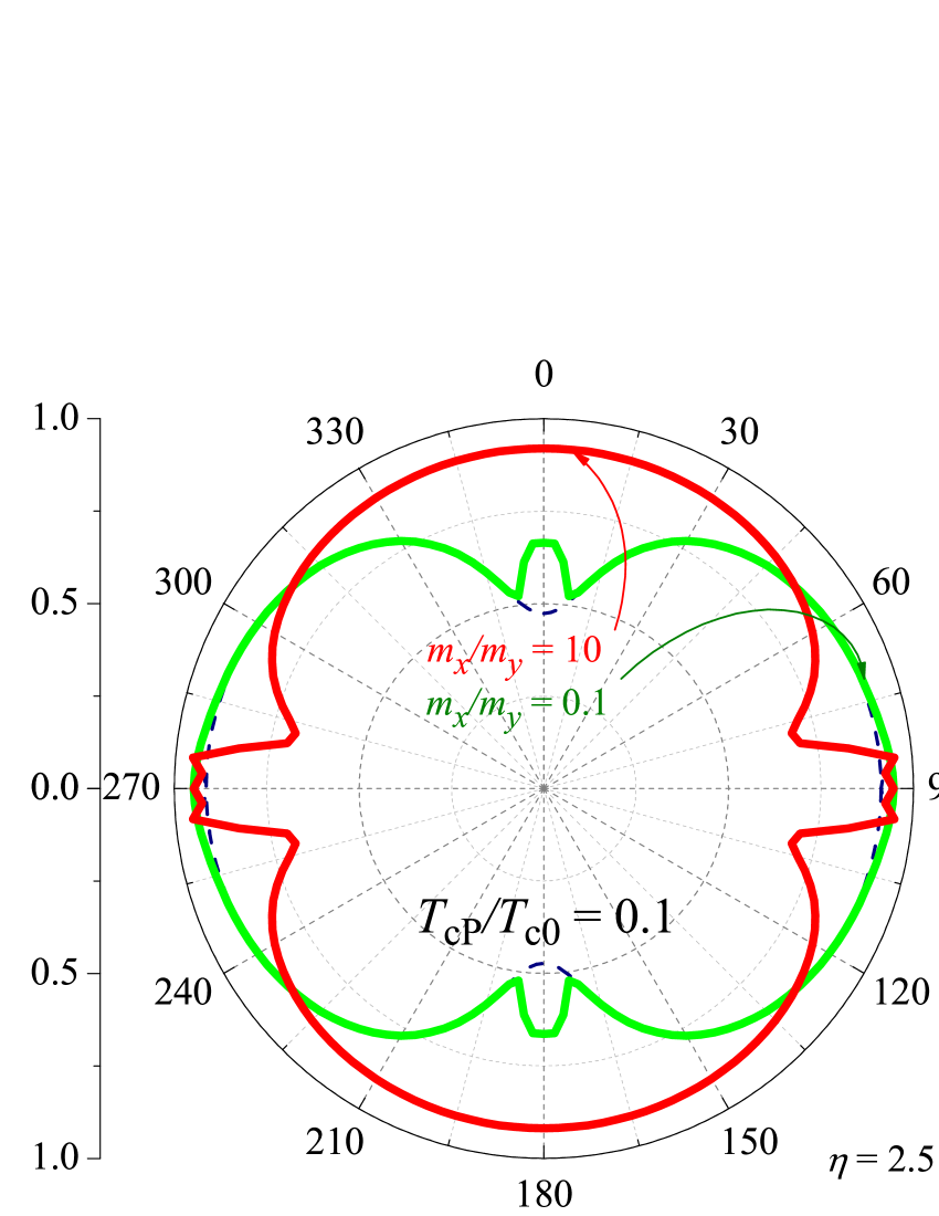
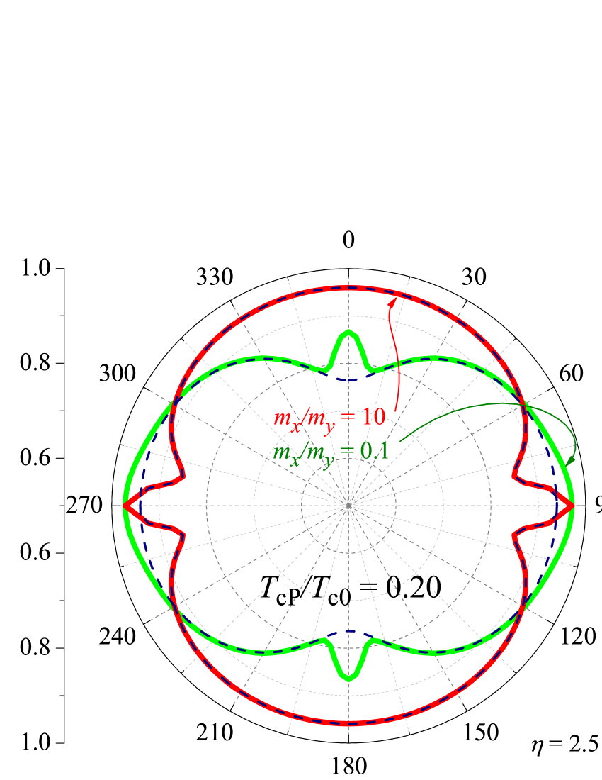
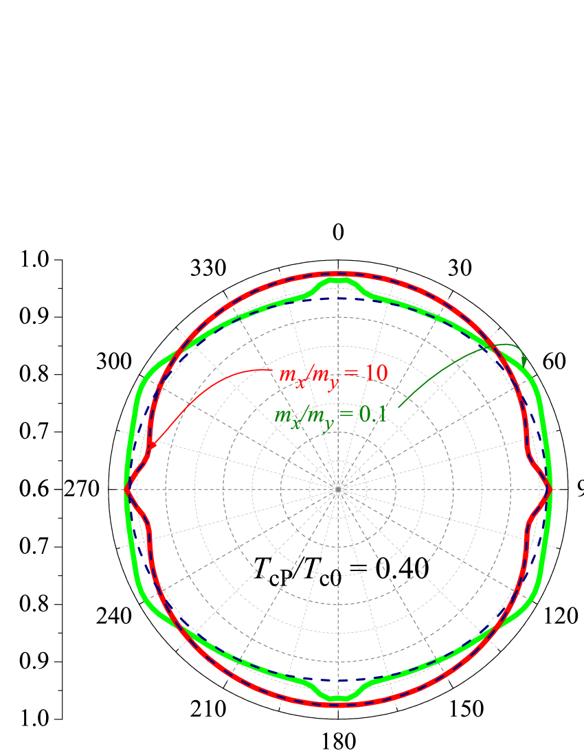
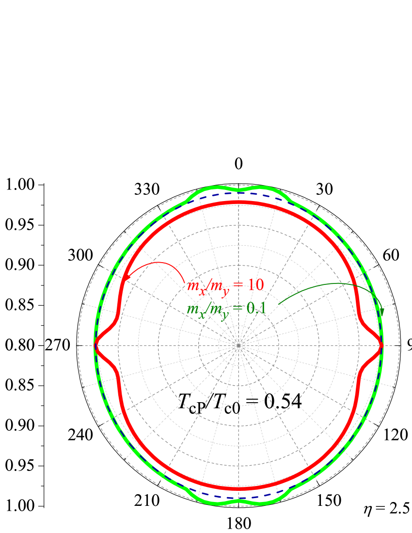
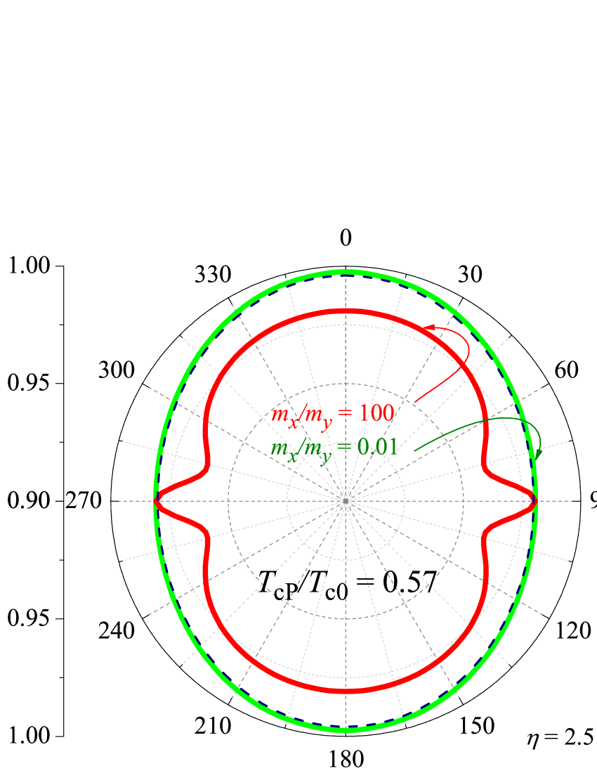
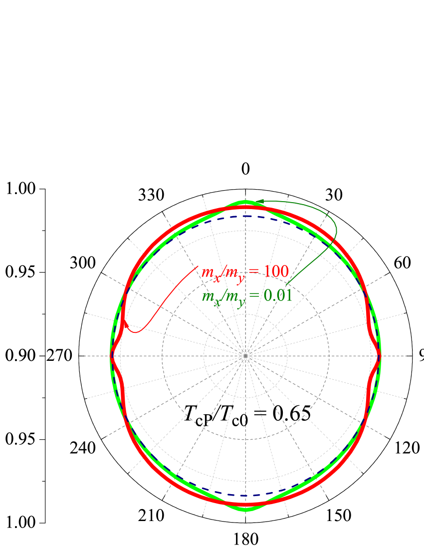
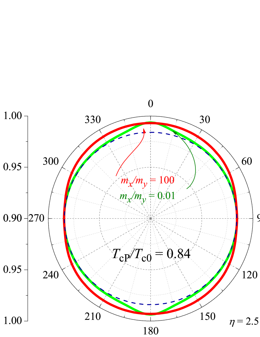
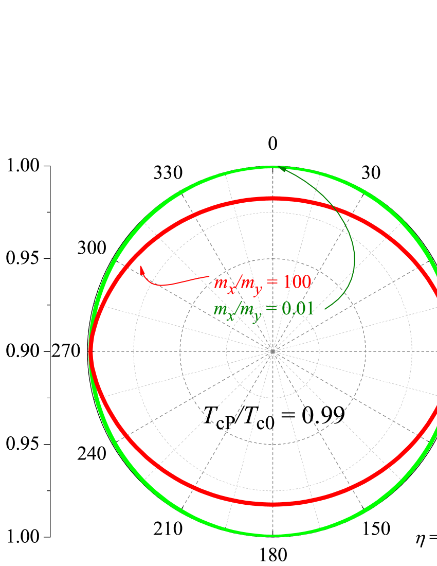
Figure 7: The same as in Fig. 5 but calculated for $\eta=2.5$, which corresponds to $v_{F}=7.5\times 10^{4}~{}\mathrm{m/\sec}$.

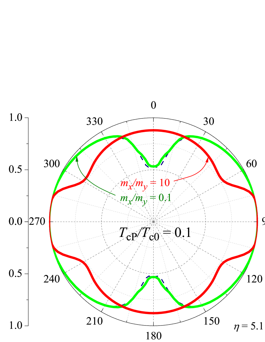
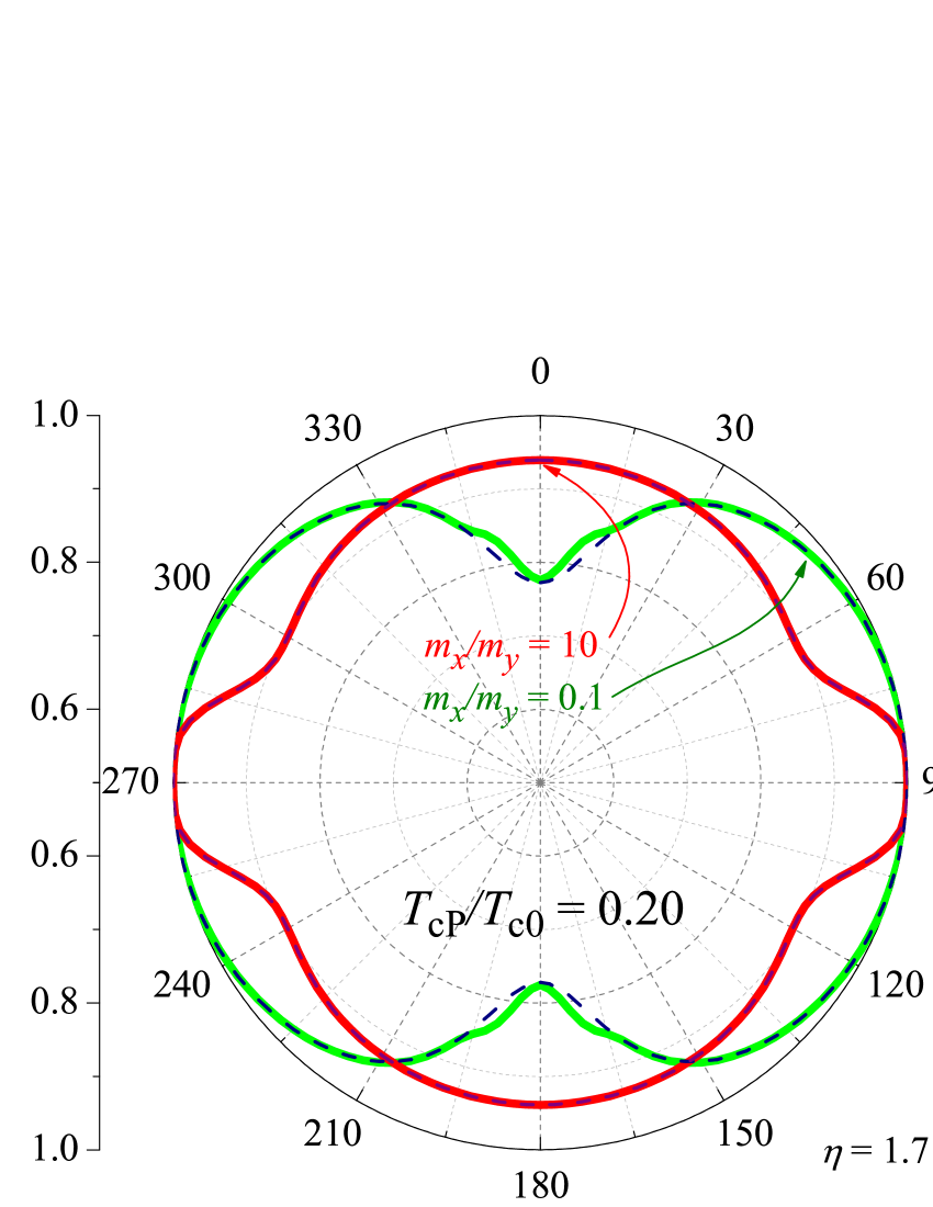
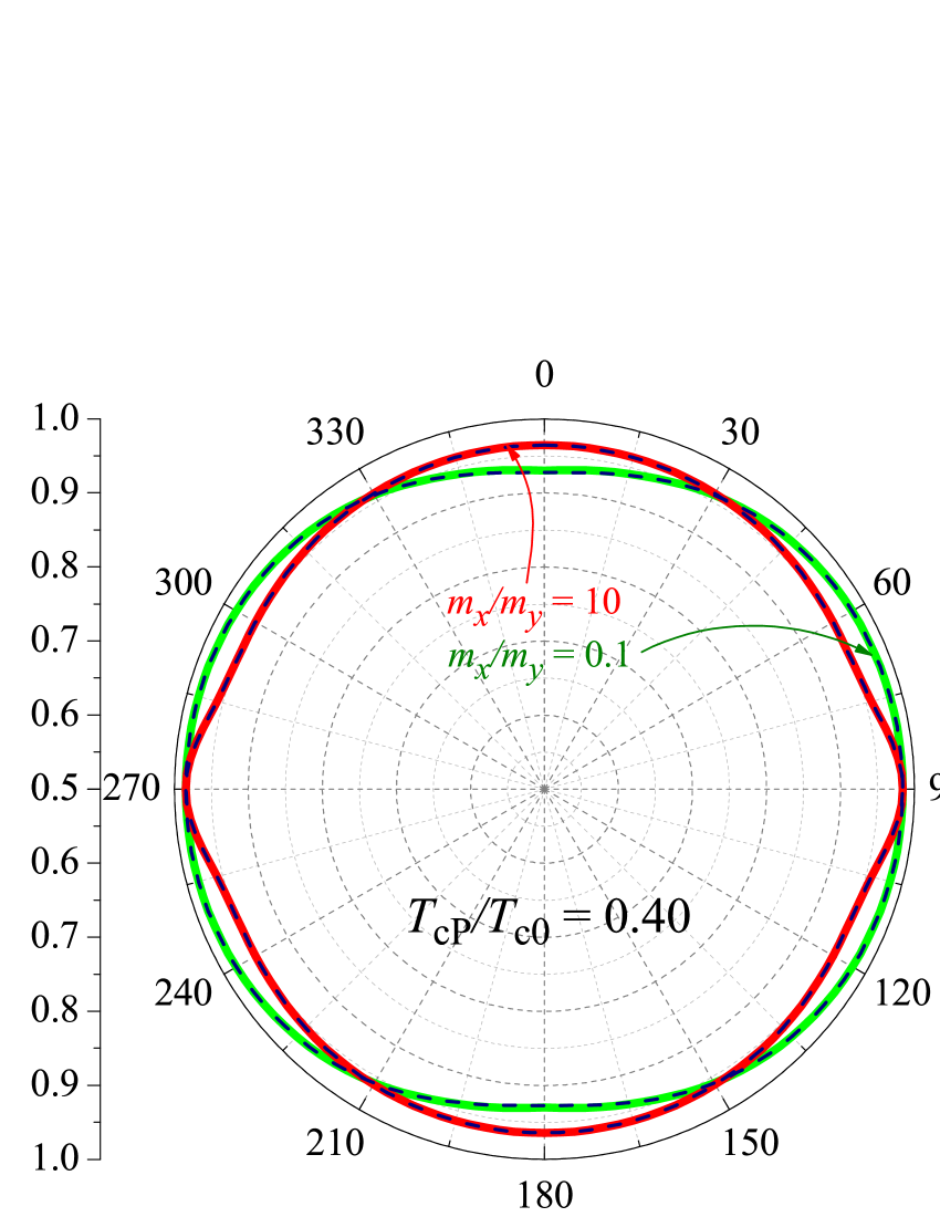
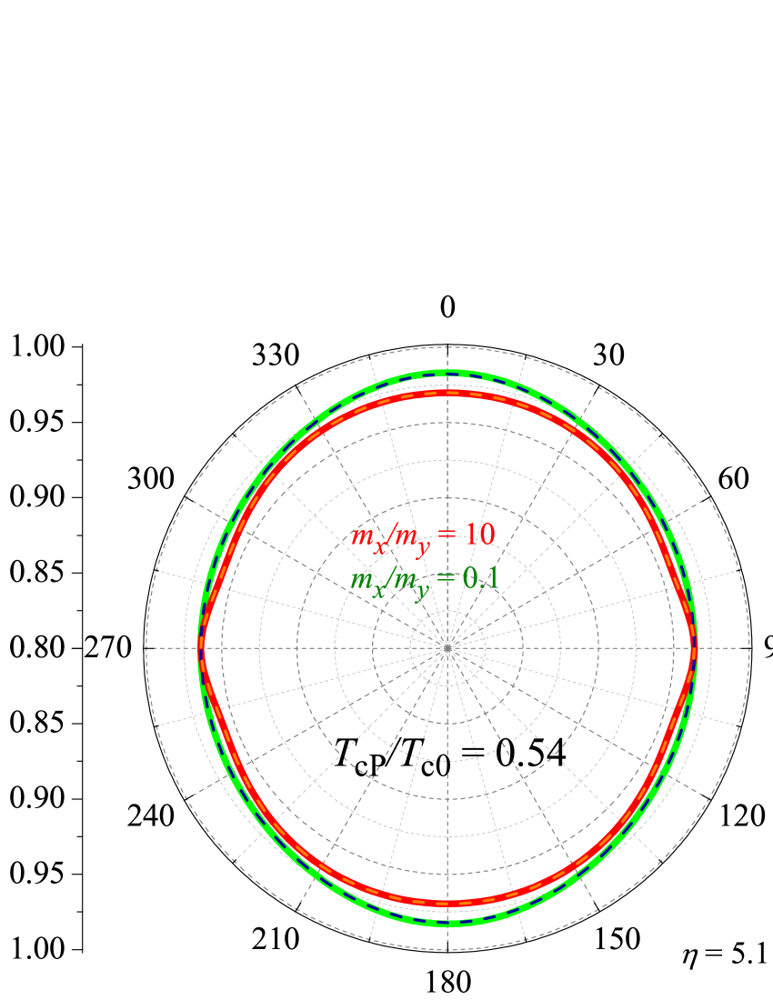
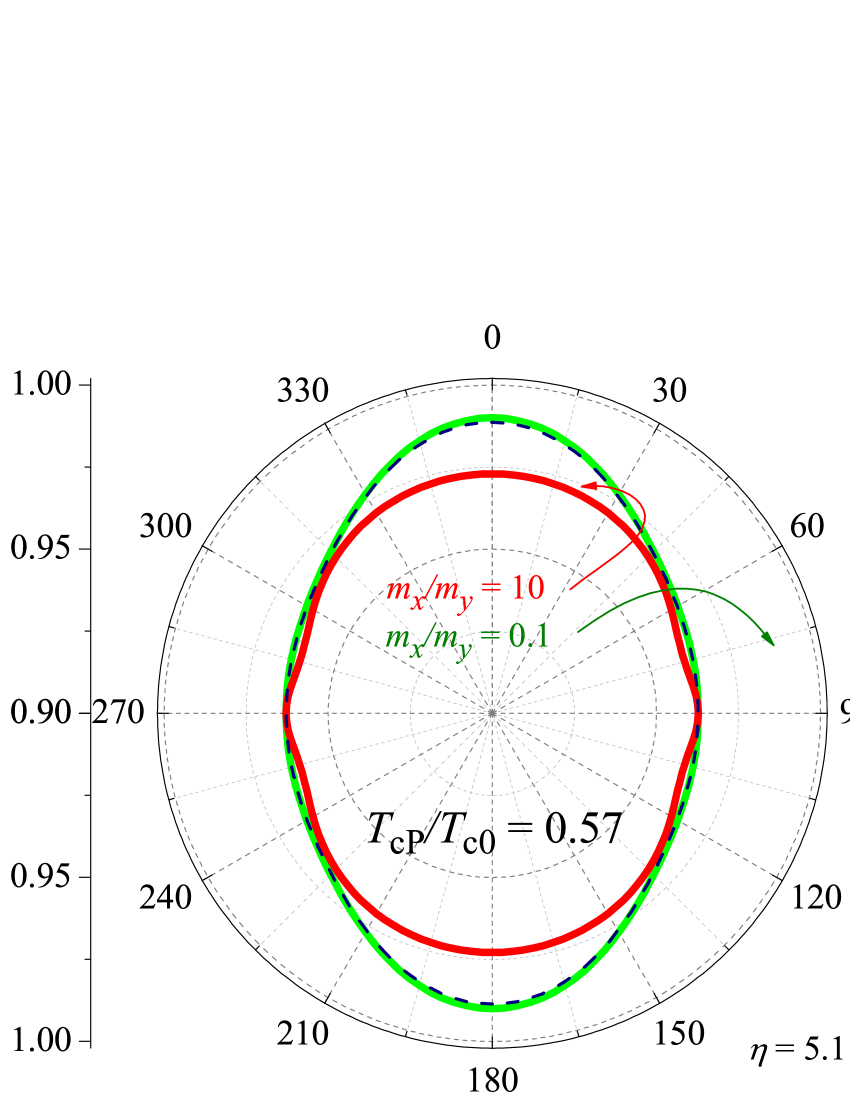
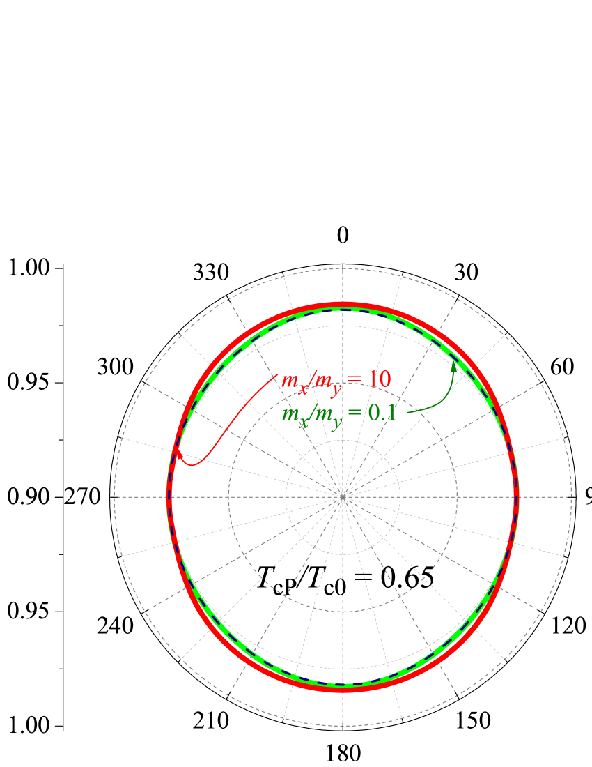
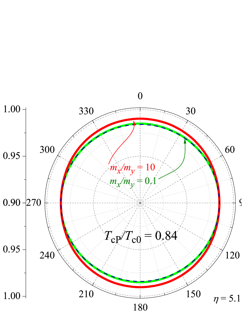
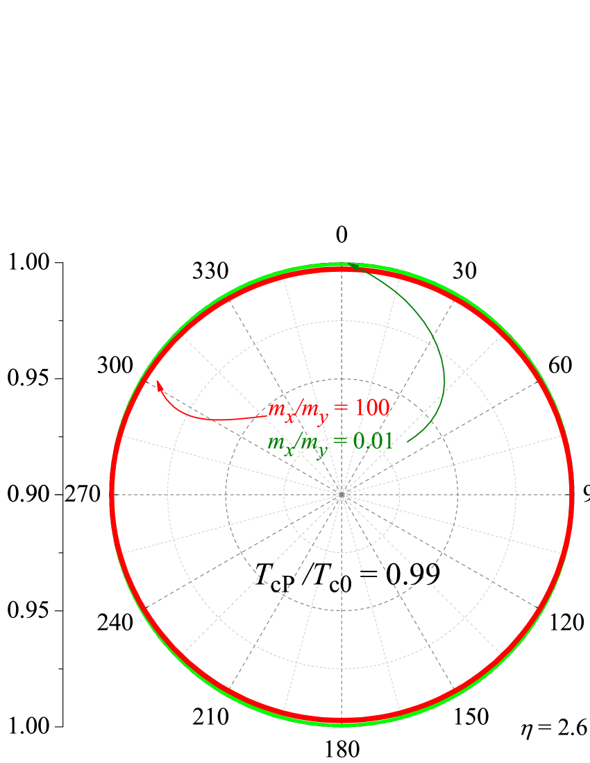
Figure 8: The same as in Fig. 5 but calculated for $\eta=5.1$, which corresponds to $v_{F}=1.5\times 10^{5}~{}\mathrm{m/\sec}$.

IV.0.1 Regime of high magnetic fields $\left(H\gg\frac{T_{c0}}{\pi\hbar dv_{F}}\phi_{0}\right)$

In the absence of the Zeeman effect, when studying the anisotropy of the upper critical field, such as $T_{c0}\ll\hbar v_{F}Q$, the second harmonics in the expansion Eq. (31) can be neglected, i.e. in Eq. (37) we set $\Delta_{\mathbf{\pm}2}=0$ and we get the following equation

$$\ln\frac{T_{c0}}{T_{c}}=\pi T_{c}\sum\limits_{n}\frac{t^{2}}{\omega_{n}}\frac{1}{\omega_{n}^{2}+\hbar^{2}\left(\frac{\mathbf{v}_{F}.\mathbf{Q}}{2}\right)^{2}}.$$ (50)

Performing average over the Fermi surface results in

$$\ln\frac{T_{c0}}{T_{c}}=\pi T_{c}\sum\limits_{n}\frac{t^{2}}{\omega_{n}^{2}}\frac{1}{\sqrt{\omega_{n}^{2}+\left(\hbar v_{F}Q\right)^{2}/4}}.$$ (51)

For extremely large magnitude of the external magnetic field we can simplify, since $\omega_{n}\sim$ $T_{c0}\ll v_{F}Q$

$$\ln\frac{T_{c0}}{T_{c}}=\frac{t^{2}}{\pi T_{c0}}\sum\limits_{n>0}\frac{1}{(n+\frac{1}{2})^{2}}\frac{1}{\hbar v_{F}Q}=\frac{\pi t^{2}}{2T_{c0}}\frac{1}{\hbar v_{F}Q}.$$ (52)

Therefore, the upper critical field is ($\varkappa_{IV}:$ $H\gg\frac{T_{c0}}{\pi\hbar dv_{F}}\phi_{0}$)

$$\left.H_{c2}^{h=0}\left(\frac{\pi}{2}\right)\right|_{\varkappa_{IV}}=\frac{t^{2}}{2\hbar dv_{F}}\frac{\phi_{0}}{\left(T_{c0}-T_{c}\right)}.$$ (53)

From Eq. 52 it is seen that an increase of the external field far beyond the value $\frac{T_{c0}}{\pi\hbar dv_{F}}\phi_{0}$ results in a critical temperature $T_{c}\rightarrow T_{c0}$. Hence at high magnetic fields the restoration of superconductivity is possible if the destruction of spin-singlet state of Cooper pairs may be neglected, as was predicted by Lebed.lebe01 lebe07 Therefore, we can infer that within our model the re-entrant phase of superconductivity is naturally described. Summarizing the above two sections we plot all considered regimes for the case of absence of the Zeeman effect in Fig. 3.

V Anisotropy of the upper critical field

In our numerical investigations we restrict ourselves to the following parameters: the interlayer coupling is $t=2.27$ K, $t/T_{c0}=0.25$, $\Delta_{0}=2.8kT_{c0}$mul and the Fermi velocity $v_{F}=5.0\times 10^{4}~{}\mathrm{m/\sec}$.iza Introducing the dimensionless Fermi velocity parameter, $\eta=\hbar v_{F}\pi d/\phi_{0}\mu_{B}$, this value of $v_{F}$ corresponds to $\eta=1.7$ and $d=1.62$ nm.bergk The summation over the Matsubara frequencies was performed numerically.

Fig. 4 shows the reduced temperature, $T_{cP}/T_{c0}$, dependence of the magnetic wave vector $\hbar Q_{c2}^{P}v_{F}/k_{B}T_{c0}$ for several values of the Fermi velocity parameter, when only the paramagnetic effect is accounted for. Here $Q_{c2}^{P}=\pi dH_{c2}^{P}/\phi_{0}$. The absolute value of the FFLO modulation wave vector is also given and it grows from zero for $T<T^{\ast}$. To highlight the contribution of the orbital correction to the superconducting onset temperature, obtained in the paramagnetic limit, $\Delta T_{cP}=T_{c}-T_{cP}$, and how it depends on the magnitude of the external magnetic field applied parallel to the conducting planes we performed calculations with Eq. (45). Fig. 5 displays the normalized orbital correction, $\Delta T_{cP}/T_{cP}$, as a function of reduced temperature for several angles $\alpha$ that the external field makes from the x-axis. The left and middle panels display the results for the velocity parameter $\eta=1.7$ and $\eta=2.55$, respectively. The solid lines correspond to the in-plane mass anisotropy $m_{x}/m_{y}=100$, while the dashed lines display the results for $m_{x}/m_{y}=0.01$. The right panel illustrates the results for $\eta=5.1$, $m_{x}/m_{y}=10$ (solid lines), $m_{x}/m_{y}=0.1$ (dashed lines). One can distinguish the in-plane mass anisotropy from the temperature dependence of the orbital corrections for angles $\alpha\neq\pm 90{{}^{\circ}}$. For example, for $m_{x}/m_{y}=100$ a decrease of temperature from $T\lesssim 0.9T_{c0}$, or an increase of the applied magnetic field from $H\gtrsim 0.1H_{P0}$, first exhibits a weak influence on $\Delta T_{cP}/T_{cP}$, but when $T\lesssim 0.65T_{c0}$ ($H\gtrsim 0.5H_{P0}$. Here $H_{P0}=\Delta_{0}/\mu_{B}$ is the critical magnetic field at $T=0$ in Pauli limited 2D superconductors) it gradually increases $\left|\Delta T_{cP}\right|$, i.e. the orbital suppression of superconductivity becomes stronger with magnetic field, when orbital pair-breaking is superimposed on the spin pair breaking mechanism. For $m_{x}/m_{y}=0.01$ an increase of the applied field results first in a progressive increase of $\left|\Delta T_{cP}\right|$. However, for $T\lesssim 0.65T_{c0}$ we see an opposite bias, namely strengthening of the applied field rapidly reduces $\left|\Delta T_{cP}\right|$, i.e. the orbital pair breaking becomes weaker with the external field, and it can almost vanish for some directions of the field in the very close vicinity of the tricritical point as seen for dashed curves $\alpha=0$. For $\alpha=90{{}^{\circ}}$ the curves describing $m_{x}/m_{y}=100$ mass anisotropy coincide with those for $m_{x}/m_{y}=0.01$ and both follow the tendency typical for $m_{x}/m_{y}=0.01$ mass anisotropy. In Fig. 5 both curves are given by the thick lines. We can also infer that an increase of the Fermi velocity weakens this effect of $\left|\Delta T_{cP}\right|$ reduction as seen from the middle panel of Fig. 5. In the FFLO phase, for $T<T^{\ast}$, or $H>H^{\ast}$, the orbital correction in both cases of mass anisotropy essentially increases, especially for $m_{x}/m_{y}=0.01$ and for some angles can show a non-monotonic behavior. The further increase of the Fermi velocity can modify the just described behavior. Indeed, as seen from the right figure the $\alpha=90{{}^{\circ}}$ curves follow the tendency typical for $m_{x}/m_{y}=10$ mass anisotropy and in the FFLO phase they show an upturn.

Opposite tendency in the field direction dependence of the normalized correction, $\Delta T_{cP}$, for the range of angles $\alpha=0{{}^{\circ}}-$ $70{{}^{\circ}}$ and for the angles in the close vicinity of $\alpha=90{{}^{\circ}}$ in the case of $m_{x}/m_{y}=100$ should result in a particular anisotropy of the onset of superconductivity. Figs. 6 and 7 show the magnetic field angular dependence of the normalized superconducting transition temperature, $T_{c}\left(\alpha\right)/T_{cP}$, calculated at $T_{cP}/T_{c0}\simeq 0.1$, $0.2$, $0.4$, $0.54$, $0.57$, $0.65$, $0.84$ and $0.99$ for the velocity parameter $\eta=1.7$ and $\eta=2.55$, respectively. In the polar plot the direction of each point seen from the origin corresponds to the magnetic field direction and the distance from the origin corresponds to the normalized critical temperature. We see that for $m_{x}/m_{y}=100$ the reduction of the orbital suppression of superconductivity at $\alpha=\pm 90{{}^{\circ}}$ in the vicinity of the tricritical point is accompanied by a grow of cusps at these angles in the field-angle dependence of $T_{c}\left(\alpha\right)/T_{cP}$. The cusps appear at $Q\|Ox$, i.e. magnetic field is along the light mass direction, as intuitively expected, since it is more difficult to induce diamagnetic currents with heavier charge carriers. For $m_{x}/m_{y}=0.01$ the overall orbital corrections are smaller than that for $m_{x}/m_{y}=100$. This is due to the fact that in the former case the Fermi surface is smaller and hence the diamagnetic response is weaker than that in the latter situation. In $\frac{ig.}{{}}$8 $T_{c}\left(\alpha\right)/T_{cP}$ is shown for $\eta=5.1$ and $m_{x}/m_{y}=10$ (red lines), $m_{x}/m_{y}=0.1$ (green lines). Formation of cusps in the vicinity of the tricritical point is also observed, although to a smaller extent. In Figs. 6, 7 and 8 the dashed lines are $T_{c}\left(\alpha\right)/T_{cP}$ obtained for $m_{x}/m_{y}=0.01$($0.1$ in Fig. 8) when the r.h.s. of Eq. (37) is neglected, $\Delta_{\mathbf{\pm}2}=0$. In this case the solution (45) simplifies to

$$T_{c}=T_{cP}\left[1-At^{2}a\right]$$ (54)

and such solution is valid for $\sqrt{tT_{c0}}\ll\hbar v_{F}Q$, which is the beginning of the superconductivity re-entrant regime.lebe01 ; lebe06 As the charge carrier mass becomes smaller the superconducting re-entrant phase begins at a higher magnetic field. Since, according to Eq. (74) the second harmonics of the order parameter generates the Lowerence-Doniach term in the original expression, Eq. (78), the dashed lines give a hint about its contribution to the in-plane anisotropy of the onset of superconductivity in layered structures with $m_{x}/m_{y}=0.01$ in-plane mass anisotropy. We see that the difference between the solutions (45) and (54) is negligible for $T_{cP}/T_{c0}\simeq 0.57$. However it is noticeable already for $T_{cP}/T_{c0}\simeq 0.65$. The upper and lower knobs are observed when the full original expression is used, and they are absent for the simplified version, Eq. (54). So we can infer that the observed knobs are due to the Lowerence-Doniach term. Because this term becomes less important with the field, the knobs are absent for $T_{cP}/T_{c0}\simeq 0.57$ and essentially pronounced for $T_{cP}/T_{c0}\simeq 0.85$, when $m_{x}/m_{y}=0.01$. Inversely, for $m_{x}/m_{y}=100$ the cusps are profound near the tricritical point, insignificant for smaller fields, and essentially seen far beyond the tricritical point in the FFLO phase. The cusps are induced by the $t^{2}a$-term, which in the conventional phase acquires the following form

$$at^{2}=\pi T_{cP}\sum\limits_{n}\frac{t^{2}}{\Omega_{n}^{3}}\frac{1}{\sqrt{1+\varepsilon\left(\mathbf{Q}\right)/2\Omega_{n}^{2}}}$$ (55)

From Fig. (7) we can infer that an increase of the Fermi velocity leads to a narrowing of the cusp width. However such increase of the Fermi velocity makes the cusps less pronounced.

In the FFLO phase $\hbar v_{F}Q\gtrsim T_{c0}$, and the solution Eq. (54) can be used for calculations. The top panels of Figs. 6, 7 and 8 illustrate the anisotropy of the superconducting onset temperature in the FFLO phase. We see that the cusps induced by the $t^{2}a$-term becomes even more profound with the magnetic field. Moreover, for $m_{x}/m_{y}=0.01$ a difference between the results obtained within $\Delta_{\mathbf{\pm}2}\neq 0$ and $\Delta_{\mathbf{\pm}2}=0$ appears. For $m_{x}/m_{y}=0.1$ this discrepancy is also present, although less visible. As was shown and explained in Ref. vrnkch02 this deviation this time is due to the resonance between FFLO modulation wave vector and the interlayer coupling modulated by the vector potential. Thus, in addition to the overall anisotropy induced by the FFLO modulation and studied in Ref. vrnkch01 , additional cusps develop for certain directions of the applied field, when the resonance conditions are realized. To describe resonances we have to account for the second harmonics, $\Delta_{\mathbf{\pm}2}$, and then

$$S^{\pm}\left(\mathbf{Q}\right)\equiv\frac{\left(a+b_{\pm}\right)t^{2}+\delta_{\pm}}{2}\\ +\frac{t^{2}}{2}\sqrt{\left[a-b_{\pm}-\delta_{\pm}/t^{2}\right]^{2}+4c_{\pm}^{2}}.$$ (56)

In general, in the vicinity of the tricritical point when comparing the in-plane anisotropy of $T_{c}\left(\alpha\right)$ for the conventional phase with that in the FFLO modulated phase, $T<T^{\ast}$ or $H>H^{\ast}$,vrnkch01 it is obviously seen a significant discrepancy. On both sides of the tricritical point, $T^{\ast}$, the contribution of the $t^{2}a$-term is essential and the observed difference is purely induced by the appearance of the FFLO modulation wave vector.

The anisotropy of the onset of superconductivity obtained within our model for $t\ll\hbar v_{F}Q$ and $m_{x}/m_{y}=100$ qualitatively similar to that observed in the experiment with (TMTSF)₂ClO₄.yone01 For $H<H^{\ast}$ our theoretical calculations show that in $T_{c}\left(\alpha\right)/T_{cP}$ cusps develop along the light masses. The same cusps and along the this direction are visible for $H=20$ kOe and $H=25$ kOe in the experimental data for $T_{c}\left(\alpha\right)/T_{cP}$. Our calculations show that for $H>H^{\ast}$ small dips appear from both sides of each cusp. Similar picture is observed in the experiment for $H>30$ kOe.

If we compare the field-direction dependence of the superconducting onset temperature for $T_{cP}/T_{c0}\lesssim 0.85$, valid for $\hbar v_{F}Q$ $\gg t$, with that in the last panels of Figs. 6, 7 and 8, where the result of the Ginzburg-Landau regime Eq. (18), valid for $\hbar v_{F}Q$ $\ll t$, is shown at $T_{cP}/T_{c0}\simeq 0.99$ we see an essential distinction. In the vicinity of $T_{c0}$ the anisotropy of the onset of superconductivity shows a typical picture for the anisotropic Ginzburg-Landau model. $T_{c}\left(\alpha\right)$ is maximum for $\mathbf{H}\bot Ox$ near $T_{c0}$ and as seen from Fig. 6 also in the vicinity of $T^{\ast}$.

VI Conclusions

In this work we have derived the extended Lawrence-Doniach model, which allows one to study superconductivity of layered materials at high magnetic fields. Within this model we have analyzed the field-amplitude and the field-direction dependence of the onset of superconductivity in layered conductors. Our theoretical analysis gives rise to the following assertion. There are four regimes, which we discriminate according to the distinctive features of the anisotropy of the onset of superconductivity and the temperature dependence of the upper critical field. (i) In the Ginzburg-Landau regime, when $H\ll\frac{t}{\pi\hbar dv_{F}}\phi_{0}$, $\left.H_{c2}\right|_{GL}\sim\left(T_{cP}-T_{c}\right)$, the anisotropy is well described within the continuous GL model. (ii) In the Lowerence-Doniach regime, within $t\phi_{0}/\pi\hbar dv_{F}\ll H\ll\sqrt{tT_{c0}}\phi_{0}/\pi\hbar dv_{F}$, $\left.H_{c2}\right|_{LD}\sim 1/\sqrt{\left(T_{c}-T_{ct}\right)}$, the anisotropy is mostly determined by the term proportional to $t^{4}/\left(\hbar v_{F}Q\right)^{2}$, which induces knobs in the direction along the light masses in the field-angle dependence of $T_{c}\left(\alpha\right)$. (iii) For $\frac{\phi_{0}}{\pi\hbar dv_{F}}\sqrt{tT_{c0}}\ll H\ll\frac{\phi_{0}}{\pi\hbar dv_{F}}T_{c0}$, $\left.H_{c2}\right|_{RS}=\sqrt{\left(T_{c}-T_{ct}\right)}$, the anisotropy is governed by the $t^{2}a$-term, which is responsible for the re-entrant of superconductivity. (iv) the FFLO phase, $H>H^{\ast}$, the anisotropy is settled by the interplay between the modulation and magnetic field wave vectors. The third regime can be deep in the four one so the discussed cusps can be invisible in the conventional phase. The paramagnetic effect is crucial for the description of the upper critical field both above and below the tricritical point. If the paramagnetic effect is negligible than the extended Lowerence-Doniach model restores the re-entrant behavior with magnetic field originally obtained by Lebed.lebe01 ; lebe06

Near $T_{c0}$ the anisotropy of the onset of superconductivity shows the smooth variation of $T_{c}\left(\alpha\right)$. When reducing the temperature, above the tricritical point small cusps appear. We may expect that small cusps observed in the field-direction dependence of $T_{c}\left(\alpha\right)/T_{cP}$ in the experiment with (TMTSF)₂ClO₄ near the Pauli limiting field, $H_{P0}=26$ kOeyone01  could have the re-entrant phase origin and are well described by the extended Lawrence-Doniach model. A technique that control the anisotropy of the upper critical field can provide an invaluable tool for investigating the physical origin of the experimentally observed upturn of the upper critical field in the low temperature regime.

Appendix A Derivation of the expression for A.

Substitution of Eq. (13) in Eq. (10) results in

$$\Delta\left(\mathbf{r},k_{z}\right)\ln\frac{T_{c}}{T_{cP}}=\Delta\left(\mathbf{r},k_{z}\right)\\ \times\left[F\left(\frac{h}{\pi T_{c}}\right)-F\left(\frac{h}{\pi T_{cP}}\right)\right]+\widehat{\Pi}_{\mathrm{MLD}}\Delta\left(\mathbf{r},k_{z}\right),$$ (57)

where we defined a function

$$F\left(\frac{h}{\pi T}\right)\equiv\pi T\sum\limits_{n}\left[\frac{1}{\omega_{n}\left(T\right)}-\frac{1}{\Omega_{n}\left(T\right)}\right].$$ (58)

When expanding in series, taking into account that $\left(T_{c}-T_{cP}\right)/T_{c}\ll 1$ we obtain

$$\Delta\left(\mathbf{r},k_{z}\right)\frac{T_{c}-T_{cP}}{T_{c}}=\Delta\left(\mathbf{r},k_{z}\right)\frac{h}{\pi T_{cP}}\frac{T_{c}-T_{cP}}{T_{c}}\\ \times\frac{\partial}{\partial\left(\frac{h}{\pi T}\right)}\left.F\left(\frac{h}{\pi T}\right)\right|_{T=T_{cP}}+\widehat{\Pi}_{\mathrm{MLD}}\Delta\left(\mathbf{r},k_{z}\right),$$ (59)

and hence

$$\Delta\left(\mathbf{r},k_{z}\right)\frac{T_{c}-T_{cP}}{AT_{c}}=\widehat{\Pi}_{\mathrm{MLD}}\Delta\left(\mathbf{r},k_{z}\right),$$ (60)

where we introduced the following notations

$$P=\frac{T_{c}-T_{cP}}{AT_{c}},$$ (61)

and $A$ is given by

$$A^{-1}=1-\frac{h}{\pi T}\frac{\partial}{\partial\left(\frac{h}{\pi T}\right)}\left.F\left(\frac{h}{\pi T}\right)\right|_{T=T_{cP}}.$$ (62)

Appendix B Derivation of Eqs. (37-39)

Solution of the system of coupled equations (33 - 36) can be found as follows. From Eq. (36) we find

$$f_{\pm 3}=\mp\frac{\widetilde{t}f_{\pm 2}}{L_{n}\left(\pm 3\mathbf{Q}\right)}$$ (63)

and substituting it into Eq. (35) gives

$$\left[L_{n}\left(\pm 2\mathbf{Q}\right)+\frac{t^{2}}{L_{n}\left(\pm 3\mathbf{Q}\right)}\right]f_{\pm 2}\pm\widetilde{t}f_{\pm 1}=\Delta_{\mathbf{\pm}2}.$$ (64)

Then substitution of $f_{\pm 1}$, obtained from Eq. (34),

$$f_{\pm 1}=\mp\frac{\widetilde{t}f_{0}}{L_{n}\left(\pm\mathbf{Q}\right)}\mathbf{\pm}\frac{\widetilde{t}f_{\pm 2}}{L_{n}\left(\pm\mathbf{Q}\right)},$$ (65)

when taking into account that within the required approximation $f_{0}\approx\Delta_{0}/L_{n}\left(\mathbf{q}\right)$, produces the equation for the second harmonic of the pair amplitude, $f_{\pm 2}$,

$$\left[L_{n}\left(\pm 2\mathbf{Q}\right)+\frac{\widetilde{t}^{2}}{L_{n}\left(\pm 3\mathbf{Q}\right)}+\frac{\widetilde{t}^{2}}{L_{n}\left(\pm\mathbf{Q}\right)}\right]f_{\pm 2}\\ -\frac{\widetilde{t}^{2}\Delta_{0}}{L_{n}\left(0\right)L_{n}\left(\pm\mathbf{Q}\right)}=\Delta_{\mathbf{\pm}2}.$$ (66)

Substitution of $f_{\pm 1}$ from Eq. (65) and $f_{\pm 2}\approx\Delta_{\pm 2}/L_{n}\left(\mathbf{q}\pm 2\mathbf{Q}\right)$, obtained within the required approximation from Eq. (66), into Eq. (33) results in the following equation for $f_{0}$

$$\left[L_{n}\left(0\right)+\frac{\widetilde{t}^{2}}{L_{n}\left(+\mathbf{Q}\right)}+\frac{\widetilde{t}^{2}}{L_{n}\left(-\mathbf{Q}\right)}\right]f_{0}\\ -\sum\limits_{\pm}\frac{\widetilde{t}^{2}\Delta_{\mathbf{\pm}2}}{L_{n}\left(\pm\mathbf{Q}\right)L_{n}\left(\pm 2\mathbf{Q}\right)}=\Delta_{0}.$$ (67)

Since we adopt a second-order approximation in the small parameter $t/T_{c0}$ Eqs.(66 - 67) acquire the following form

$$f_{0}=\Delta_{0}\left[\frac{1}{L_{n}\left(0\right)}-\frac{\widetilde{t}^{2}}{L_{n}^{2}\left(0\right)L_{n}\left(+\mathbf{Q}\right)}\right.\\ -\left.\frac{\widetilde{t}^{2}}{L_{n}^{2}\left(0\right)L_{n}\left(-\mathbf{Q}\right)}\right]\\ +\sum\limits_{\pm}\frac{\widetilde{t}^{2}\Delta_{\mathbf{\pm}2}}{L_{n}\left(0\right)L_{n}\left(\pm\mathbf{Q}\right)L_{n}\left(\pm 2\mathbf{Q}\right)}.$$ (68)

$$f_{\pm 2}=\Delta_{\mathbf{\pm}2}\left[\frac{1}{L_{n}\left(\pm 2\mathbf{Q}\right)}-\frac{\widetilde{t}^{2}}{L_{n}^{2}\left(\pm 2\mathbf{Q}\right)L_{n}\left(\pm 3\mathbf{Q}\right)}\right.\\ -\left.\frac{\widetilde{t}^{2}}{L_{n}^{2}\left(\pm 2\mathbf{Q}\right)L_{n}\left(\pm\mathbf{Q}\right)}\right]\\ +\frac{\widetilde{t}^{2}\Delta_{0}}{L_{n}\left(0\right)L_{n}\left(\pm\mathbf{Q}\right)L_{n}\left(\pm 2\mathbf{Q}\right)}.$$ (69)

Submitting the obtained expressions for $f_{0}$ and $f_{\pm 2}$ back into the self-consistency relation Eq. (4) results in Eqs. (37-39).

Appendix C Derivation of Eq. (48)

If $\left(\hbar v_{F}Q\right)\ll T_{c0}$, or $H\ll\frac{\phi_{0}}{\pi\hbar dv_{F}}T_{c0}$, then $P+t^{2}b_{\pm}\ll\delta_{\pm}$ and we find from Eq.(38) that

$$\Delta_{\mathbf{\pm}2}\approx\frac{t^{2}c_{\pm}}{\delta_{\pm}}\Delta_{0},$$ (70)

with [see Eqs. (42) and (43)]

$$\delta_{\pm} =\pi T_{cP}\sum\limits_{n}\frac{1}{\Omega_{n}}\left[1-\frac{1}{\sqrt{1+g^{2}}}\right],$$ (71)

$$c_{\pm} =\pi T_{cP}\sum\limits_{n}\frac{1}{\Omega_{n}^{3}}\left[\frac{1}{\sqrt{1+g^{2}}}-\frac{1}{\sqrt{4+g^{2}}}\right],$$ (72)

where $g\equiv\hbar v_{F}Q/\Omega_{n}$. Expansion of these expressions with respect to $g\ll 1$ gives

$$\delta_{\pm} \approx\pi T_{cP}\sum\limits_{n}\frac{\left(\hbar v_{F}Q\right)^{2}}{2\Omega_{n}^{3}},$$ (73)

$$c_{\pm} \approx\pi T_{cP}\sum\limits_{n}\frac{1}{2\Omega_{n}^{3}}\left[1-\frac{7\left(\hbar v_{F}Q\right)^{2}}{8\Omega_{n}^{2}}\right],$$ (74)

and from Eq. (38) we find that $\Delta_{\mathbf{\pm}2}$ reads as

$$\Delta_{\mathbf{\pm}2}\approx\frac{t^{2}}{\left(\hbar v_{F}Q\right)^{2}}\Delta_{0}.$$ (75)

Substitution of $\Delta_{\mathbf{\pm}2}$ back into Eq. (37) leads to the following equation, determining temperature $T_{c}$ of the onset of the superconducting state, when the orbital effects of the applied magnetic field are accounted for within the second-order approximation in parameter $t/T_{c0}$,

$$P+t^{2}a=\frac{t^{4}}{\left(\hbar v_{F}Q\right)^{2}}\sum\limits_{\pm}c_{\pm},$$ (76)

where $a=2\pi T_{cP}\sum\nolimits_{n}1/\Omega_{n}^{3}\sqrt{4+g^{2}}$. Making use of the expansion of $a$ into a series

$$a\approx\pi T_{cP}\sum\limits_{n}\frac{1}{\Omega_{n}^{3}}\left[1-\frac{1}{8}\frac{\left(\hbar v_{F}Q\right)^{2}}{\Omega_{n}^{2}}\right],$$ (77)

we obtain equation for $T_{c}$

$$P=-\pi T_{cP}\sum\limits_{n}\frac{t^{2}}{\Omega_{n}^{3}}\left[1-\frac{1}{8}\frac{\left(\hbar v_{F}Q\right)^{2}}{\Omega_{n}^{2}}-\frac{t^{2}}{\left(\hbar v_{F}Q\right)^{2}}\right].$$ (78)

After introducing $T_{ct}$, as it is done in Ref. (26), which accounts for the coupling between adjacent layers, finally we obtain Eq. (48).

References

- (1) F. R. Gamble, F. J. DiSalvo, R. A. Klemm and T. H. Geballe, Science 168, 568 (1970); R. A. Klemm, Layered superconductors (Oxford University Press, New York, 2012).
- (2) L. B. Ioffe and A. J. Millis, Science 285, 1241 (2000).
- (3) D. G. Clarke and S. P. Strong, Adv. Phys. 46, 545 (1997).
- (4) C. Bergemann, S. R. Julian, A. P. Mackenzie, S. NishiZaki, and Y. Maeno, Phys. Rev. Lett. 84, 2662 (2000).
- (5) Y. Kamihara, T. Watanabe, M. Hirano, H. Hosono, J. Am. Chem. Soc. 130, 3296 (2008).
- (6) H. Takahashi, K. Igawa, K. Arii Y. Kamihara, M. Hirano, H. Hosono, Nature 453, 376 (2008).
- (7) J. Paglione and R. L. Greene, Nature Physics 6, 645 (2010).
- (8) N. B. Hannay, T. H. Geballe, B. T. Matthias, K. Andres, P. Schmidt, and D. MacNair, Phys. Rev. Lett. 14, 225 (1965).
- (9) T. E. Weller, M. Ellerby, S. S. Saxena, R. P. Smith and N. T. Skipper, Nature Physics 1, 39 (2005).
- (10) N. Emery, C. Hérold, M. d’Astuto, V. Garcia, Ch. Bellin, J. F. Marêché, P. Lagrange, and G. Loupias, Phys. Rev. Lett. 95, 087003 (2005).
- (11) A. I. Buzdin, L. N. Bulaevskii, Sov. Phys. Usp. 27, 830 (1984) [Usp. Fiz. Nauk 144, 415 (1984)].
- (12) J. Singleton, Rep. Prog. Phys. 63, 1111 (2000).
- (13) A. G. Lebed (ed.), The Physics of Organic Superconductors and Conductors (Springer, Berlin, 2008).
- (14) A. Gozar, G. Logvenov, L. Fitting Kourkoutis, A. T. Bollinger, L. A. Giannuzzi, D. A. Muller, and I. Bozovic, Nature 455, 782 (2008).
- (15) S. Smadici, J. C. T. Lee, S. Wang, P. Abbamonte, G. Logvenov, A. Gozar, C. Deville Cavellin, and I. Bozovic, Phys. Rev. Lett. 102, 107004 (2009).
- (16) R. Inoue, K. Muranaga, H. Takayanagi, E. Hanamura, M. Jo, T. Akazaki, and I. Suemune, Phys. Rev. Lett. 106, 157002 (2011).
- (17) I. J. Lee, P. M. Chaikin, and M. J. Naughton, Phys. Rev. Lett. 88, 207002 (2002).
- (18) J. I. Oh and M. J. Naughton, Phys. Rev. Lett. 92, 067001 (2004).
- (19) S. Yonezawa, S. Kusaba, Y. Maeno, P. Auban-Senzier, C. Pasquier, K. Bechgaard, and D. Jérome, Phys. Rev. Lett. 100, 117002 (2008).
- (20) S. Yonezawa,, S. Kusaba, Y. Maeno, P. Auban-Senzier, C. Pasquier, and D. Jérome, J. Phys. Soc. Jap. 77, 054712 (2008).
- (21) L.P. Gor’kov and A. G. Lebed’, J. Phys. (Paris) Lett. 45, L433 (1984).
- (22) A. G. Lebed’, Pis’ma Zh. Eksp. Teor. Fiz. 44, 89 (1986) [JETP Lett. 44, 114 (1986)]; L. I. Burlachkov, L.P. Gor’kov and A. G. Lebed’, Europhys. Lett. 4, 941 (1987).
- (23) A. I. Larkin and Yu. N. Ovchinnikov, Zh. Eksp. Teor. Phys. 47, 1136 (1964) [Sov. Phys. JETP 20, 762 (1965)].
- (24) P. Fulde and R. A. Ferrell, Phys. Rev. 135, A550 (1964).
- (25) L. W. Gruenberg and L. Gunther, Phys. Rev. Lett. 16, 996 (1966).
- (26) L. G. Aslamazov, Zh. Eksp. Teor. Phys. 55, 1477 (1968) [Sov. Phys. JETP 28, 773 (1969)].
- (27) S. Takada, Prog. Theor. Phys. 43, 27 (1970).
- (28) H. Adachi and R. Ikeda, Phys. Rev. B 68, 184510 (2000).
- (29) D. F. Agterberg and K. Yang, J. Phys.: Condens. Matter 13, 9259 (2001)
- (30) M. Houzet and V. P. Mineev, Phys. Rev. B 74, 144522 (2006).
- (31) Q. Cui and K. Yang, Phys. Rev. B 78, 054501 (2008).
- (32) M.-S. Nam, et al., J. Phys.: Condens. Matter 11, L477 (1999).
- (33) J. Singleton, et al., J. Phys.: Condens. Matter 12, L641 (2000).
- (34) M. A. Tanatar, T. Ishiguro, H. Tanaka, H. Kobayashi, Phys. Rev. B 66, 134503 (2002).
- (35) A. Bianchi, R. Movshovich, N. Oeschler, P. Gegenwart, F. Steglich, J. D. Thompson, P. G. Pagliuso, and J. L. Sarrao, Phys. Rev. Lett. 89, 137002 (2002).
- (36) C. F. Miclea, M. Nicklas, D. Parker, K. Maki, J. L. Sarrao, J. D. Thompson, G. Sparn, and F. Steglich, Phys. Rev. Lett. 96, 117001 (2006).
- (37) S. Uji, T. Terashima, M. Nishimura, Y. Takahide, T. Konoike, K. Enomoto, H. Cui, H. Kobayashi, A. Kobayashi, H. Tanaka, M. Tokumoto, E. S. Choi, T. Tokumoto, D. Graf, and J. S. Brooks, Phys. Rev. Lett. 97, 157001 (2006)
- (38) J. Shinagawa, Y. Kurosaki, F. Zhang, C. Parker, S. E. Brown, D. Jérome, J. B. Christensen, and K. Bechgaard, Phys. Rev. Lett. 98, 147002 (2007).
- (39) R. Lortz, Y. Wang, A. Demuer, P. H. M. Böttger, B. Bergk, G. Zwicknagl, Y. Nakazawa, and J. Wosnitza, Phys. Rev. Lett. 99, 187002 (2007).
- (40) K. Cho, B. E. Smith, W. A. Coniglio, L. E. Winter, C. C. Agosta, and J. A. Schlueter, Phys. Rev. B 79, 220507(R) (2009).
- (41) J. A. Wright, E. Green, P. Kuhns, A. Reyes, J. Brooks, J. Schlueter, R. Kato, H. Yamamoto, M. Kobayashi, and S. E. Brown, Phys. Rev. Lett. 107, 087002 (2011).
- (42) B. Bergk, A. Demuer, I. Sheikin, Y. Wang, J. Wosnitza, Y. Nakazawa, and R. Lortz, Phys. Rev. B 83, 064506 (2011).
- (43) W. A. Coniglio, L. E. Winter, K. Cho, C. C. Agosta, B. Fravel, and L. K. Montgomery, Phys. Rev. B 83, 224507 (2011).
- (44) C. C. Agosta, Jing Jin, W. A. Coniglio, B. E. Smith, K. Cho, I. Stroe, C. Martin, S. W. Tozer, T. P. Murphy, E. C. Palm, J. A. Schlueter, and M. Kurmoo, Phys. Rev. B 85, 214514 (2012).
- (45) S. Uji, K. Kodama, K. Sugii, T. Terashima, Y. Takahide, N. Kurita, S. Tsuchiya, M. Kimata, A. Kobayashi, B. Zhou, and H. Kobayashi, Phys. Rev. B 85, 174530 (2012)
- (46) A. G. Lebed and K. Yamaji, Phys. Rev. Lett. 80, 2697 (1997).
- (47) H. Shimahara, Phys. Rev. B 62, 3524 (2000).
- (48) A. G. Lebed, Phys. Rev. Lett. 96, 037002 (2006).
- (49) V. V. Kabanov, Phys. Rev. B 76, 172501 (2007).
- (50) I. J. Lee, M. J. Naughton, G. M. Danner, and P. M. Chaikin, Phys. Rev. Lett. 78, 3555 (1997).
- (51) I. J. Lee, D. S. Chow, W. G. Clark, M. J. Strouse, M. J. Naughton, P. M. Chaikin, and S. E. Brown, Phys. Rev. B 68, 092510 (2003).
- (52) A. G. Lebed, Phys. Rev. B 78, 012506 (2008).
- (53) A. G. Lebed, Phys. Rev. Lett. 107, 087004 (2011).
- (54) T. Tsuzuki. J. Low. Temp. Phys. 9, 525 (1972).
- (55) I. E. Dzyaloshinskii and E. I. Kats, Zh. Eksp. Teor. Fiz. 55, 2373 (1968) [Sov. Phys. JETP 28, 1259 (1969)].
- (56) J.P. Brison, N. Keller, A. Vernière, P. Lejay, L. Schmidt, A. Buzdin, J. Flouquet, S.R. Julian, G.G. Lonzarich, Physica C 250, 128 (1995).
- (57) N. B. Kopnin, Theory of Nonequilibrium Superconductivity (Clarendon Press, Oxford, 2001).
- (58) M. D. Croitoru, M. Houzet, A. I. Buzdin, Phys. Rev. Lett. 108, 207005 (2012) .
- (59) M. D. Croitoru, A. I. Buzdin, Phys. Rev. B 86, 064507 (2012).
- (60) J. Singleton, P. A. Goddard, A. Ardavan, N. Harrison, S. J. Blundell, J. A. Schlueter, and A. M. Kini, Phys. Rev. Lett. 88, 037001 (2002).
- (61) J. Müller, M. Lang, R. Helfrich, F. Steglich, and T. Sasaki, Phys. Rev. B 65, 140509 (2002).
- (62) K. Izawa, H. Yamaguchi, T. Sasaki, and Y. Matsuda, Phys. Rev. Lett. 88, 027002 (2001).