Neuro-Fuzzy Computing System with the Capacity of Implementation on Memristor-Crossbar and Optimization-Free Hardware Training

Abstract

In this paper, first we present a new explanation for the relation between logical circuits and artificial neural networks, logical circuits and fuzzy logic, and artificial neural networks and fuzzy inference systems. Then, based on these results, we propose a new neuro-fuzzy computing system which can effectively be implemented on the memristor-crossbar structure. One important feature of the proposed system is that its hardware can directly be trained using the Hebbian learning rule and without the need to any optimization. The system also has a very good capability to deal with huge number of input-out training data without facing problems like overtraining.

I Introduction

During past years, lots of efforts have been made to approach to the computing power of human brain. These efforts roughly can be categorized into several different areas such as Artificial Neural Networks (ANNs), Fuzzy Logic, etc. By reviewing these works we can simply recognize that most of them have only concentrated on the software and we can rarely find a good sample for hardware implementation of an intelligent system. In addition, lots of the suggested structures or methods do not have biological support. By considering the number of neurons in the human brain and the complexity of connections between them, the importance of having an efficient hardware with the ability of expanding into that scale becomes more and more clear. According to the nature of computation and memory in brain, now it is a well-accepted fact that this hardware should be in analog form since in this case it can work much faster than conventional digital circuits. However, heretofore, there was a big obstacle in front of reaching this goal. In fact, there was no simple passive element that can be used for storing and manipulation of data like synaptic weights. Note that although analog values can be stored in capacitors as voltage or charge, the stored values cannot easily be read and used in computations without being altered. In addition, according to the leakage problem the data stored in capacitors will vary in time. As a result, most of the analog hardwares proposed so far are somehow inefficient and area consuming designs (see, for example [1, 2, 3]).

In 2008 and after the physical realization of first memristive device or memristor [4] (used interchangeably in the rest of paper) which was also predicted by Leon Chua in 1971 [5], the field of brain emulation has been revived. This is mainly because of the existence of some similarities between the physical behavior of memristor and synapses in brain [6, 7]. Memristor is a passive device whose properties such as resistance (known as memristance) or conductance (known as memductance) can be changed by applying a suitable voltage or current to it. Therefore, analog values such as synaptic weights can be stored in this device by tuning its memristance. Fortunately, unlike capacitor, memristor can retain its memristance for a long period of time in the absence of the voltage or current applied to it [8]. Moreover, since memristor simply acts as a time varying resistor it can easily be applied in many classical circuit designs.

Aforementioned properties of memristor motivated some researchers to develop new brain-like computing architectures and methods where the main focus was on the simplicity of the resulted memristor-based hardware. The conducted studies on this subject can be divided into two main categories. The first category belongs to the works trying to implement fuzzy inference methods by using memristive hardwares [9, 10, 11]. For example, in [10] we showed that fuzzy relations (describing the relation between input and output fuzzy concepts or variables in an imprecise manner) can efficiently be formed on memristor crossbar structures by using Hebbian learning method. Moreover, we also showed that the system constructed by concatenation of these basic units can perform fuzzy computations. The second category consists of the studies concentrated on hardware implementation of spiking neural networks and their learning methods such as Spike Timing-Dependent Plasticity (STDP) [12] using memristor crossbar structures [13, 14, 15, 16, 17]. In spite of their popularity, these networks suffer from some disadvantages. Firstly, there is no guarantee or proof for the convergence of the methods used for their training. Secondly, no perfect method has been proposed so far for training multi-layer spiking neural networks. This is why we do not see applications like function approximation (which requires multi-layer networks) to be implemented by these networks, although they exhibit excellent performance in some other applications like data classification [16]. Thirdly, spiking neurons have parameters (like threshold value of neurons) to be set. Finally, in these networks connection weights can be either positive or negative, which is a disadvantage from the hardware-implementation point of view.

In this paper, we propose a new computing system which leads to a simple hardware implementation and can remove some of the aforementioned difficulties. For this purpose, we start from logical circuits as the simplest multi-layer networks and reveal some of the similarities and dissimilarities between them and ANNs. For example, it will be demonstrated that logical circuits can be considered as networks whose connections can partly be tuned by using Hebbian learning rule [18]. This provides us with some ideas for improvement of the performance of ANNs. Then, we show that even without changing the structure of conventional ANNs, their working procedure can be explained based on fuzzy concepts. It means that fuzzy inference systems have biological support. Combination of these findings leads us to a new multi-layer neuro-fuzzy computing system with very interesting and important properties as summarized below. First of all, the proposed system can be trained without using any optimization methods. Second, it accepts inputs in fuzzy format and generates fuzzy outputs. Third, all connection weights in the proposed method are non-negative. Fourth, neurons of the network do not have any parameter to be tuned. Fifth, in the proposed structure computing and memory units are assimilated with each other like what we see in human brain. Finally, it will be shown in the rest of the paper, the most important advantage of our method is that it can be simply implemented by using memristor crossbar structures. It is worth to mention that, roughly speaking, complexity of the hardware needed to implement the proposed neuro-fuzzy computing system is almost the same as the hardware needed to implement a typical spiking neural network.

The rest of this paper is organized as follows. In Section II we review some similarities and dissimilarities between logical circuits and neural networks to gain some insights about how we can improve learning algorithms of neural networks. Then, by extending digital logic in a way that it can work with continuous variables we reach to fuzzy logic. Finally, in the same section we show that the working procedure of neural networks can be explained based on fuzzy concepts which means that fuzzy inference systems can have biological support like neural networks. In Section III we develop our own neuro-fuzzy computing system and its associated learning method. Hardware implementation of the proposed method based on memristor crossbar structures is described in Section IV. Section V is devoted to the presentation of simulation results before conclusion in Section VI.

II The relations between digital logic, fuzzy logic and neural network

II-A Similarities and dissimilarities between logical circuits and artificial neural networks

Logical circuits can be considered as the simplest form of multi-layer networks. To show this, first note that any binary function can be written in the standard form of sum of products (min-terms) [19]. For this purpose, one can simply add (more precisely, OR) those min-terms that activate the function under consideration. For example, Figure 1 shows the structure used to construct the sample binary functions $F_{1}$ and $F_{2}$. In this figure, $x$, $y$, and $z$ are the binary input variables and each logical gate acts only on the signals entered to it from the cross-points denoted by black circles.

Figure 1: Typical logical circuit implementing two logical function in a standard form of sum of products.

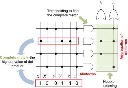
The simple logical structure shown in Fig. 1 acts very similar to the conventional ANNs. In fact, such a structure can be considered as a two-layer network. The first part of this structure, which consists of input and hidden layers (i.e., the layer consists of AND gates) is used to create the min-terms and the second part, which consists of hidden and output layers (i.e., the layer consists of OR gates) is used to add the products and generate the final outputs. It is well-known that any binary function can be constructed by using such a three-layer network. Clearly, similar to conventional ANNs [20], in the structure shown in Fig. 1 increasing the number of layers will not enhance the accuracy of the resulted binary function.

In order to gain more insight about the similarities between ANNs and logical circuits, we can describe the role of the first two layers of the circuit shown in Fig. 1 in another manner. As it can be observed, each input of this circuit is multiplied in a specific weight, which is equal to either 1 or 0, and then it is entered to the hidden layer. Denote the weight matrix multiplied to the variables of input layer to form the variables of hidden layer as $\mathbf{W}_{1}^{\mathrm{logic}}$. Clearly, each row of this matrix, which is stored on cross-points of the first crossbar, corresponds to a certain combination of input variables. More precisely, the rows of $\mathbf{W}_{1}^{\mathrm{logic}}$ determine the min-terms used to create the functions at the system output, which are independent from the definition of output functions. Since $n$ input variables can generate, in general, $2^{n}$ min-terms, number of the rows of $\mathbf{W}_{1}^{\mathrm{logic}}$ is always smaller than or equal to $2^{n}$. However, as a general observation, digital functions usually do not need all of these $2^{n}$ min-terms to be constructed.

According to the above discussions, it seems that when the circuit shown in Fig. 1 is subjected to a certain binary input string, internal product of input variables and the pattern stored at each row of the crossbar (which corresponds to a specific min-term) is performed to determine the similarity between these two binary strings. Then each AND gate acts somehow as a neuron with hard-thresholding activation function (in contrast to OR gates which are soft-thresholding operators): Only the output of the AND gate (neuron) located on the row with complete agreement with input variables is set to 1 and the output of other AND gates (neurons) is set to 0. Note that although each AND gate here acts as a thresholding operator, unlike the activating function of neurons in ANNs, its thresholding level is determined beforehand and cannot be changed in practice. For example, when we have two input variables and one 3-input AND gate, we should set one of its input terminals equal to logic 1 to make sure that the activation of other two inputs can pass the threshold of the gate. Here, it is worth to mention that by recognizing the AND gate (or equivalently the min-term) with activated output in Fig. 1 one can determine the activated inputs and consequently, specify the concepts and events occurred simultaneously. In other words, it can be said that the activation of each min-term indicates the simultaneous occurrence of certain concepts (represented by input terminals). As it will be shown later, this method of determining the simultaneous happening of different events is of essential importance in designing our proposed neuro-fuzzy computing system.

In the second part of the circuit shown in Fig. 1 the min-terms generated in the first part are combined together to produce the final outputs of the system. But, unlike the first part, the weights connecting the AND gates of hidden layer to the OR gates of output layer are not predictable and fully dependent on the definition of binary functions. However, interesting point is that these weights can be adjusted following the Hebbian learning rule [18] used in ANNs. More precisely, it can be easily verified that when for a certain input the output of system is equal to logic 1, output of the activated AND gate (neuron) is connected to the activated output. It means that by the simultaneous applying the input and output data to input and output layers respectively, and using the Hebbian learning rule, the connections of the second part of the logical circuit can be constructed automatically. In addition, note that similar to most of the ANNs, thresholding strength of output neurons (i.e. OR gates) is weaker than the thresholding strength of neurons of the hidden layer (i.e. AND gates).

Although multi-layer logical circuits act very similar to ANNs, they have considerable advantages that we are trying to use them in our proposed computing system. Firstly, in logical circuits all input and output signals, as well as the weights stored in cross-points, are non-negative in nature. Secondly and more importantly, unlike ANNs, any binary function can be realized by training only the weights stored in the second crossbar of the two-layer logical circuit shown in Fig. 1 without using any optimization methods (recall that the pattern stored in the first crossbar is independent of the special binary functions aimed to be constructed, and moreover, this pattern can be determined only by knowing the number of input variables). Thirdly, assuming that $m_{i}$ and $\vee$ stand for the $i$th min-term and the OR operator respectively, we have $m_{i}\vee m_{i}=m_{i}$. It yields that repeated min-terms (i.e. putting emphasis on the simultaneous occurrence of several concepts or inputs) in the definition of a binary function (which is expressed in the form of sum of products) has no effect on the input-output relation of the resulted structure. In other words, assuming that the weights stored in the second crossbar are adjusted by using the Hebbian learning method, subjecting the system to repeated input-output data will not change anything in the system. Clearly, it is an important capability that ANNs do not have. Fourthly, any binary function can be expressed in the form of sum of products. This provides us with an easy way to explain and understand the role of binary functions based on the concepts occurring simultaneously since it is similar to the logic used by the brain of humankind. In other words, one can easily discover the task of a binary function expressed in the form of sum of products, while it is quite difficult to get such a knowledge by decoding the synaptic weights of the given ANN.

Finally, it should be noted that although using the complement of a binary variable provides us with no more information, it is still a common practice to use both a binary variable and its complement in logical circuit design. In fact, it seems that in the logical circuit design any distinct value of the input variable is considered as an individual or independent concept, which is probably because of the fact that our brain prefers to work with two contradicting concepts than a non-contradicting one. This is completely in contrast with ANNs in which we usually use only one input for each continuous input variable. In other words, similar to fuzzy logic [10], here it seems that we are considering one input terminal per each distinct value of input variable and the input that we apply to any of these terminals somehow is the representative of our confidence degree about the occurrence of its corresponding concept. For this reason, in the following discussions one input terminal is considered for each distinct value the input or output variable can take.

II-B The relation between logical circuits and fuzzy logic

One main question that arises at this point is: “Can we extend the multi-layer logical circuit shown in Fig. 1 such that it can work with non-binary input variables?”. Fortunately, the answer of this question is positive thanks to the fuzzy logic. In fact, the method used to express a binary function in the form of sum of products is very similar to the method of constructing a continuous function based on fuzzy rules. In the following we discuss on this subject with more details.

First, consider a multi-input-single-output fuzzy inference system whose input-output relation can be considered as the mathematical map $\mathbf{X}\rightarrow Y$, where $\mathbf{X}\subset\mathbb{R}^{n}$ and $Y\subset\mathbb{R}$. Moreover, assume that the output of this fuzzy inference system is obtained by aggregation of the output of $N$ fuzzy rules in the form of [21]:

$$R^{(k)}:\mathrm{IF}~{}x_{1}~{}\mathrm{is}~{}A_{1}^{k}~{}\mathrm{AND}~{}x_{2}~{}\mathrm{is}~{}A_{2}^{k}~{}\mathrm{AND}~{}\ldots~{}x_{n}~{}\mathrm{is}~{}A_{n}^{k}~{}$$

$$\qquad\qquad\mathrm{THEN}~{}y~{}\mathrm{is}~{}B^{k},\quad k=1,\ldots,N,$$ (1)

which, for better explanation of the similarities between fuzzy logic and logical circuits, can be rewritten as:

$$R^{(k)}:\mathrm{IF}~{}\mathbf{x}~{}\mathrm{is}~{}\mathbf{\Sigma}_{n}^{k}~{}\mathrm{THEN}~{}y~{}\mathrm{is}~{}B^{k}.$$ (2)

where $x_{i}$ ($i=1,2,\ldots,n$) and $y$ are input and output variables, respectively, $\mathbf{x}=[x_{1},x_{2},\ldots,x_{n}]\in\mathbf{X}$, $y\in Y$, $\{A_{1}^{k},A_{2}^{k},\ldots,A_{n}^{k}\}$ are fuzzy sets with membership functions $\mu_{A_{i}^{k}}(x_{i})$ ($i=1,2,\ldots,n$; $k=1,2,\ldots,N$) defined on the universal set of input variables, $B^{k}$ ($k=1,2,\ldots,N$) are fuzzy sets defined on the universal set of the output variable, and $\mathbf{\Sigma}_{n}^{k}$ is a n-dimensional fuzzy set with the following multi-input membership function:

$$\mu_{\mathbf{\Sigma}_{n}^{k}}(x_{1},x_{2},\ldots,x_{n})=t\left(\mu_{A_{1}^{k}}(x_{1}),\mu_{A_{2}^{k}}(x_{2}),\ldots,\mu_{A_{n}^{k}}(x_{n})\right),$$ (3)

where $t$ is a $t$-norm operator. Since the fuzzy propositions in the antecedent part of (II-B) are combined using the fuzzy AND operator, we call such rules AND-type fuzzy rules. According to the properties of the $t$-norm operator, the fuzzy proposition in the consequent part of an AND-type fuzzy rule is true (in fuzzy sense) if all of the fuzzy propositions in the antecedent part of that rule are true (again in fuzzy sense). Similarly, combination of the fuzzy propositions of the antecedent part with fuzzy OR leads to an OR-type fuzzy rule. Similar to logical circuits, AND-type fuzzy rules are often preferred since our brains find them more reasonable. Here, we can see the structural and behavioral similarities between fuzzy logic and logical circuits. For example, antecedent part of (II-B) plays the role of the creation of min-terms in the first part of the circuit shown in Fig. 1 but with the difference that here $A^{k}_{i}$s are fuzzy numbers (note that in logical circuits $A^{k}_{i}$s were crisp numbers chosen from the set $\{0,1\}$). In addition, aggregation of the output of $N$ fuzzy rules by using a $s$-norm operator is similar to the function of the second part of the logical circuit shown in Fig. 1. Finally, note that in fuzzy logic all inputs, outputs and coefficients are non-negative as well.

Now, let us look at the working procedure of each fuzzy rule in another way. According to (2) and (3) we interpret the antecedent part of each fuzzy rule as a subspace of $\mathbb{R}^{n}$ (denoted as $\mathbf{\Sigma}_{n}^{k}$) with non-crisp (fuzzy) borders. In fact, $\mathbf{x}^{\ast}\in\mathbb{R}^{n}$ belongs to the region defined by antecedent part of (2) if $\mu_{\mathbf{\Sigma}_{n}^{k}}(\mathbf{x}^{\ast})$ is a big number (i.e., it is close to unity), and vice versa. More precisely, it can be said that any $\mathbf{x}^{\ast}\in\mathbb{R}^{n}$ belongs to the subspace $\mathbf{\Sigma}_{n}^{k}$ with the confidence degree of $\mu_{\mathbf{\Sigma}_{n}^{k}}(\mathbf{x}^{\ast})$ (for $k=1,2,\ldots,N$). Clearly, lying the point corresponds to a crisp input data in any of these subspaces indicates the simultaneous happening of certain fuzzy concepts defined by these subspaces (or equivalently, the corresponding $A^{k}_{n}$s). For this reason, we call the subspace specified by antecedent part of each fuzzy rule a fuzzy min-term (in the special case when $A_{i}^{k}$ is a fuzzy set with singleton membership function from the support set of $\{0,1\}$, each fuzzy min-term is reduced to a logical min-term denoted as a single point in the space of input variables). Considering the fact that each of the fuzzy sets used in antecedent part of fuzzy rules can have a different membership function and support set, infinite number of unique fuzzy min-terms can be defined on the $n$-dimensional space of input variables. But, fortunately, in most of the real-world applications the input data are accumulated in certain parts of the space of input variables, and consequently, it is sufficient to define the limited number of fuzzy min-terms such that they cover only those areas. In other words, although the number of fuzzy min-terms theoretically can be very large, commonly only a few number of these min-terms have a considerable influence on the system output. Hence, in order to construct a fuzzy inference system we need to identify only the most important fuzzy min-terms (or fuzzy rules).

Now consider the case in which the $k$th rule given in (II-B) is subjected to the following fuzzy input data:

$$q:~{}x_{1}~{}\mathrm{is}~{}A^{\prime}_{1}~{}\mathrm{AND}~{}x_{2}~{}\mathrm{is}~{}A^{\prime}_{2}~{}\mathrm{AND}~{}\ldots\mathrm{AND}~{}x_{n}~{}\mathrm{is}~{}A^{\prime}_{n},$$ (4)

which can equivalently be expressed as:

$$q:~{}\mathbf{x}~{}\mathrm{is}~{}\mathbf{\Sigma}_{n}^{\prime},$$ (5)

where $\{A_{1}^{\prime},A_{2}^{\prime},\ldots,A_{n}^{\prime}\}$ are fuzzy sets with membership functions $\mu_{A_{i}^{\prime}}(x_{i})$ ($i=1,2,\ldots,n$), and $\mathbf{\Sigma}_{n}^{\prime}$ is a fuzzy set with multi-variable membership function $\mu_{\mathbf{\Sigma}_{n}^{\prime}}(\mathbf{x})$. The input data given in (4) stimulates the antecedent part of each of the fuzzy rules given in (II-B) to a certain degree. Clearly, the amount of activation of each fuzzy rule determines the contribution of the consequent part of that rule in the final output. Various methods are available to determine the amount of activation of the antecedent part of a fuzzy rule for the given fuzzy input data [21]. However, in the following we want to deal with this issue from a different point of view.

Consider again the fuzzy input data given in (5) which specifies the subspace $\mathbf{\Sigma}_{n}^{\prime}$ with fuzzy borders. In general, this subspace overlaps with the subspace of each of the fuzzy min-terms, i.e. $\mathbf{\Sigma}_{n}^{k}$s, in the $n$-dimensional space to a certain degree. But, unlike the binary logic, $\mathbf{\Sigma}_{n}^{\prime}$ most likely does not completely overlap with any of the $\mathbf{\Sigma}_{n}^{k}$s ($k=1,\ldots,N$) and consequently, here it is reasonable to assume that various fuzzy min-terms are activated to different degrees when the system is subjected to this fuzzy input. More precisely, the degree of activation of the $k$th fuzzy rule is proportional to the amount of overlapping between subspaces $\mathbf{\Sigma}_{n}^{k}$ and $\mathbf{\Sigma}_{n}^{\prime}$. So, similar to the binary logic, the fuzzy inference system first evaluates the similarity between the fuzzy input data and fuzzy min-terms and then applies a kind of soft-thresholding function (i.e., the $s$-norm operator) to determine the contribution of the output corresponding to each fuzzy min-term in the final outcome.

Here, we tried to show some of the similarities between fuzzy logic and logical circuits. On the other hand, in previous section we demonstrated how the aggregation of logical min-terms can be performed by using Hebbian learning rule. Therefore, it seems that by inspiration from logical circuits, we can propose a simple method to create fuzzy rules automatically based on the available training data. However, the main importance of the proposed method relates to its ability to work with ANNs. In fact, in the rest of this paper we will show that our proposed method can be used to train large scale ANNs, which can be considered as a big step toward the emulation of the computing power of human brain. This is mostly because of the fact that, as we will show in the next section, ANNs can be considered as systems that work with fuzzy concepts.

II-C Interpretation of ANNs as fuzzy inference systems

The aim of this section is to provide an answer to the following questions from a new point of view: (1) How similar is the behavior of ANNs to fuzzy inference systems? (2) How can we effectively and optimally determine and implement the fuzzy min-terms and consequently, inference engine of a very large-scale system? By answering the former question we can show that fuzzy inference systems have biological support. In order to answer these questions and finally propose our method for hardware implementation of neuro-fuzzy computing systems first we describe the function of ANNs based on fuzzy concepts in a new and interesting manner.

Figure 2: Typical artificial neural network with one hidden layer. In these systems, connection weights are usually determined during the learning process by the use of optimization methods.

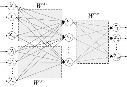
Consider the two-layer ANN shown in Fig. 2. In this figure:

• $\mathbf{x}=[x_{1},x_{2},\ldots,x_{nx}]$ and $\mathbf{y}=[y_{1},y_{2},\ldots,y_{ny}]$ are the vector of input variables entered to the input layer,

• $\mathbf{v}=[v_{1},v_{2},\ldots,v_{nv}]$, where $v_{i}$ is the output of neuron number $i$ of hidden layer,

• $\mathbf{W}^{xv}=[w_{ij}^{xv}]_{nv\times nx}$ is the matrix containing the weights connecting the neurons of input layer to the neurons of hidden layer, where $w_{ij}^{xv}$ is the weight of synapse connecting the $j$th entry of $\mathbf{x}$, $x_{j}$, to the $i$th entry of $\mathbf{v}$, $v_{i}$. Using this notation, output of neuron $i$ of the hidden layer, $v_{i}$, is obtained as:

  $$v_{i} = f\left(\sum_{l=1}^{nx}x_{l}w_{il}^{xv}+\sum_{l=1}^{ny}y_{l}w_{il}^{yv}\right)$$ (6)

  $$= f\left(\mathbf{w}_{i}^{xv}\mathbf{x}^{T}+\mathbf{w}_{i}^{yv}\mathbf{y}^{T}\right),~{}i=1,2,\ldots,nv,$$

  where $\mathbf{w}_{i}^{xv}=[w_{i1}^{xv},w_{i2}^{xv},\ldots,w_{inx}^{xv}]$, $\mathbf{w}_{i}^{yv}=[w_{i1}^{yv},w_{i2}^{yv},\ldots,w_{iny}^{yv}]$, and $f(.)$ is the activation function of the neurons of hidden layer.

• $\mathbf{W}^{vz}=[w_{ij}^{vz}]_{nz\times nv}$ is the matrix containing the weights connecting the neurons of hidden layer to the neurons of output layer, where $w_{ij}^{vz}$ is the weight of the synapse connecting the $j$th entry of $\mathbf{v}$, $v_{j}$, to the $i$th entry of $\mathbf{z}$, $z_{i}$.

• $z_{i}$ is the output of the $i$th neuron of output layer which can be expressed as follows:

  $$z_{i}=f\left(\sum_{l=1}^{nv}v_{l}w_{il}^{vz}\right)=f\left({\mathbf{w}}_{i}^{vz}\mathbf{v}^{T}\right),\quad i=1,2,\ldots,nz,$$ (7)

  where ${\mathbf{w}}_{i}^{vz}=[w_{i1}^{vz},w_{i2}^{vz},\ldots,w_{i,nv}^{vz}]$.

Figure 3 shows the realization of the ANN shown in Fig. 2. In this figure, matrices of synaptic weights are implemented by using the crossbar structure and it is assumed that the crossbars have the property that generate the sum of products of input variables in the weights stored at cross-points. For example, the signal entered to each neuron of hidden layer is equal to the sum of the product of signals at input layer to the synaptic weights stored at cross-points (i.e., the signal entered to the $i$th neuron of hidden layer is equal to $\mathbf{w}_{i}^{xv}\mathbf{x}^{T}+\mathbf{w}_{i}^{yv}\mathbf{y}^{T}$). In this figure typical values are assigned to synaptic weights and input data such that the height of each bar is proportional to the value of the corresponding variable or weight.

Figure 3: Simple realization of the ANN shown in Fig. 2 based on fuzzy concepts. In other words, this figure shows that it is possible to interpret the working procedure of conventional ANN similar to what we have in fuzzy inference system without changing its structure. In this figure, each row of the structure implements a simple fuzzy rule or min-term. In fact, here we have assumed that connection weight matrices model the universal sets of input and output variables and by programming their entries correctly, any fuzzy set can be created on these universal sets.

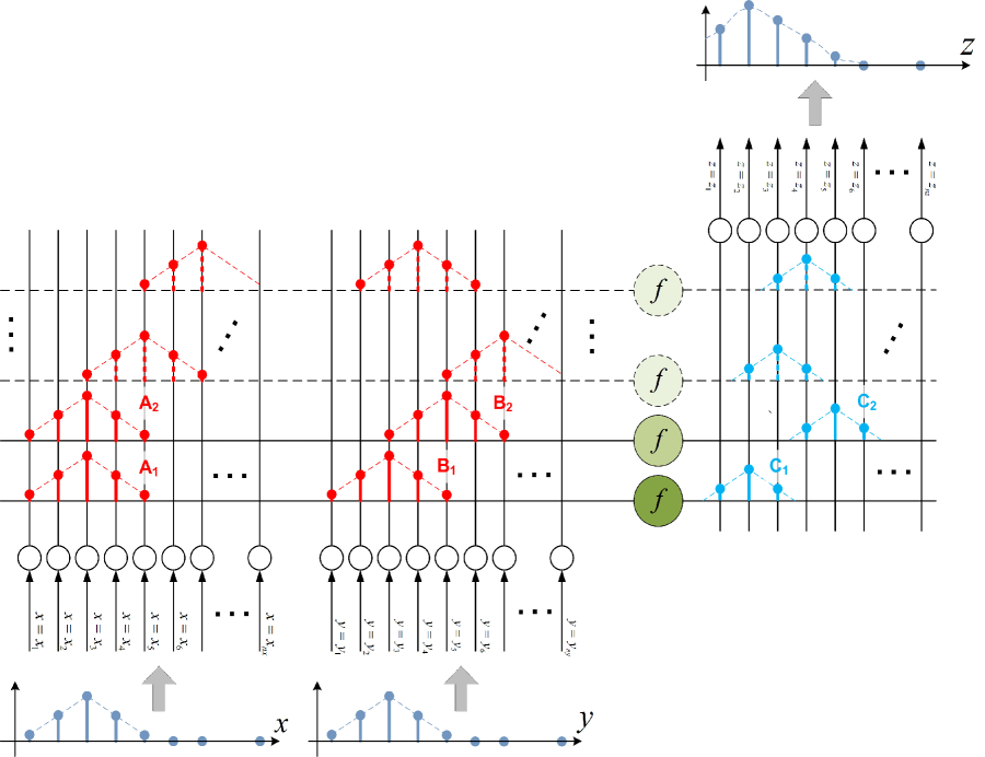
Interestingly, function of the structure shown in Fig. 2 can be interpreted in another way. In fact, similar to the case shown in Fig. 1, $x_{1},\ldots,x_{nx}$ and their corresponding vertical wires in the first crossbar can be considered as the representative of the different values or concepts the linguistic input variable $x$ can take. We have a similar situation for variables $y$ and $z$. In this case, at the input and output terminals and at the rows of the structure we have constructed the discrete universal set of the variables $x$, $y$ and $z$. Now, the special values assigned to $x_{1},\ldots,x_{nx}$ can be considered as the points of the membership function of the fuzzy input proposition “$x$ is $A^{\prime}$”. In other words, here it is assumed that the input applied to the $i$th input neuron shows our confidence degree about the occurrence of the concept assigned to that neuron for the observed fuzzy input data. Similarly, the synaptic weights stored at each row of the crossbar located between input and hidden (hidden and output) layer can be considered as the points of the membership function of the antecedent (consequent) part of the corresponding fuzzy rule. For example, Fig. 3 shows implementation of the fuzzy sets $A_{1}$ and $B_{1}$ (defined on the universal set of $x$ and $y$, respectively) based on the coefficients stored at the lowest row of the weight matrices $\mathbf{W}^{xv}$ and $\mathbf{W}^{yv}$, respectively. Clearly, in this structure any new fuzzy rule can be added to the fuzzy rule-base simply by adding a new row to the first structure and then adjusting the weights to appropriate values.

Now we can explain the function of the first part of the ANN shown in Fig. 3, which is mathematically described in (6). Since we assumed that all inputs and synaptic weights show the confidence degrees and consequently are non-negative variables, we can conclude that the dot-product of $\mathbf{x}$ and $\mathbf{w}_{i}^{xv}$ (as well as $\mathbf{y}$ and $\mathbf{w}_{i}^{yv}$) indicates the similarity between these two vectors (or the concepts represented by these membership functions). For example, it is obvious that larger the value of $\mathbf{w}_{i}^{xv}\mathbf{x}^{T}$ larger the similarity between $\mathbf{w}_{i}^{xv}$ and $\mathbf{x}$ and therefore larger our confidence degree about the occurrence of the predefined concept $\mathbf{w}_{i}^{xv}$ at the input variable $x$. This fact provides us with a new explanation for the task of the thresholding function in ANNs. To make it clear, consider again the equation relates the output of neurons of hidden layer to the inputs and synaptic weights:

$$v_{i}=f\left(\mathbf{w}_{i}^{xv}\mathbf{x}^{T}+\mathbf{w}_{i}^{yv}\mathbf{y}^{T}\right),\quad i=1,2,\ldots,nv.$$ (8)

In the above equation without using the thresholding function $f$ it is not possible to determine whether the output is caused by only one of the inputs or both of them. By suitable choice of this function the output of neuron $i$ is activated only when both $\mathbf{x}$ and $\mathbf{y}$ are similar to $\mathbf{w}_{i}^{xv}$ and $\mathbf{w}_{i}^{yv}$, respectively. Clearly, activation of the $i$th neuron of hidden layer indicates the simultaneous occurrence of the concepts defined by $\mathbf{w}_{i}^{xv}$ and $\mathbf{w}_{i}^{yv}$. Hence, the role of thresholding function $f$ in (8) is somehow similar to the role of AND gates in logical circuits. However, since here the probability of having a complete match is very low, hard-thresholding activation function cannot be used. It concludes that in Fig. 3 each row of the crossbar located between input and hidden layers implements the antecedent part of a fuzzy rule, and the output of corresponding neuron in hidden layer shows the amount of activation of that rule (fuzzy min-term) for the given input.

The task of the soft thresholding function, $f$, used in the neurons of hidden layer can also be interpreted in another way. In Section II-B we mentioned that the amount of activation of the $k$th fuzzy rule is proportional to the amount of overlap between subspaces $\mathbf{\Sigma}_{n}^{k}$ and $\mathbf{\Sigma}_{n}^{\prime}$. So, the question here is: How can we measure the amount of overlap between two $n$-dimensional subspaces by using the typical integrated circuits (which are actually two-dimensional devices)? A simple and efficient answer is that we can measure the similarity at each dimension separately and then combine the results (by using a $t$-norm type operator) to obtain the total similarity between $\mathbf{\Sigma}_{n}^{k}$ and $\mathbf{\Sigma}_{n}^{\prime}$. It concludes that the thresholding function, $f$, in ANNs plays the role of $t$-norm operator in fuzzy inference systems. For example, it can be observed that the ANN shown in Fig. 3 first measures the similarity at each dimension separately (by calculating $\mathbf{w}_{i}^{xv}\mathbf{x}^{T}$ and $\mathbf{w}_{i}^{yv}\mathbf{y}^{T}$ in $x$ and $y$ dimensions, respectively) and then applies the thresholding function to the sum of these two values to detect the simultaneous occurrence of predefined concepts (i.e. $\mathbf{w}_{i}^{xv}$ and $\mathbf{w}_{i}^{yv}$). As mentioned before, a good method to combine the similarities obtained at each dimension separately is to use an operator that acts somehow as the fuzzy $t$-norm operator. More precisely, if $a$ and $b$ are two variables of confidence-degree type (which indicate the similarity between input variables and the antecedent part of fuzzy rules stored at the rows of crossbar) the operator $T$ that combines them should have the property:

$$\mathrm{if}~{}a\leq b~{}\mathrm{then}~{}T(a,b)\leq a.$$ (9)

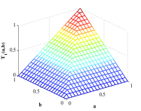
But, assuming $a=\mathbf{w}_{i}^{xv}\mathbf{x}^{T}$ and $b=\mathbf{w}_{i}^{yv}\mathbf{y}^{T}$ the thresholding function given in (8) leads to $T(a,b)=f(a+b)$ which, in general, does not satisfy (9). However, by suitable choice of $f$ it can be observed that this function acts very similar to the fuzzy $t$-norm operator or the p-input logical AND gate. For example in Fig. 4 we have compared the results obtained by applying four different operators defined as: $T_{1}(a,b)=\min(a,b)$, $T_{2}(a,b)=(a+b)^{3}$, $T_{3}(a,b)=(a+b)^{9}$, and $T_{4}(a,b)=\mathrm{tansig}((a+b)-3)=2/\left(1+\exp\left(-2*(a+b-3)\right)\right)-1$ to the operands $a$ and $b$ such that $0\leq a,b\leq 1$. Note that in this figure output of each operator is normalized such that it lies between 0 and 1. As it can be seen in this figure, operators $T_{2}$ and $T_{4}$ (which is a very common activation function in ANNs) acts similar to fuzzy $t$-norm operator $T_{1}$. In addition, Fig. 4(c) shows that by increasing the power in the definition of operator $T_{2}$ this operator can be reduced to the 2-input logical AND gate.

(a) $T_{1}(a,b)=min(a,b)$

(b) $T_{2}(a,b)=(a+b)^{3}$

(c) $T_{3}(a,b)=(a+b)^{9}$

(d) $T_{4}(a,b)=tansig((a+b)-3)$

Figure 4: Comparison between different operators. This figure verifies that the proposed activation function, i.e. $(a+b)^{p}$, acts similar to other $t$-norm operators. In addition, by comparing the shape of operators $T_{2}$ and $T_{4}$ it can be said that the activation function of neurons in ANNs to some extend is a $t$-norm operator.

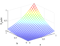
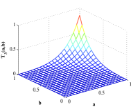
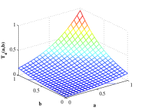
Now, we can study that part of circuit located between hidden and output layers. In this part of circuit, the weight matrix $\mathbf{W}^{vz}$ is implemented by using the crossbar structure similar to previous discussions. It is also assumed that the value of each neuron at output layer indicates the confidence degree to a certain point in the universal set of output variable (or the concept represented by that output neuron). Hence, the values generated by neurons of output layer constitute the membership function of output fuzzy number. Note that the output of the ANN shown in Fig. 3 can still be connected to the input of another ANN of this type. The weight matrix $\mathbf{W}^{vz}$ determines which output and to what extent should be activated when a fuzzy min-term is activated (or equivalently, when certain concepts occurred simultaneously at the input). Note that in this structure we have actually assumed that the learning is the procedure of making appropriate connections between fuzzy min-terms and output concepts (but not between input and output fuzzy concepts). It concludes that the elements of the weight matrix $\mathbf{W}^{vz}$ can easily be adjusted by applying the Hebbian learning method (as described in Section II-A) to the neurons of output and hidden layer. It means that when for a certain input-output data a neuron in output layer is activated simultaneous to a neuron in hidden layer, the synaptic weight connecting these two neurons should be amplified and the amount of this amplification should be proportional to the strength of activation of the corresponding two neurons. Interestingly, in [10] we showed that this process is also equivalent with the creation of fuzzy relation [21] between min-terms and output concepts. Note that the membership function of the consequent part of each fuzzy rule is constructed on a row of the second crossbar and the final fuzzy output is equal to the weighted sum (aggregation) of these membership functions, where the weight assigned to each membership function is proportional to the strength of activation of the antecedent part of that fuzzy rule.

The interpretation proposed in this section for the function of ANNs has many advantages to the classical descriptions. First, in this method all input data, output data and synaptic weights are non-negative. Second, unlike other training methods (such as back-propagation) in the proposed structure the appropriate value of synaptic weights can be obtained without the need to optimization methods. The main reason for this statement is that the first crossbar of the ANN shown in Fig. 3 implements the fuzzy min-terms which can be constructed independent of the definition of final input-output relation.

To sum up, in this section we showed that the operation of ANNs can be interpreted in a quite different way without applying any changes to the classical structure. Moreover, we showed that the two-layer ANN can be considered as a fuzzy inference system with fuzzy input and fuzzy output. In the next section we present a method of hardware implementation and training the proposed neuro-fuzzy computing system, which is obtained by inspiration from logical circuits, fuzzy logic and ANNs. We will also show that the proposed neuro-fuzzy system is really effective and can be used to solve some of the complicated engineering problems.

III Realization, training and application of the proposed neuro-fuzzy system

In this section we explain the hardware implementation, training and some applications of our proposed nuero-fuzzy system, which has considerable differences with existing methods. It will also be shown that the proposed structure has the advantage that can effectively be designed to deal with massive input-output data.

The overall structure of the proposed neuro-fuzzy computing system is the same as the one depicted in Fig. 3, which can also be considered as a two-layer network. In this figure, without any loss of generality, it is assumed that $x$ and $y$ are scalar inputs and $z$ is the scalar output. Note that this system is actually a dynamical structure which is incomplete at the beginning and being more and more completed by training it with the new data. It means that the hidden layer does not have any neurons before training and the neurons are generated right after subjecting the system to input-output training data. For this purpose, first the neurons of input layer should be divided to few groups such that the number of groups be equal to the number of input variables. The number of neurons at each group is, in general, different with others and depends on the accuracy required to model the variable corresponds to that group. In fact, at each group one neuron is required for any new concept or value that input variable can take. For example, 101 neurons are required to deal with a variable that varies between 0 and 10 with the resolution of 0.1. In this case, the first neuron will represent concept “$x=0$”, the second neuron will represent concept “$x=0.1$” and so on. Clearly, by increasing the number of neurons at input layer any input variable can be constructed with a desired accuracy. Similarly, one neuron should be considered at output layer for any distinct value of the output signal. For the given input, the signal generated at each neuron of output layer shows the confidence degree of system to the special value or concept assigned to that neuron. Hence, the output of this system is actually a fuzzy data which can be converted to a crisp number by applying any defuzzification method.

It is assumed that the output of each neuron at input layer is exactly equal to its input (i.e., it has identity activation function), and the output of each neuron at output layer is equal to the weighted sum of the signals entered to it (again having identity activation function). As it can be observed in Fig. 3 for each of the input variables a fuzzy set with any desired membership function can be constructed on each row of the crossbar located between input and hidden layers. For example, in this figure the fuzzy sets $A_{1}$ and $A_{2}$ are constructed on the universal set of $x$ and the fuzzy sets $B_{1}$ and $B_{2}$ are constructed on the universal set of $y$. It will be shown later that the fuzzy sets constructed on the rows of this crossbar constitute the antecedent part of if-then type fuzzy training data.

III-A Response of the proposed neuro-fuzzy computing system to the given input

In this section we assume that the proposed neuro-fuzzy computing system is designed and fully trained, and we discuss only on different aspects of computing its output for the given input. The training procedure will then be discussed in Section III-B. Note that, as it will be shown later, the proposed system can be trained during its ordinary work and the only reason for presenting the training procedure in another section is for the sake of clarity.

In Fig. 3 assume that $x^{\ast}_{i}$ is the value of the signal entered to the $i$th neuron of the group corresponding to variable $x$, $x_{i}$ is the concept assigned to the $i$th neuron of this group, $y^{\ast}_{i}$ is the value of the signal entered to the $i$th neuron of the group corresponding to variable $y$, $y_{i}$ is the concept assigned to the $i$th neuron of this group, $nx$ is the number of neurons used to cover the universal set of the fuzzy variable $x$, $ny$ is the number of neurons used to cover the universal set of the fuzzy variable $y$, $z^{\ast}_{i}$ is the value observed at the $i$th neuron of output layer, $z_{i}$ is the concept assigned to the $i$th neuron of output layer, $nz$ is the number of neurons used to cover the universal set of the fuzzy variable $z$, $v_{i}$ is the output of $i$th neuron of hidden layer, $N_{v}^{k}$ is the number of neurons at hidden layer after applying $k$ set of input-output training data, $\mathbf{W}^{xv}=\left\{w_{ij}^{xv}\right\}_{N_{v}^{k}\times nx}$ is the weight matrix containing the coefficients connecting the neurons corresponding to variable $x$ in input layer to the neurons of hidden layer, $\mathbf{W}^{yv}=\left\{w_{ij}^{yv}\right\}_{N_{v}^{k}\times ny}$ is the weight matrix containing the coefficients connecting the neurons corresponding to variable $y$ in input layer to the neurons of hidden layer, and $\mathbf{W}^{vz}=\left\{w_{ij}^{vz}\right\}_{nz\times N_{v}^{k}}$ is the weight matrix containing the coefficients connecting the neurons of hidden layer to the neurons of output layer. Using these notations if we denote the input vectors as $\mathbf{x}^{\ast}=[x^{\ast}_{1},x^{\ast}_{2},\ldots,x^{\ast}_{nx}]$ and $\mathbf{y}^{\ast}=[y^{\ast}_{1},y^{\ast}_{2},\ldots,y^{\ast}_{ny}]$, output of the $i$th neuron at hidden layer is obtained as

$$v_{i}=f\left(\mathbf{w}_{i}^{xv}{\mathbf{x}^{\ast}}^{T}+\mathbf{w}_{i}^{yv}{\mathbf{y}^{\ast}}^{T}\right) = \left(\mathbf{w}_{i}^{xv}{\mathbf{x}^{\ast}}^{T}+\mathbf{w}_{i}^{yv}{\mathbf{y}^{\ast}}^{T}\right)^{p},$$

$$i = 1,2,\ldots,N_{v}^{k},~{}~{}p>1,$$ (10)

where $f(.)$ is the activation function of neurons, $\mathbf{w}_{i}^{xv}$ is the $i$th row of $\mathbf{W}^{xv}$ and $\mathbf{w}_{i}^{yv}$ is the $i$th row of $\mathbf{W}^{yv}$. The main difference between (III-A) and similar equations observed in classical ANNs is in the activation function, which is considered as $f(s)=s^{p}$ here. In the following we will discuss on the reason of using this type of activation function in more details.

Consider again the neuro-fuzzy system shown in Fig. 3. As mentioned before, each row of the first crossbar contains the membership function of two fuzzy sets, and each fuzzy set is constructed by equating the synaptic weight stored at each cross-point to the value of the corresponding membership function at that point. According to the previous discussions, the data stored at each row of the first crossbar constitutes a fuzzy min-term, which approximately refers to a unique combination of two fuzzy input variables. It concludes that in practice each distinct input-output training data can form the antecedent part of an AND-type fuzzy rule, which is stored on one row of the first crossbar. For example, the second row of the first crossbar in Fig. 3 implements the antecedent part of the following fuzzy rule:

$$\mathrm{IF}~{}x~{}\mathrm{is}~{}A_{2}~{}\mathrm{AND}~{}y~{}\mathrm{is}~{}B_{2}~{}\mathrm{THEN}~{}z~{}\mathrm{is}~{}C_{2}.$$ (11)

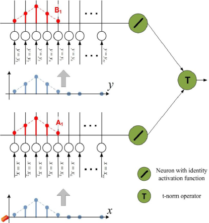
In order to evaluate the output of each neuron at hidden layer for the given fuzzy inputs first the similarity between the membership function of each fuzzy input and the corresponding pattern (membership function) stored at each row of the crossbar is determined by calculating the internal product of these two membership functions. For example, in the second row of crossbar this procedure is equivalent to the calculation of $\mathbf{w}_{2}^{xv}{\mathbf{x}^{\ast}}^{T}$ for variable $x$ and $\mathbf{w}_{2}^{yv}{\mathbf{y}^{\ast}}^{T}$ for variable $y$. Now, in order to determine the output of the $i$th neuron of hidden layer, which shows the amount of activation of the corresponding fuzzy rule, the values obtained for $\mathbf{w}_{2}^{xv}{\mathbf{x}^{\ast}}^{T}$ and $\mathbf{w}_{2}^{xv}{\mathbf{y}^{\ast}}^{T}$ should be combined using a $t$-norm type operator. In fact, the operator that combines $\mathbf{w}_{2}^{xv}{\mathbf{x}^{\ast}}^{T}$ and $\mathbf{w}_{2}^{yv}{\mathbf{y}^{\ast}}^{T}$ should have the property that generates considerably big outputs only when both of these two numbers are considerably large. One possible approach for hardware implementation of such a $t$-norm is to use the structure shown in Fig. 5. The main drawback of this structure, as well as the logical circuit shown in Fig. 1, is that the number of inputs of the $t$-norm operator depends on the number of fuzzy inputs of system. Note that in order to simulate the behavior of brain we need to develop structures with numerous number of inputs and outputs where each output is the function of only a few but different number of inputs. But, if in the structure shown in Fig. 3 we use different $t$-norm operators with different number of inputs, the resulted hardware will be very complicated and inefficient. Equation (III-A) proposes that the $t$-norm of $\mathbf{w}_{i}^{xv}{\mathbf{x}^{\ast}}^{T}$ and $\mathbf{w}_{i}^{yv}{\mathbf{y}^{\ast}}^{T}$ be defined as $\left(\mathbf{w}_{i}^{xv}{\mathbf{x}^{\ast}}^{T}+\mathbf{w}_{i}^{yv}{\mathbf{y}^{\ast}}^{T}\right)^{p}$, where $p>1$ is an arbitrary integer. As explained before and showed in Fig. 4, it can be easily verified that for the values of $p>>1$ the output of each neuron, when both $\mathbf{w}_{i}^{xv}{\mathbf{x}^{\ast}}^{T}$ and $\mathbf{w}_{i}^{yv}{\mathbf{y}^{\ast}}^{T}$ are large, is much bigger than the case when either $\mathbf{w}_{i}^{xv}{\mathbf{x}^{\ast}}^{T}$ or $\mathbf{w}_{i}^{yv}{\mathbf{y}^{\ast}}^{T}$ is large. Although the activation function defined in (III-A) does not satisfy all requirements of a $t$-norm operator, we will show in Section V that it works very well in practice. Moreover, it has the advantage that unlike other activation functions used in classical ANNs does not have any thresholding or other parameters to tune. Another advantage of this activation function is that it leads to a structure whose hidden layer is not changed by increasing the number of the system inputs.

Figure 5: This figure shows how the activation function of neurons can be implemented when the activation function is modeled by a $t$-norm operator. This implementation has this drawback that it depends completely on the number of input variables.

Considering the output of hidden layer as $\mathbf{v}=[v_{1},v_{2},\ldots,v_{N_{v}^{k}}]$, output of the $i$th neuron at output layer in Fig. 3 is obtained as

$$z^{\ast}_{i}={\mathbf{w}}_{i}^{vz}\mathbf{v}^{T},\quad i=1,2,\ldots,nz,$$ (12)

where ${\mathbf{w}}_{i}^{vz}=[w_{i1}^{vz},w_{i2}^{vz},\ldots,w_{i,N_{v}^{k}}^{vz}]$ is the $i$th row of $\mathbf{W}^{vz}$. Equation (12) can be expressed in vector form as

$$\mathbf{z}^{\ast}=[z^{\ast}_{1},z^{\ast}_{2},\ldots,z^{\ast}_{nz}]=\mathbf{v}\left(\mathbf{W}^{vz}\right)^{T}.$$ (13)

where the dimension of $\mathbf{W}^{vz}$ is $nz\times N_{v}^{k}$.

As it can be observed, this part of system acts very similar to the second layer of classical ANNs and the only difference is that the activation function of neurons at the output layer of Fig. 3 is of identical type. In fact, the output vector $\mathbf{z}^{\ast}$ determines the membership function of the resulted fuzzy output for the given fuzzy inputs.

III-B Training the proposed neuro-fuzzy computing system

In the previous section we showed that the working procedure of all parts of the proposed neuro-fuzzy computing system, except the activation function of neurons at hidden layer, are similar to a classical ANN. However, what makes the proposed system considerably different and efficient is the procedure of its training. More precisely, the proposed system is trained using supervisory method based on the given input-output data, and as it will be shown later, training the synaptic weights or other parameters of the system can be performed without the need to any optimization method. Without any loss of generality, consider again the neuro-fuzzy computing system shown in Fig. 3 and assume that the system already has been subjected to $k$ input-output training data and currently it has $N_{v}^{k}\leq k$ neurons at hidden layer. In the following we discuss on the method of training the system when it is subjected to a new training data.

Assume that we are given the $(k+1)$th input-output training data and our goal is to train the system such that it learns this new data. Note that since the system under consideration has two inputs and one output, the new training data must consist of two fuzzy sets as input variables and a fuzzy set as output variable. But, in the following, for the sake of simplicity we will assume that the input training data consists of two fuzzy sets while the output training data is a crisp number. Denote the fuzzy training inputs as $\mathbf{x}^{\ast}$ and $\mathbf{y}^{\ast}$, and apply them to the corresponding neurons of input layer (recall that each set of neurons at input layer covers the universal set of the corresponding fuzzy input). According to the previous discussions, applying these fuzzy inputs to system will cause the activation of the output of each neuron at hidden layer to a certain degree. Then the output of neurons of hidden layer are combined together according to (13) to form the membership function of the output variable. Defuzzifying this fuzzy output leads to a crisp number as the final output. If the difference between this number and the output training data be less than a predefined threshold we can conclude that the system already has been trained with a very similar training data and consequently we do not need to train the system with this new data again. Two points should be noted here. First, since we assumed that the output training data is a crisp number we have to defuzzify the output of our neuro-fuzzy computing system in order to be able to compare it with the training data. However, in some applications the output training data is itself a fuzzy concept (hereafter denoted as $\mathbf{u}^{\ast}$) and consequently no defuzzification is required at the output layer. In this case the difference between the output training data and output of the neuro-fuzzy computing system can be measured by calculating, e.g., the internal product of these two output vectors (membership functions of the two fuzzy numbers). Second, the value of this threshold can easily be determined according to the accuracy needed by user and without the need to any optimization. Obviously, decreasing the value of this parameter will increase the accuracy of system at the cost of using more fuzzy min-terms (or equivalently, more neurons at hidden layer).

When the difference between the output generated by the neuro-fuzzy computing system and the given training output is larger than the predefined threshold value the system should be trained with the new training data. In fact, the main reason causes the system not to be able to generate an accurate output for the given input data is that it has not been subjected to a similar data before. In this case first we create a new fuzzy min-term by adding a new neuron to hidden layer and then we apply appropriate changes to the synaptic weights stored in the second crossbar to make the final output closer to the output training data.

The simplest way to create a new fuzzy min-term (to cover the subspace specified by this new data) is to store the membership functions of the new input data at the cross-points connecting the neurons of input layer to the new neuron added to hidden layer. For this purpose we can simply store $\mathbf{x}^{\ast}$ and $\mathbf{y}^{\ast}$ (which are the membership functions describing input data) at the new row added to the first crossbar. Hence, after adding the neuron number $N_{v}^{k}+1$ to the hidden layer of system we set

$$\mathbf{w}_{N^{k}_{v}+1}^{xv}=\mathbf{x^{\ast}},$$ (14)

and

$$\mathbf{w}_{N^{k}_{v}+1}^{yv}=\mathbf{y^{\ast}}.$$ (15)

In this case, the output of this newly added hidden neuron will become active only when the applied input data is close enough to the trained data characterized by $\mathbf{x}^{\ast}$ and $\mathbf{y}^{\ast}$. Now, in order to apply appropriate changes to the synaptic weights stored in the second crossbar (to form connections between min-terms and output concepts) first we calculate the output of neurons of hidden layer as

$$v_{i}=f\left(\mathbf{w}_{i}^{xv}{\mathbf{x}^{\ast}}^{T}+\mathbf{w}_{i}^{yv}{\mathbf{y}^{\ast}}^{T}\right)=\left(\mathbf{w}_{i}^{xv}{\mathbf{x}^{\ast}}^{T}+\mathbf{w}_{i}^{yv}{\mathbf{y}^{\ast}}^{T}\right)^{p},$$

$$\quad\quad\quad i=1,2,\ldots,N_{v}^{k}+1,~{}~{}p>1.$$ (16)

Then we update the synaptic weights stored in the weight matrix $\mathbf{W}^{vz}$ using the Hebbian learning method. In this method the weight of the synapse connecting two active neurons (one in hidden and another in output layer) is amplified proportional to the amount of activation of these two neurons. More precisely, after calculating the output of neurons at hidden layer, the synaptic weight connecting the $i$th neuron of hidden layer to the $j$th neuron of output layer is updated as follows:

$$w_{ij}^{vz}\leftarrow w_{ij}^{vz}+\alpha t(v_{j},u_{i}),\quad i=1,\ldots,nz,~{}j=1,\ldots,N_{v}^{k}+1,$$ (17)

where $u_{i}$ is the value of the output training data, i.e. $\mathbf{u}^{\ast}$ at the $i$th output neuron, $\alpha$ is the learning coefficient, and $t$ is the t-norm operator used to implement the Hebbian learning method. Note that since the latest fuzzy min-term added to the neuro-fuzzy computing system is exactly the same as the membership function of fuzzy inputs, output of the $(k+1)$th neuron of hidden layer would be much bigger than the output of other neurons at this layer when the system is subjected to the latest inputs, $\mathbf{x^{\ast}}$ and $\mathbf{y^{\ast}}$. Hence, according to (17) the synaptic weights connecting the $(N_{v}^{k}+1)$th neuron of hidden layer to the neurons of output layer (i.e., the coefficients on the $(N_{v}^{k}+1)$th row of $\mathbf{W}^{vz}$) are mainly affected by the Hebbian learning method. By repeating the above procedure for any new input-output training data, the structure becomes more and more completed. Interesting point in relation to the training of this system is that, unlike many other training methods, each input-output data is applied only once and consequently problems like over-training never occur. Moreover, according to (17) this system can be trained by using both fuzzy and crisp data without the need to any optimization algorithm.

It may seem that the proposed neuro-fuzzy computing system just stores the input-output training data and does not perform any computation. But, by taking into account the possible overlaps between fuzzy min-terms, it is observed that the size of the data stored in system can be much smaller than the size of the input-output training data, specially in dealing with long-term records. In most of the practical cases the rate of adding new min-terms to the system is (almost monotonically) decreased by carrying on the training procedure. Finally, note that another advantage of the proposed neuro-fuzzy computing system is that memory and computing units are assimilated together, which is similar to what has happened in all of the living things.

IV Hardware implementation of the proposed neuro-fuzzy computing system

In this section, we will discuss on advantages of the proposed computing system from the hardware implementation point of view. During the explanation of the proposed method in previous sections the reader may have recognized that the suggested learning algorithm is not perfect and can be easily improved in different ways (e.g., by modifying membership functions of the programmed fuzzy sets). However, in the following we will show that the main reason for suggesting this special structure is its simple hardware implementation. For this purpose first remember that our main goal is to design a computing system with the ability of emulating the computing power of human brain. Therefore, by considering the structural complexity and size of the real neuron, simplicity of the hardware is of critical importance for its success. This means that the final system should be easily expandable by merging basic computing units and it should have a simple content- or concept-based learning method (similar to content-based addressable memories with computing ability) which can be easily mapped into hardware. Hence, using any kind of optimization method is not allowed evidently since their hardware implementation is very costly and inefficient even for a small network.

Now let us see how the proposed system can be implemented in practice. As stated in Section III-A, during the ordinary work of system, both parts of the structure shown in Fig. 3 perform simple vector to matrix multiplication (see Eqs. (III-A) and 13). Note that in this case, the $t$-norm operator or the activation function of neurons is applied to the results obtained from these vector to matrix multiplications. Figure 6 shows the proposed circuit to perform vector to matrix multiplication. This circuit consists of a simple memristor crossbar [22] where each of its rows is connected to the virtually grounded terminal of an operational amplifier that plays the role of a neuron with identity activation function. The memristor crossbar structure has two sets of conductive parallel wires crossing each other perpendicularly such that at each crosspoint a semiconductor device is fabricated between two crossing wires. In the structure shown in Fig. 6 this semiconductor element is a memristive device [4, 23]. Memristive device is a nonlinear element whose resistance (known as memristance) can be tuned by applying a suitable voltage to the device [24]. Since there is a threshold in the physical model of the device, amplitude of the applied voltage should be larger than this threshold to be able to change the state (and consequently, the memristance) of the device [25]. Hence, assuming that the amplitude of the voltages applied to the circuit of Fig. 6 is below the threshold of memristive devices, output of the $i$th neuron (operational amplifier), $O_{i}$, can be written as:

$$O_{i}=-\sum_{j=1}^{n}\left(\frac{R_{f}}{M_{ij}}\right)I_{j}=-\sum_{j=1}^{n}R_{f}G_{ij}I_{j}$$ (18)

Figure 6: Memristor crossbar-based circuit proposed to do vector to matrix multiplication which can be used for the hardware implementation of the proposed neuro-fuzzy system.

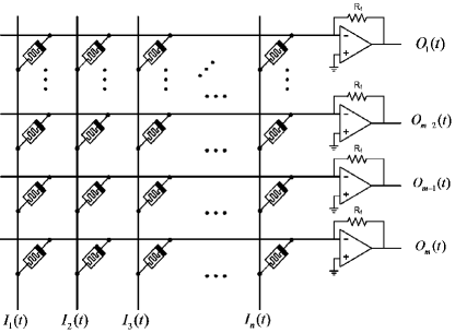
where $M_{ij}$ and $G_{ij}$ are the memristance and memductance (inverse of memristance) of the memristive device located in the crossing point of the $i$th row and the $j$th column of the crossbar, $R_{f}$ is the feedback resistor of operational amplifiers and $I_{j}$ is the input voltage applied to the $j$th column of the crossbar. Note that since the memristance of memristive devices is not changing during this computation, in Eq. (18) they have been treated as ordinary resistors. By comparing Eqs. (18) and (III-A) (or Eqs. (18) and (13)) it becomes clear that this structure is a perfect circuit to implement the proposed method. For this purpose, connection weight matrices (which contain the membership function of corresponding fuzzy sets) should be stored as a memductance of memristive devices in crosspoints of the crossbar. On the other hand, each neuron should compute the weighted sum of its inputs and then apply the activation function to the result. This can be done by applying a suitable non-linear function, e.g. $f(\cdot)=(\cdot)^{p}$, to the output of operational amplifiers in Fig. 6. Finally, it is evident that the computing structure shown in Fig. 3 can be implemented by series connection of two of these memristor crossbar structures (i.e., connecting the outputs of one of these circuits directly to the inputs of another one).

Now, consider the learning process described in Section III-B. As explained in that section, the learning process of the proposed method consists of two different phases: (i) creation of min-terms (storing fuzzy sets) on the first crossbar (which connect the neurons of input layer to the neurons of hidden layer) and (ii) updating the connection weights stored in crosspoints of the second crossbar (which connect the neurons of hidden layer to the neurons of output layer). In order to add a new min-term to the sample of the structure shown in Fig. 6, first a new row should be added to the first crossbar of this structure. For this purpose from the beginning we can reserve some of the rows of the first crossbar for storing upcoming data. In this case adding a new row is equivalent to tuning the memristance of the memristors located on an unused row to suitable values. In order to store weights on the newly added row (or equivalently, storing the membership function of fuzzy input sets) we interpret the value of the membership function at each point as a voltage signal and then we apply it to the corresponding column of the crossbar. Now, by grounding the new row while other rows are connected to a high impedance, current will pass through the memristors connected to this row. Assuming that all of these memristors initially have a same memristance and considering the fact that the amount of electrical current passing through a memristor is proportional to the amplitude of the voltage applied to it, it can be concluded that the conductance of each memristor on the newly added row is proportional to the amplitude of the voltage applied to the corresponding column (or equivalently, to the membership function of fuzzy input at that column). This means that only by applying membership functions to columns of the first crossbar while newly added row is grounded and then waiting for specific time, a new min-term corresponding to the input training data automatically will be added to the crossbar. Note that several methods have been proposed so far to change the memristance of specified memristors in a crossbar without altering the memristance of other semi-selected memristors [22].

Now, let us consider the problem of hardware implementation of the second phase of the proposed learning method on the structure shown in Fig. 6, which is used to implement the second crossbar in Fig. 3 (from hidden layer to output layer). In fact, here we want to update the corresponding weights (i.e. memductance of memristors) based on the given training data. It is concluded from Eq. (17) that for any given training data, memductance (connection weight) of the memristor connecting a neuron of hidden layer to a neuron of output layer should be changed such that the amount of this change be proportional to the sum of the firing strength of these two neurons. In order to implement this updating method in the memristive structure shown in Fig. 6, first we inject the input training data to system and let the neurons of hidden layer generate their own output signals (see Eq. (III-A)). Then, we interpret the value of membership function of the output fuzzy training data (or $\mathbf{u^{\ast}}$) at any point as a voltage signal and apply the negative of this voltage to its corresponding column of the crossbar. In this case, the current passing through the memristor connecting a hidden neuron to an output neuron will be proportional to the voltage dropped across this memristor, which is equal to the sum of the absolute value of the voltages applied to row and column of the crossbar that this memristor is located between them. For example, for the memristor located in the crossing point of the $i$th row and the $j$th column of the crossbar this voltage will be equal to $u_{i}+v_{j}$. Now, application of this voltage will cause the memristance(memductance) of the memristor to decrease(increase) which will increase the weight $w_{ij}=\frac{R_{f}}{M_{ij}(t)}$ stored in this memristor (so the relation expressed in Eq. (17)). Figure 7 shows how the weight stored in a typical memristor, i.e. $w_{ij}=\frac{R_{f}}{M_{ij}(t)}$, changes versus the amplitude of the voltage $u_{i}+v_{j}$ when it is applied to the device for a specific period of time. In this figure, $R_{f}$ and the initial memristance of the memristor are considered equal to $R_{off}$ (the maximum memristance that the memristor can have).

Figure 7: This figure shows how the weight stored in the memristor typically changes versus the applied voltage during the learning process. From this figure it can be figured out that a single memristor acts as a $t$-norm operator. It changes the stored value (memristance of the memristor) significantly when the voltage across the device is big (so the probability that both voltages at terminals of memristor have big values is high as well). In this simulation the HP model [4] is used to simulate memristor and voltages are applied to memristor for about 0.05 second.

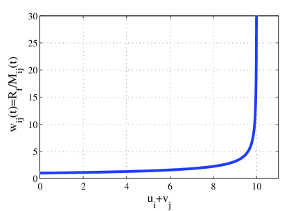
By comparing Figs. 7 and 4 it can be inferred that each memristor somehow applies a $t$-norm operator to the two voltages connected to its terminals (so the function $t(u_{i},v_{j})$ in Eq. (17)): when both voltages have high values (i.e. the neurons are fired simultaneously), the weight stored in the memristor is increased much more than the case in which only one of these neurons is fired. This means that at the end of this learning procedure, we will see a strong connection only between those hidden and output neurons that usually fire simultaneously. To summarize, to carry out this learning process we should only apply training data to input and output terminals of the structure and wait some period of time. This will cause the memristance of memristors to change based on the Hebbian learning rule similar to what we had in Eq. (17). To conclude, by using two of these memristor crossbar structures, connecting them to each other correctly and managing the amplitude and timing of the applied voltages corresponding to training data, the proposed neuro-fuzzy system or any rule-based fuzzy inference method can be simply constructed.

V Simulation results

In this section we show the high potential of the proposed neuro-fuzzy computing system for solving different engineering problems in the field of modeling and classification. One important capability of the proposed system is to model multi-variable mathematical functions. To show this, consider the functions:

$$g_{1}(x,y)=10.391((x-0.4)(y-0.6)+0.36),$$ (19)

$$g_{2}(x,y)=24.234\left(r^{2}(0.75-r^{2})\right),\ \ r^{2}=(x-0.5)^{2}+(y-0.5)^{2},$$ (20)

$$g_{3}(x,y) = 42.659\left(0.1+\widetilde{x}\left(0.05+\widetilde{x}^{4}-10\widetilde{x}^{2}\widetilde{y}^{2}+5\widetilde{y}^{4}\right)\right),$$ (21)

$$\widetilde{x}=x-0.5,\quad\widetilde{y}=y-0.5,$$

$$g_{4}(x,y) = 1.3356\left(1.5(1-x)+e^{2x-1}\sin(3\pi(x-0.6)^{2})\right)$$ (22)

$$+ 1.3356\left(e^{3(y-0.5)}\sin(4\pi(y-0.9)^{2})\right),$$

$$g_{5}(x,y)=1.9(1.35+e^{x}\sin(13(x-0.6)^{2})e^{-y}\sin(7y)),$$ (23)

which are proposed by Hwang et al. [26] to study the learning and modeling capability of systems (in all of the above functions it is assumed that $x,y\in[0,1]$). In the following we use the structure shown in Fig. 3 to model each of these functions, which are also shown in Fig. 8.

(a) $g_{1}$

(b) $g_{2}$

(c) $g_{3}$

(d) $g_{4}$

(e) $g_{5}$

Figure 8: Graph of functions $g_{1}$ to $g_{5}$.

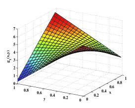
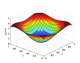
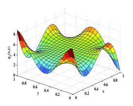
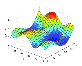
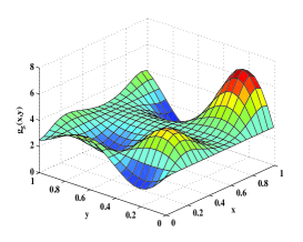
In each simulation the neuro-fuzzy computing system is subjected to 225 training data and 10,000 test data, which are randomly selected from the space of input variables. Moreover, power of the activation function of neurons at hidden layer (i.e., the value of $p$ in (III-A)) and the value of $\alpha$ in (17) are considered equal to 7 and 0.0005, respectively (these values are obtained by a simple trial and error and it is observed during numerical simulations that the final results are not so sensitive to the values assigned to these parameters). The Fraction of Variance Unexplained (FVU) performance index defined as follows [26]

$$FVU=\frac{\sum_{i=1}^{10000}(g(x_{i},y_{i})-\widehat{g}(x_{i},y_{i}))^{2}}{\sum_{i=1}^{10000}(g(x_{i},y_{i})-\overline{g})^{2}},$$

$$\quad\overline{g}=\frac{1}{10000}\sum_{i=1}^{10000}g(x_{i},y_{i}),$$ (24)

is used to evaluate the modeling accuracy of the resulted neuro-fuzzy computing systems, where $g(x_{i},y_{i})$ and $\widehat{g}(x_{i},y_{i})$ are the values generated by function itself and the proposed neuro-fuzzy computing system, respectively. Table I summarizes the simulation results. Note that since the original training data consist of crisp numbers, in all simulations each input data is subjected to a fuzzification as shown in Fig. 9 before entering to the system. In this fuzzification process, the support set of the resulted fuzzy number should be chosen proportional to the number of available training data and the accuracy required for modeling the function. By increasing of the number of training data, smaller support set can be chosen to reach higher modeling accuracy. Table I shows that, for example, 100 neurons are used to cover the universal set of $x$ and $y$, and 116 neurons are used to cover the universal set of $z$, when modeling of $g_{1}$ is aimed. According to the domain of definition and the range of $g_{1}$ it concludes that the variables $x$, $y$, and $z$ are modeled with the maximum accuracy of 0.01, 0.01, and 0.06, respectively.

TABLE I: Accuracies of the models optimized using the proposed method.

Function	# of neurons for variable $x$	# of neurons for variable $y$	# of neurons for variable $z$	Threshold value	$FVU$	# of constructed min-terms
$g_{1}$	100	100	116	0.2	0.067	77
$g_{2}$	100	100	69	0.1	0.044	161
$g_{3}$	100	100	143	0.1	0.263	140
$g_{4}$	100	100	105	0.2	0.087	123
$g_{5}$	100	100	126	0.15	0.09	130

Figure 9: Fuzzification process used to convert crisp training data to their corresponding fuzzy numbers.

Table II summarizes the results obtained by modeling $g_{1}$,…,$g_{5}$ with other methods. The first group of the results presented in this table corresponds to the modeling of these functions by the ANNs trained using back-propagation and Projection Pursuit Learning (PPL) method (under different conditions and structures). The second group of the results presented in Table II corresponds to the method proposed by Kwok and Yeung [27] for training the coefficients of the new hidden units added to a dynamical network based on using different cost functions (i.e., $S_{1}$, $\sqrt{S_{1}}$, $S_{2}$, $\sqrt{S_{2}}$, $S_{3}$, $\sqrt{S_{3}}$, $S_{cascor}$, $S_{fujita}$, and $S_{sqr}$ as defined in [27]). The third group of results in Table II is obtained by using the method proposed by Ma and Khorasani [28], which is similar to the previous method with the difference that instead of using different cost functions for training, different Hermite polynomial activation functions are applied to the neurons of hidden layer. Murakami and Honda [29] studied the modeling ability of the Active Learning Method (ALM) and used it for pattern-based information processing. The ALM divides the input space into several partitions and then models the function in each of these partitions through a simple pattern. Finally, the last group of results in Table II corresponds to the modeling of functions using the ANFIS method [30].

TABLE II: Comparing the accuracies of the models optimized using different algorithms based on FVU criterion [29].

Ref.	Model	Function
		$g_{1}$	$g_{2}$	$g_{3}$	$g_{4}$	$g_{5}$
[26]	BPL based on Gauss-Newton method (5 hidden units)	0.001	0.065	0.506	0.080	0.142
	BPL based on Gauss-Newton method (10 hidden units)	0.001	0.002	0.183	0.003	0.021
	PPL supersmoother (3 hidden units)	0.000	0.010	0.355	0.021	0.135
	PPL supersmoother (5 hidden units)	0.000	0.007	0.248	0.000	0.028
	PPL Hermite (3 hidden units)	0.000	0.009	0.075	0.001	0.049
	PPL Hermite (5 hidden units)	0.000	0.000	0.000	0.001	0.015
[27]	CFNN with $S_{1}$	0.021	0.029	0.269	0.036	0.121
	CFNN with $\sqrt{S_{1}}$	0.011	0.028	0.247	0.037	0.111
	CFNN with $S_{2}$	0.095	0.426	0.547	0.636	0.610
	CFNN with $\sqrt{S_{2}}$	0.024	0.031	0.275	0.031	0.134
	CFNN with $S_{3}$	0.003	0.020	0.306	0.027	0.160
	CFNN with $\sqrt{S_{3}}$	0.003	0.018	0.288	0.030	0.167
	CFNN with $S_{cascor}$	0.025	0.027	0.265	0.031	0.121
	CFNN with $S_{fujita}$	0.004	0.047	0.444	0.070	0.246
	CFNN with $S_{sqr}$	0.007	0.038	0.573	0.185	0.294
[28]	Standard CFNN with sigmoidal activation functions (10 hidden units)	0.048	0.097	0.551	0.073	0.206
	Proposed CFNN with Hermite polynomial activation functions (10 hidden units)	0.031	0.027	0.197	0.076	0.095
	Standard CFNN with sigmoidal activation functions (20 hidden units)	0.043	0.048	0.303	0.050	0.111
	Proposed CFNN with Hermite polynomial activation functions (20 hidden units)	0.026	0.019	0.082	0.027	0.039
[29]	ALM with 6 partitions	0.014	0.031	0.153	0.057	0.076
	ALM with 7 partitions	0.015	0.027	0.132	0.060	0.062
	ALM with 8 partitions	0.021	0.032	0.129	0.061	0.063
	ALM with 9 partitions	0.027	0.035	0.122	0.067	0.064
[30]	ANFIS with 9 rules	0.000	0.002	0.033	0.008	0.089

Comparing the modeling errors of $g_{1}$ in Tables I and II leads to the fact that the proposed neuro-fuzzy computing system is less effective than other methods for the modeling of approximately linear functions such as $g_{1}$. The main reason for this problem is that the proposed system divides the space of input variables into several overlapping subspaces (min-terms) and tries to model the given function in each of these subspaces by a single IF-THEN rule. However, it is a well-known fact that by the aggregation of this kind of rules (which has a simple fuzzy set in their consequent part), it is very difficult to model a linear function. It is also concluded from Table I that in all cases a high percent of training data is stored in the crossbar. The reason for this problem is that since the number of training data is not large enough, most of the input-output training pairs contain a new information and tend to constitute a new fuzzy min-term. It will be shown later that this problem can be removed simply by increasing the number of input-output training pairs.

Here, it is worth to emphasize on three important notes. Firstly, although some other neuro-fuzzy systems such as ANFIS can outperform the proposed system, but they have the disadvantage that after their training the resulted fuzzy sets and rules conceptually have almost no meaning. Secondly, except the ALM, all other methods are relied on optimization methods, which means that they do not have biological support and they cannot be implemented in large scale. In addition, they suffer from the very high computational cost. Finally, it should be noted that unlike almost all other methods, in the proposed computing system each training data is presented to the system only once.

Table III shows the effect of increasing the number of training data on the accuracy and the number of constructed fuzzy min-terms of the resulted system. Note that in each case the number of fuzzy min-terms is equal to the number of dissimilar training data sufficient to construct the system. It is concluded from Table III that the proposed neuro-fuzzy system can effectively model the functions under consideration by considering only some of the most important fuzzy min-terms (training data). Another observation is that the accuracy of system can considerably be increased by increasing the number of input-output training data. Finally, note that since in all simulations parameters of the proposed neuro-fuzzy computing system are obtained by trial and error (and consequently, are not optimal), it is expected that better results can be achieved by using optimally selected parameters.

TABLE III: Accuracies of the models optimized using the proposed method with different numbers of training data.

Function	$g_{1}$		$g_{3}$		$g_{5}$
# of training data	400	700	400	700	400	700
FVU	0.026	0.021	0.153	0.117	0.058	0.036
# of min-terms	194	238	216	245	189	229

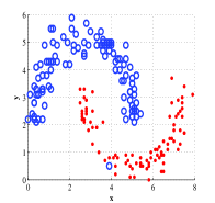
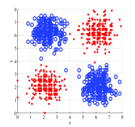
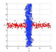
In the following we discuss on the ability of the proposed neuro-fuzzy system for data classification. The reason for the importance of this problem is that it shows the ability of system for making suitable decisions in facing with new environmental inputs. For this purpose consider four different data sets (each consists of two different objects) as shown in Fig. 10. In each case first we train the system shown in Fig. 3 with only two output terminals (one per each class) using supervisory method. Then we present the new data points to system and let it classify them. Table IV shows the details of the parameters used in simulations and the results obtained at each case. Figure 11 shows an example of how the new data points have been classified by the trained system. It is also concluded from Table IV that in all cases only a small fraction of the whole training data is sufficient to construct a neuro-fuzzy computing system with the ability of data classification with a high precision.

TABLE IV: Classification rate (%) for each test set

Data set	# of neurons for variable $x$	# of neurons for variable $y$	# of training data	# constructed minterms	classification rate (%)
1	100	100	335	52	99.8
2	90	90	200	45	99.36
3	98	98	1000	107	99.64
4	94	94	600	40	95.83

(a) Data set #1

(b) Data set #2

(c) Data set #3

(d) Data set #4

Figure 10: Data sets used to demonstrate the ability of the proposed neuro-fuzzy system for data classification.

(a) Data set #1

(b) Data set #2

(c) Data set #3

(d) Data set #4

Figure 11: This figure shows an example of how the new data points have been classified by the trained system.

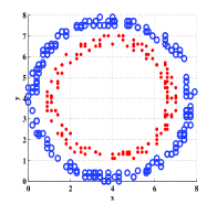
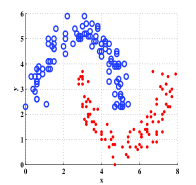
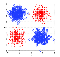
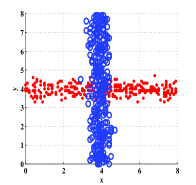
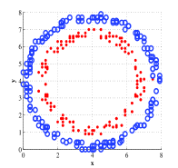
Finally, we can study the performance of the proposed neuro-fuzzy computing system when it is trained with the noisy data or when a certain percent of the memristors at cross-points are distorted randomly. First consider the problem of modeling $g_{1}$,…,$g_{5}$ (as defined in (19)-(23)) when the system is trained with the noisy data. For this purpose, we add a Gaussian noise with zero average and variance of 0.01 to each of the 225 input-output training data, and then we train the system shown in Fig. 3 using these noisy data (recall that the original data are randomly selected (with uniform distribution) from the domain of definition of the corresponding functions). Table V shows the values obtained for FVU under the above-mentioned conditions in a typical simulation. These results show the good robustness of the proposed system in dealing with noisy data. Repeating the above simulation assuming that the training data is not noisy but 20 percent of the cross-points are randomly distorted beforehand and cannot be used to save data, we arrive at the results presented in Table VI (a randomly chosen value is assigned to each distorted memristor during simulation). These results clearly show that the proposed system can fairly tolerate such a distortion. In fact, in this case the number of fuzzy min-terms is automatically increased to improve the accuracy of system.

TABLE V: Noise tolerance of models using FVU criterion

Function	$g_{1}$	$g_{2}$	$g_{3}$	$g_{4}$	$g_{5}$
FVU	0.281	0.394	0.727	0.586	0.61

TABLE VI: Fault tolerance of the proposed structure in modeling application using FVU criterion

Function	$g_{1}$	$g_{2}$	$g_{3}$	$g_{4}$	$g_{5}$
FVU	0.212	0.096	0.357	0.144	0.228
# of constructed min-terms	96	186	156	152	139

VI Conclusion

One novelty of this paper is in the new explanation presented for the relation between logical circuits and ANNs, logical circuits and fuzzy logic, and ANNs and fuzzy inference systems. This explanation led to the notion of fuzzy min-terms and a special two-layer ANN with the capacity of working with fuzzy input-output data. This neuro-fuzzy computing system has at least four main advantages compared to many other classical designs. First, it can effectively be realized on the nano-scale memristor-crossbar structure. Second, the hardware of system can be trained simply by applying the Hebbian learning method and without the need to any optimization. Third, the proposed structure can effectively work with huge number of input-output training data (of fuzzy type) without facing with problems like overtraining. Finally, it has a strong biological support, which makes it a powerful structure to emulate the function of human brain.

References

- [1] N. M. Botros and M. Abdul-Aziz, “Hardware implementation of an artificial neural network using field programmable gate arrays (FPGA’s),” IEEE Transactions on Industrial Electronics, Vol. 41, No. 6, pp. 665–667, December 1994.
- [2] A. Dinu, M. N. Cristea, and S.E. Cristea, “Direct Neural-Network Hardware-Implementation Algorithm,” IEEE Transactions on Industrial Electronics, Vol. 57, No. 5, pp. 1845–1848, May 2010.
- [3] Y. H. Kuo, C. I. Kao, and J. J. Chen, “A fuzzy neural network model and its hardware implementation,” IEEE Transactions on Fuzzy Systems, Vol. 1, No. 3, pp. 171–183, 1993.
- [4] D.B. Strukov, G.S. Snider, D.R. Stewart and R.S. Williams, “The missing memristor found,” Nature, Vol. 453, pp. 80–83, 1 May 2008.
- [5] L.O. Chua, “Memristor - the missing circuit element,” IEEE Trans. on Circuit Theory, Vol. CT-18, No. 5, pp. 507–519, 1971.
- [6] G. Snider, R. Amerson, D. Carter, H. Abdalla, M.S. Qureshi, J. Léveillé, M. Versace, H. Ames, S. Patrick, B. Chandler, A. Gorchetchnikov, and E. Mingolla, “From synapses to circuitry: Using memristive memory to explore the electronic brain,” Computer, Vol. 44, No. 2, pp. 21–28, 2011.
- [7] S. H. Jo, T. Chang, I. Ebong, B. B. Bhadviya, P. Mazumder and W. Lu, “Nanoscale Memristor Device as Synapse in Neuromorphic Systems,” Nano Letter, Vol. 10, No. 4, pp. 1297–1301, March 2010.
- [8] T. Chang, S.-H. Jo, and W. Lu, “Short-Term Memory to Long-Term Memory Transition in a Nanoscale Memristor,” ACS Nano, Vol. 5, No. 9, pp. 7669–7676, 2011.
- [9] F. Merrikh-Bayat, S. Bagheri Shouraki, and A. Rohani, “Memristor Crossbar-Based Hardware Implementation of the IDS Method,” IEEE Transactions on Fuzzy Systems, Vol. 19, No. 6, pp. 1083–1096, December 2011.
- [10] F. Merrikh-Bayat, and S. Bagheri Shouraki, “Memristive Neuro-Fuzzy System,” To appear in IEEE Transactions on Systems, Man and Cybernetics, Part B: Cybernetics, 2012.
- [11] M. Versace, R. T. Kozma, and D. C. Wunsch, “Adaptive Resonance Theory Design in Mixed Memristive-Fuzzy Hardware,” Advances in Neuromorphic Memristor Science and Applications, Vol. 4, pp. 133–153, 2012.
- [12] W. Gerstner, R. Kempter, J. L. Hemmen and H. Wagner, “A neuronal learning rule for sub-millisecond temporal coding,” Nature, Vol. 383, pp. 76–78, 1996.
- [13] H. Kim, M. Sah, Y. Changju, T. Roska, and L.O. Chua, “Neural Synaptic Weighting With a Pulse-Based Memristor Circuit,” IEEE Transactions on Circuits and Systems I: Regular papers, Vol. 59, No. 1, pp. 148–158, 2012.
- [14] K.D. Cantley, A. Subramaniam, H.J. Stiegler, R.A. Chapman, and E.M. Vogel, “Hebbian Learning in Spiking Neural Networks With Nanocrystalline Silicon TFTs and Memristive Synapses,” IEEE Transactions on Nanotechnology, Vol. 10, No. 5, pp. 1066–1073, 2011.
- [15] A. Afifi, A. Ayatollahi, and F. Raissi, “Implementation of biologically plausible spiking neural network models on the memristor crossbar-based CMOS/nano circuits,” European Conference on circuit theory and design, pp. 563–566, 2009.
- [16] C. Zamarreño-Ramos, L. A. Camuñas-Mesa, J. A. Pérez-Carrasco, T. Masquelier, T. Serrano-Gotarredona, and B. Linares-Barranco, “On Spike-Timing-Dependent-Plasticity, Memristive Devices, and Building a Self-Learning Visual Cortex,” Frontiers in Neuroscience, Vol. 5, No. 26, 2011.
- [17] S. P. Adhikari, C. Yang, H. Kim, L.O. Chua, “Memristor Bridge Synapse-Based Neural Network and Its Learning,” IEEE Transactions on Neural Networks and Learning Systems, Vol. 23, No. 9, pp. 1426–1435, September 2012.
- [18] D. O. Hebb, “The organization of behavior,” New York Wiley and Sons, 1949.
- [19] V. P. Nelson, H. T. Nagle, B. D. Carroll, “Digital Logic Circuit Analysis and Design,” Prentice Hall, 1995.
- [20] L. V. Fausett, “Fundamentals of Neural Networks: Architectures, Algorithms and Applications,” Pearson Education Publisher, 2006.
- [21] L. Rutkowski, “Flexible Neuro-Fuzzy Systems: Structures, Learning and Performance Evaluation,” Kluwer Academic Publishers, 2004.
- [22] D.B. Strukov and K.K. Likharev, “Reconfigurable nano-crossbar architectures,” in: Nanoelectronics, R. Waser Eds., 2012.
- [23] L.O. Chua, and S. M. Kang, “Memristive devices and systems,” Proceedings of the IEEE, Vol. 64, No. 2, pp. 209–223, 1976.
- [24] F. Alibart, L. Gao, B. Hoskins, and D.B. Strukov, “High-precision tuning of state for memristive devices by adaptable variation-tolerant algorithm,” Nanotechnology 23, art. 075201, 2012.
- [25] E. Lehtonen, J. Poikonen, M. Laiho, W. Lu, “Time-dependency of the threshold voltage in memristive devices,” IEEE International Symposium on Circuits and Systems (ISCAS), pp. 2245–2248, 15-18 May 2011.
- [26] J. N. Hwang and S. R. Lay and M. Maechler and R.D. Martin and J. Schimert, “Regression modeling in back-propagation and projection pursuit learning,” IEEE Transactions on Neural Networks, Vol. 5, No. 3, pp. 342–353, 1994.
- [27] T. Y. Kwok and D. Y. Yeung, “Objective functions for training new hidden units in constructive neural networks,” IEEE Transactions on Neural Networks, Vol. 8, No. 5, pp. 1131–1148, 1997.
- [28] L. Ma and K. Khorasani, “Constructive feedforward neural networks using Hermite polynomial activation functions,” IEEE Transactions on Neural Networks, Vol. 16, No. 4, pp. 821–833, 2005.
- [29] M. Murakami and N. Honda, “A study on the modeling ability of the IDS method: A soft computing technique using pattern-based information processing,” International Journal of Approximate Reasoning, Vol. 45, pp. 470–487, 2007.
- [30] J. S. R. Jang, “ANFIS:Adaptive-Network-based Fuzzy Inference Systems,” IEEE Transactions on Systems, Man and Cybernetics, Vol. 23, pp. 665–685, 1993.