Convergence Theorems for the Non-Local Means Filter

Abstract

In this paper, we establish convergence theorems for the Non-Local Means Filter in removing the additive Gaussian noise. We employ the techniques of ”Oracle” estimation to determine the order of the widths of the similarity patches and search windows in the aforementioned filter. We propose a practical choice of these parameters which improve the restoration quality of the filter compared with the usual choice of parameters.

1 Introduction

We deal with the additive Gaussian noise model:

$$Y(x)=f(x)+\varepsilon(x),\;x\in\mathbf{I,}$$ (1)

where $\mathbf{I}$ is the uniform $N\times N$ grid of pixels on the unit square, $Y=\left(Y\left(x\right)\right)_{x\in\mathbf{I}}$ is the observed image brightness, $f:[0,1]^{2}\rightarrow\mathbf{R}_{+}$ is an original image (unknown target regression function) and $\varepsilon=\left(\varepsilon\left(x\right)\right)_{x\in\mathbf{I}}$ are independent and identically distributed (i.i.d.) Gaussian random variables with mean $0$ and standard deviation $\sigma>0.$

Important denoising techniques for the model (1) have been developed in recent years. A very significant step in these developments was the introduction of the Non-Local Means Filter by Buades et al buades2005review . For closely related works, see for example polzehl2006propagation ; kervrann2008local ; buades2009note ; Katkovnik2010local ; lou2010image .

The basic idea of the filters by weighted means is to estimate the unknown image $f(x_{0})$ by a weighted average of observations $Y(x)$ of the form

$$\widetilde{f}_{w}(x_{0})=\sum_{x\in\mathbf{U_{x_{0},h}}}w(x)Y(x),$$ (2)

where for each $x_{0}$ and $h>0$, $\mathbf{U}_{x_{0},h}$ denotes a square window with center $x_{0}$ and width $2h$, $w(x)$ are some non-negative weights satisfying $\sum_{x\in\mathbf{U}_{x_{0},h}}w(x)=1.$ The choice of the weights $w(x)$ is usually based on two criteria: a spatial criterion so that $w(x)$ is a decreasing function of the distance between $x$ and $x_{0}$, and a similarity criterion so that $w(x)$ is also a decreasing function of the brightness difference $|Y(x)-Y(x_{0})|$ (see e.g. yaroslavsky1985digital ; tomasi1998bilateral ), which measures the similarity between the pixels $x$ and $x_{0}$. In the Non-Local Means Filter, $h>0$ can be chosen relatively large, and the weights $w(x)$ are calculated according to the similarity between data patches $\mathbf{Y}_{x,\eta}=(Y(y):y\in\mathbf{U}_{x,\eta})$ (identified as a vector whose composants are ordered lexicographically) and $\mathbf{Y}_{x_{0},\eta}=(Y(y):y\in\mathbf{U}_{x_{0},\eta})$, instead of the similarity between just the pixels $x$ and $x_{0}$. Here $\eta>0$ is the size parameter of data patches.

The Non-Local Means Filter was further enhanced for speed in subsequent works by Mahmoudi and Sapiro (2005 (mahmoudi2005fast, )), Bilcu and Vehvilainen (2007 (bilcu2007fast, )), Karnati, Uliyar and Dey(2009 (karnati2009fast, )), and Vignesh, Oh and Kuo (2010 (vignesh2010fast, )). Other authors as Kervrann and Boulanger (2006 (kervrann2006optimal, ), 2008 (kervrann2008local, )), Chatterjee and Milanfar (2008 (chatterjee2008generalization, )), Buades, Coll and Morel (2006 (buades2006staircasing, )), Dabov, Foi, Katkovnik and Egiazarian (2007 (dabov2007image, ), 2009 (dabov2009bm3d, )) make the Non-Local method better. Thacker, Bromiley and Manjn (2008 (Thacker2008AQuantitative, )) investigate this basis in order to understand the conditions required for the use of Non-Local means, testing the theory on simulated data and MR images of the normal brain. Katkovnik, Foi, Egiazarian and Astola (2010 (Katkovnik2010local, )) review the evolution of the non-parametric regression modeling in imaging from the local Nadaraya-Watson kernel estimate to the Non-Local means and further to transform-domain faltering based on Non-Local block-matching.

Unfortunately, the ideal implementation of Non-Local Means is computationally expensive. Therefore, for the sake of rising the speed of denoising, only a neighborhood of the estimated point is considered. In practice, the similarity patches of size $7\times 7$ or $9\times 9$ and search windows of size $19\times 19$ or $21\times 21$ are often chosen. However these choices are empirical and the problem of optimal choice remains open. As a consequence, the results of the numerical simulations are not always satisfactory.

In this paper, we use the statistic estimation and optimization techniques to give a justification of the Non-Local Means filter, and to suggest the order of sizes of search window and similarity patch. Our main idea is to minimize a tight upper bound of the $L^{2}$ risk

$$R\left(\widetilde{f}_{w}(x_{0})\right)=\mathbb{E}\left(\widetilde{f}_{w}(x_{0})-f(x_{0})\right)^{2}$$

by changing the width of the search window. We first obtain an explicit formula for the optimal weights $w^{\ast}_{h}$ in terms of the unknown function $f.$ The corresponding weighted mean $f_{h}^{\ast}$ is called ”Oracle”; the ”Oracle” $f_{h}^{\ast}$ is shown to have an optimal rate of convergence and high performance in numerical simulations. To mimic the ”Oracle” $f_{h}^{\ast},$ we estimate $w_{h}^{\ast}$ by some adaptive weights $\widehat{w}_{h}$ based on the observed image $Y.$ We thus obtain the Non-Local Means Filter with the proper width of window. Numerical results show that the Non-Local Means Filter with proper width of window outperforms the Non-Local Means Filter with standard choice.

The paper is organized as follows. In Section 2, we introduce the ”Oracle” estimator of Non-Local Means Filter and reconstruct Non-Local Means Filter with the idea of ”Oracle” theory. Our main theoretical results are presented in Section 3 where we give the rate of convergence of the Non-Local Means Filter. In Section 4, we present our simulation results with a brief analysis. Section 5 gives the conclusion of our paper. Proofs of the main results are deferred to Section 6.

2 Main results

2.1 Notations

Let us set some notations to be used throughout the paper. The Euclidean norm of a vector $x=\left(x_{1},...,x_{d}\right)\in\mathbf{R}^{d}$ is denoted by $\left\|x\right\|_{2}=\left(\sum_{i=1}^{d}x_{i}^{2}\right)^{\frac{1}{2}}.$ The supremum norm of $x$ is denoted by $\|x\|_{\infty}=\sup_{1\leq i\leq d}\left|x_{i}\right|.$ The cardinality of a set $\mathbf{A}$ is denoted by $\text{card}\,\mathbf{A}$. For a positive integer $N$, the uniform $N\times N$ grid of pixels on the unit square is defined by

$$\mathbf{I}=\left\{\frac{1}{N},\frac{2}{N},\cdots,\frac{N-1}{N},1\right\}^{2}.$$ (3)

Each element $x$ of the grid $\mathbf{I}$ will be called pixel. The number of pixels is $n=N^{2}.$ For any pixel $x_{0}\in\mathbf{I}$ and a given $h>0,$ the square window of pixels

$$\mathbf{U}_{x_{0},h}=\left\{x\in\mathbf{I:\;}\|x-x_{0}\|_{\infty}\leq h\right\}$$ (4)

will be called search window at $x_{0}.$ We naturally take $h$ as a multiple of $\frac{1}{N}$ ($h=\frac{k}{N}$ for some $k\in\{1,2,\cdots,N\}$). The size of the square search window $\mathbf{U}_{x_{0},h}$ is the positive integer number

$$M=(2Nh+1)^{2}=\mathrm{card\ }\mathbf{U}_{x_{0},h}.$$ (5)

For any pixel $x\in\mathbf{U}_{x_{0},h}$ and a given $\eta>0$, a second square window of pixels $\mathbf{U}_{x,\eta}$ will be called patch at $x$. Like $h$, the parameter $\eta$ is also taken as a multiple of $\frac{1}{N}$. The size of the patch $\mathbf{U}_{x,\eta}$ is the positive integer

$$m=(2N\eta+1)^{2}=\mathrm{card\ }\mathbf{U}_{x_{0},\eta}.$$ (6)

The vector $\mathbf{Y}_{x,\eta}=\left(Y\left(y\right)\right)_{y\in\mathbf{U}_{x,\eta}}$ formed by the values of the observed noisy image $Y$ at pixels in the patch $\mathbf{U}_{x,\eta}$ will be called simply data patch at $x\in\mathbf{U}_{x_{0},h}.$

2.2 the ”Oracle” of Non-Local means

In order to study statistic estimation theory of the Non-Local Means algorithm, we introduce an ”Oracle” estimator (for details on this concept see Donoho and Johnstone (1994 (donoho1994ideal, ))) of Non-Local means. Denote

$$f^{\ast}_{h}=\sum_{x\in\mathbf{U}_{x_{0},h}}w^{\ast}_{h}Y(x),$$ (7)

where

$$w_{h}^{*}(x)=e^{-\frac{\rho_{f,x_{0}}^{2}(x)}{H^{2}}}\bigg{/}\sum_{y\in\mathbf{U}_{x_{0},h}}e^{-\frac{\rho_{f,x_{0}}^{2}(x)}{H^{2}}},\quad x\in\mathbf{U}_{x_{0},h},$$ (8)

$$\rho_{f,x_{0}}(x)\equiv|f(x)-f(x_{0})|$$ (9)

and $H>0$ is a constant. It is obvious that

$$\sum_{x\in\mathbf{U}_{x_{0},h}}w_{h}^{*}(x)=1\quad\text{and}\quad w_{h}^{*}(x)\geq 0.$$ (10)

Note that the function $\rho_{f,x_{0}}(x)\geq 0$ characterizes the similarity of the image brightness at the pixel $x$ with respect to the pixel $x_{0}$, therefore we shall call $\rho_{f,x_{0}}$ similarity function. The usual bias-variance decomposition of the Mean Squared Error (MSE)

$$\begin{split}&\mathbb{E}\left(f(x_{0})-f^{*}_{h}(x_{0})\right)^{2}\\ &=\left(\sum_{x\in\mathbf{U}_{x_{0},h}}w_{h}^{*}(x)\left(f(x)-f(x_{0})\right)\right)^{2}+\sigma^{2}\sum_{x\in\mathbf{U}_{x_{0},h}}w_{h}^{*}(x)^{2}\\ &\leq\left(\sum_{x\in\mathbf{U}_{x_{0},h}}w_{h}^{*}(x)\left|f(x)-f(x_{0})\right|\right)^{2}+\sigma^{2}\sum_{x\in\mathbf{U}_{x_{0},h}}w_{h}^{*}(x)^{2}\end{split}$$ (11)

The inequality (11) combining with (9) implies the following upper bound

$$\mathbb{E}\left(f(x_{0})-f^{*}_{h}(x_{0})\right)^{2}\leq g(w_{h}^{*}),$$ (12)

where

$$g(w)=\left(\sum_{x\in\mathbf{U}_{x_{0},h}}w(x)\rho_{f,x_{0}}(x)\right)^{2}+\sigma^{2}\sum_{x\in\mathbf{U}_{x_{0},h}}w(x)^{2}.$$ (13)

We shall define a family of estimates by minimizing the function $g\left(w^{*}_{h}\right)$ in $w^{*}_{h}$ and plugging the optimal weights into (7). We shall consider the local Hölder condition

$$|f(x)-f(y)|\leq L\|x-y\|_{\infty}^{\beta},\,\,\,\forall x,\,y\in\mathbf{U}_{x_{0},h+\eta},$$ (14)

where $\beta>0$ and $L>0$ are constants, $h>0$, $\eta>0$ and $x_{0}\in\mathbf{I}.$ The following theorem gives the rate of convergence of the ”Oracle” estimator and the proper width $h$ of the search window.

Theorem 2.1

Assume that $h=\left(\frac{\sigma^{2}}{4\beta L^{2}}\right)^{\frac{1}{2\beta+2}}n^{-\frac{1}{2\beta+2}}$ and $H>\sqrt{2}Lh^{\beta}$. Suppose that the function $f$ satisfies the local Hölder condition (14) and $f^{*}_{h}(x_{0})$ is given by (7). Then

$$\mathbb{E}\left(f^{*}_{h}(x_{0})-f(x_{0})\right)^{2}\leq\frac{2^{\frac{2\beta+6}{2\beta+2}}\sigma^{\frac{4\beta}{2\beta+2}}L^{\frac{4}{2\beta+2}}}{\beta^{\frac{2\beta}{2\beta+2}}}n^{-\frac{2\beta}{2\beta+2}}.$$ (15)

For the proof of this theorem see Section 6.1.

We confirm the theorem by simulations that the difference between the ”Oracle” $f_{h}^{\ast}(x_{0})$ and the true value $f(x_{0})$ is extremely small (see Table 1 and the definition of PSNR can be found in Section 4 ). The latter, at least from the practical point of view, the theorem justifies that it is reasonable to optimize the upper bound $g(w_{h}^{*})$ instead of optimizing the risk $\mathbb{E}\left(f_{h}^{\ast}(x_{0})-f(x_{0})\right)^{2}$ itself.

Theorem 2.1 displays that the choice of a small search window, in the place of the whole observed image, suffices to ensure a denoising without loss of visual quality, and explains why we take a small search window for the simulations in the Non-Local Means algorithm.

Table 1: PSNR values when ”Oracle” estimator $f_{h}^{\ast}$ is applied with different values of $M$.

Image	Lena	Barbara	Boats	House	Peppers
Size	$512\times 512$	$512\times 512$	$512\times 512$	$256\times 256$	$256\times 256$
$\sigma/PSNR$	10/28.12db	10/28.12db	10/28.12db	10/28.11db	10/28.11db
$9\times 9$	38.98db	37.26db	37.66db	38.93db	37.85db
$11\times 11$	40.12db	38.49db	38.80db	40.04db	38.85db
$13\times 13$	41.09db	39.55db	39.78db	40.98db	39.64db
$15\times 15$	41.92db	40.45db	40.63db	41.77db	40.39db
$17\times 17$	42.64db	41.23db	41.39db	42.40db	41.00db
$19\times 19$	43.29db	41.93db	42.06db	43.06db	41.58db
$21\times 21$	43.88db	42.57db	42.67db	43.61db	42.14db
$\sigma/PSNR$	20/22.11db	20/22.11db	20/22.11db	20/28.12db	20/28.12db
$9\times 9$	33.61db	31.91db	32.32db	33.72db	32.62db
$11\times 11$	34.78db	33.20db	33.49db	34.92db	33.65db
$13\times 13$	35.80db	34.28db	34.49db	35.98db	34.51db
$15\times 15$	36.69db	35.22db	35.40db	36.80db	35.26db
$17\times 17$	37.48db	36.05db	36.20db	37.48db	35.89db
$19\times 19$	38.17db	36.74db	36.90db	38.07db	36.45db
$21\times 21$	38.80db	37.40db	37.54db	38.67db	36.98db
$\sigma/PSNR$	20/22.11db	20/22.11db	20/22.11db	20/28.12db	20/28.12db
$9\times 9$	30.65db	28.89db	29.25db	30.69db	29.51db
$11\times 11$	31.83db	30.23db	30.45db	31.90db	30.51db
$13\times 13$	32.85db	31.33db	31.49db	32.92db	31.34db
$15\times 15$	33.74db	32.27db	32.37db	33.76db	32.08db
$17\times 17$	34.50db	33.09db	33.16db	34.48db	32.74db
$19\times 19$	35.20db	33.81db	33.85db	35.13db	33.32db
$21\times 21$	35.79db	34.46db	34.48db	35.71db	33.85db

2.3 Reconstruction of Non-Local Means filter

With the theory of ”Oracle” estimator, we reconstruct the Non-Local Means filter (buades2005review, ). Let $h>0$ and $\eta>0$ be fixed numbers. For any $x_{0}\in\mathbf{I}$ and any $x\in\mathbf{U}_{x_{0},h}$, the distance between the data patches $\mathbf{Y}_{x,\eta}=\left(Y\left(y\right)\right)_{y\in\mathbf{U}_{x,\eta}}$ and $\mathbf{Y}_{x_{0},\eta}=\left(Y\left(y\right)\right)_{y\in\mathbf{U}_{x_{0},\eta}}$ is defined by

$$d^{2}\left(\mathbf{Y}_{x,\eta},\mathbf{Y}_{x_{0},\eta}\right)=\left\|\mathbf{Y}_{x,\eta}-\mathbf{Y}_{x_{0},\eta}\right\|_{2}^{2},$$

where $\left\|\mathbf{Y}_{x,\eta}-\mathbf{Y}_{x_{0},\eta}\right\|_{2}^{2}=\frac{1}{m}\sum\limits_{y\in\mathbf{U}_{x,\eta}}$ $\left(Y(T_{x}y)-Y(y)\right)^{2}$, $T_{x}$ is the translation mapping: $T_{x}y=x+(y-x_{0})$ and $m$ is given by (6), which measures the similarity between the data patches $\mathbf{Y}_{x,\eta}$ and $\mathbf{Y}_{x_{0},\eta}$. Since $|f(x)-f(x_{0})|^{2}=\mathbb{E}|Y(x)-Y(x_{0})|^{2}-2\sigma^{2}$, an obvious estimator of $\mathbb{E}\left|Y(x)-Y(x_{0})\right|^{2}$ is given by $d^{2}\left(\mathbf{Y}_{x,\eta},\mathbf{Y}_{x_{0},\eta}\right)$. Define an estimated similarity function $\widehat{\rho}_{x_{0}}$ by

$$\widehat{\rho}_{x_{0}}^{2}(x)=d^{2}\left(\mathbf{Y}_{x,\eta},\mathbf{Y}_{x_{0},\eta}\right)-2\sigma^{2},$$ (16)

and an adaptive estimator $\widehat{f}_{h}$ by

$$\widehat{f}_{h}(x_{0})=\sum_{x\in\mathbf{U}_{x_{0},h}}\widehat{w}_{h}(x)Y(x),$$ (17)

where

$$\widehat{w}_{h} = e^{-\frac{\widehat{\rho}_{x_{0}}^{2}(x)}{H^{2}}}\bigg{/}\sum_{x^{\prime}\in\mathbf{U}_{x_{0},h}}e^{-\frac{\widehat{\rho}_{x_{0}}^{2}(x^{\prime})}{H^{2}}}$$ (18)

$$= e^{-\frac{d^{2}\left(\mathbf{Y}_{x,\eta},\mathbf{Y}_{x_{0},\eta}\right)}{H^{2}}}\bigg{/}\sum_{x^{\prime}\in\mathbf{U}_{x_{0},h}}e^{-\frac{d^{2}\left(\mathbf{Y}_{x^{\prime},\eta},\mathbf{Y}_{x_{0},\eta}\right)}{H^{2}}}.$$

and $\mathbf{U}_{x_{0},h}$ given by (4).

Note that $\Delta_{x_{0},x}(y)=|f(y)-f(T-xy)|$ and $\zeta(y)=\epsilon(T-xy)-\epsilon(y)$. It is easy to see that

$$\widehat{\rho}^{2}_{x_{0}}(x) = \frac{1}{m}\sum\limits_{y\in\mathbf{U}_{x_{0},\eta}}\left(f(x)+\epsilon(x)-f(x_{0})-\epsilon(x_{0})\right)^{2}-2\sigma^{2}$$

$$\leq \frac{1}{m}\sum\limits_{y\in\mathbf{U}_{x_{0},\eta}}\left(\Delta_{x_{0},x}(y)+\zeta(y)\right)^{2}-2\sigma^{2}$$

$$= \frac{1}{m}\sum\limits_{y\in\mathbf{U}_{x_{0},\eta}}\Delta^{2}_{x_{0},x}(y)$$

$$+\frac{1}{m}\sum\limits_{y\in\mathbf{U}_{x_{0},\eta}}\left(\zeta\left(y\right)^{2}-2\sigma^{2}+2\Delta_{x_{0},x}\left(y\right)\zeta\left(y\right)\right)$$

$$= \frac{1}{m}\sum\limits_{y\in\mathbf{U}_{x_{0},\eta}}\Delta^{2}_{x_{0},x}(y)+\frac{1}{m}S(x),$$

where

$$S(x)=\sum\limits_{y\in\mathbf{U}_{x_{0},\eta}}\left(\zeta\left(y\right)^{2}-2\sigma^{2}+2\Delta_{x_{0},x}\left(y\right)\zeta\left(y\right)\right).$$ (19)

Theorem 2.2

Assume that $\eta=c_{0}n^{-\alpha}$ $\left(\frac{(1-\beta)^{+}}{2\beta+2}<\alpha<\frac{1}{2}\right)$. Suppose that the function $f$ satisfies the local Hölder conditions (14) and $\widehat{\rho}_{x_{0}}$ is given by (25). Then there is a constant $c_{1}$ such that

$$\mathbb{P}\left(\max_{x\in\mathbf{U}_{x_{0},h}}\left|\widehat{\rho}_{x_{0}}^{2}(x)-\rho_{f,x_{0}}^{2}(x)\right|\geq c_{1}n^{\alpha-\frac{1}{2}}\sqrt{\ln n}\right)$$ (20)

$$= O\left(n^{-1}\right).$$

For the proof of this theorem see Section 6.2.

In the Theorem 2.2, we consider that $\sigma$ is a constant and the Hölder condition (14) implies that $\left|\frac{1}{\mathrm{card}\mathbf{U}^{\prime\prime}_{x_{0},\eta}}\right.$ $\left.\Delta_{x_{0},x}^{2}(y)-\rho_{f,x_{0}}^{2}(x)\right|=O\left(n^{\frac{2\beta}{2\beta+2}}\right)$. Therefore, if $n$ is large enough, we have $\left|\frac{1}{\mathrm{card}\mathbf{U}^{\prime\prime}_{x_{0},\eta}}\Delta_{x_{0},x}^{2}(y)-\rho_{f,x_{0}}^{2}(x)\right|\ll\sigma$. It is to say that the larger the standard deviation of the noise is, the more useful our theorem will be. We take the test image ”Lena” as an example, which is degraded by Gaussian noise with $\sigma=10$, $\sigma=20$ and $\sigma=30$ respectively. We fix the size of search window $M=13\times 13$, $H=0.4\times\sigma+2$ and choose the size of similarity patch $m\in\{2k+1:k=1,2,\cdots,20\}$. In the cases of $\sigma=20$ and $\sigma=30$, Figure 1 (b) and (c) illustrate that the value of PSNR value of increases when the size of a similarity patch increases. The evolutions of PSNR value are in accordance with Theorem 2.2. However, in the case of $\sigma=10$, Figure 1 (a) displays that the PSNR value increases when the size of a similarity patch increases in the interval $[3,15]$ and reaches the peak value. But it decreases in the interval $[15,41]$. This means that the value $\sigma=10$ is not large enough to satisfy the condition $\left|\frac{1}{\mathrm{card}\mathbf{U}^{\prime\prime}_{x_{0},\eta}}\Delta_{x_{0},x}^{2}(y)-\rho_{f,x_{0}}^{2}(x)\right|\ll\sigma$.

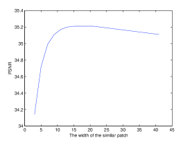
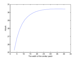
(a)$\sigma=10$	(b)$\sigma=20$	(c)$\sigma=30$

Figure 1: The evolution of PSNR value as a function of the size of a similarity patch.

In order to improve the results, we sometimes shall use the smoothed version of the estimate of brightness variation $d_{\kappa}^{2}\left(\mathbf{Y}_{x,\eta},\mathbf{Y}_{x_{0},\eta}\right)$ instead of the non smoothed one $d^{2}\left(\mathbf{Y}_{x,\eta},\mathbf{Y}_{x_{0},\eta}\right)$. It should be noted that for the smoothed versions of the estimated brightness variation we can establish similar convergence results. The smoothed estimator $d_{\kappa}^{2}\left(\mathbf{Y}_{x,\eta},\mathbf{Y}_{x_{0},\eta}\right)=\left\|\mathbf{Y}_{x,\eta}-\mathbf{Y}_{x_{0},\eta}\right\|_{2,K}^{2}$ is defined by

$$\left\|\mathbf{Y}_{x,\eta}-\mathbf{Y}_{x_{0},\eta}\right\|_{2,\kappa}^{2}=\frac{\sum\limits_{y\in\mathbf{U}_{x_{0},\eta}}\kappa(y)\left(Y(T-xy)-Y(y)\right)^{2}}{\sum\limits_{y\in\mathbf{U}_{x_{0},\eta}}\kappa(y)}$$ (21)

where $\kappa(y)$ are some weights defined on $\mathbf{U}_{x_{0},\eta}.$ With the rectangular kernel

$$\kappa_{r}\left(y\right)=\left\{\begin{array}[]{ll}1,&y\in\mathbf{U}^{\prime\prime}_{x_{0},\eta},\\ 0,&\text{otherwise,}\end{array}\right.$$ (22)

we obtain exactly the distance $d^{2}\left(\mathbf{Y}_{x,\eta},\mathbf{Y}_{x_{0},\eta}\right)$. Other smoothing kernels $\kappa(y)$ used in the simulations are the Gaussian kernel

$$\kappa_{g}(y)=\exp\left(-\frac{N^{2}\|y-x_{0}\|_{2}^{2}}{2h_{g}}\right),$$ (23)

where $h_{g}$ is the bandwidth parameter, and the following kernel: for $y\in\mathbf{U}_{x_{0},\eta}$,

$$\kappa_{0}\left(y\right)=\sum_{k=\max(1,j)}^{N\eta}\frac{1}{(2k+1)^{2}}$$ (24)

if $\|y-x_{0}\|_{\infty}=\frac{j}{N}$ for some $j\in\{0,1,\cdots,N\eta\}$. $\kappa(y)=\kappa_{0}(y)$ is used in our paper and Buades et al (buades2005review, ).

To avoid the undesirable border effects, we mirror the image outside the image limits. In more detail, we extend the image outside the image limits symmetrically with respect to the border. At the corners, the image is extended symmetrically with respect to the corner pixels.

The following is the algorithm for denoising used in Buades et al(buades2005review, ).

 

Algorithm NL-means (Buades et al (buades2005review, ),
http://dmi.uib.es/abuades/nlmeanscode.html).

 

Let $\{H,M,m\}$ be the parameters.

Repeat for each $x_{0}\in\mathbf{I}$

- compute

$d_{\kappa}^{2}\left(\mathbf{Y}_{x,\eta},\mathbf{Y}_{x_{0},\eta}\right)$ (given by (21))

and $d_{\kappa}^{2}\left(\mathbf{Y}_{x_{0},\eta},\mathbf{Y}_{x_{0},\eta}\right)=\max\{d_{\kappa}^{2}\left(\mathbf{Y}_{x,\eta},\mathbf{Y}_{x_{0},\eta}\right):x\neq x_{0},x\in\mathbf{U}_{x_{0},h}\}$

$w(x)=\frac{\exp(-d_{\kappa}^{2}\left(\mathbf{Y}_{x,\eta},\mathbf{Y}_{x_{0},\eta}\right)/H^{2})}{\sum_{y\in\mathbf{U}_{x_{0},h}}\exp(-d_{\kappa}^{2}\left(\mathbf{Y}_{y,\eta},\mathbf{Y}_{x_{0},\eta}\right)/H^{2})}$ (see the equation (27))

$\widehat{f}(x_{0})=\sum_{x\in\mathbf{U}_{x_{0},h}}w(x)Y(x)$

 

A detailed theory analysis and the convergence of Non-Local Means Filter will be given in Section 3. In Section 4, the numerical simulations show that we can optimize the parameters to make Non-Local Means Filter better.

3 Convergence theorem of Non-Local means

Now, we turn to the study of the convergence of the Optimal Weights Filter. Due to the difficulty in dealing with the dependence of the weights we shall consider a slightly modified version of the proposed algorithm: we divide the set of pixels into two independent parts, so that the weights are constructed from the one part, and the estimation of the target function is a weighted mean along the other part. More precisely, assume that $x_{0}\in\mathbf{I},$ $h>0$ and $\eta>0.$ To prove the convergence we split the set of pixels into two parts $\mathbf{I}=\mathbf{I}^{\prime}_{x_{0}}\cup\mathbf{I}^{\prime\prime}_{x_{0}},$ where

$$\mathbf{I}^{\prime}_{x_{0}}=\left\{x_{0}+\left(\frac{i}{N},\frac{j}{N}\right)\in\mathbf{I}:i+j\text{ is pair }\right\},$$

and $\mathbf{I}^{\prime\prime}_{x_{0}}=\mathbf{I}\diagdown\mathbf{I}^{\prime}_{x_{0}}.$ Define an estimated similarity function $\widehat{\rho}^{\prime}_{x_{0}}$ is given by

$$\widehat{\rho}_{x_{0}}^{{}^{\prime}2}(x)=\frac{1}{\mathrm{card}\mathbf{U}^{\prime\prime}_{x_{0},\eta}}\sum_{y\in{\mathbf{U}^{\prime\prime}_{x_{0},\eta}}}|Y(y)-Y(T-xy)|^{2}-2\sigma^{2},$$ (25)

where $\mathbf{U}_{x_{0},\eta}^{{}^{\prime\prime}}=\mathbf{U}_{x_{0},h}\cap\mathbf{I}^{\prime\prime}_{x_{0}}$ with $\mathbf{U}_{x_{0},h}$ given by (4). Then an adaptive estimator $\widehat{f}^{\prime}_{h}$ by

$$\widehat{f}^{\prime}_{h}(x_{0})=\sum_{x\in\mathbf{I}_{x_{0},1}}\widehat{w}_{h}(x)Y(x),$$ (26)

where

$$\widehat{w}^{\prime}_{h}=e^{-\frac{\widehat{\rho}_{x_{0}}^{{}^{\prime}2}(x)}{H^{2}}}\bigg{/}\sum_{x^{\prime}\in\mathbf{U}_{x_{0},h}^{\prime}}e^{-\frac{\widehat{\rho}_{x_{0}}^{{}^{\prime}2}(x^{\prime})}{H^{2}}}.$$ (27)

and $\mathbf{U}_{x_{0},h}^{\prime}=\mathbf{U}_{x_{0},h}\cap\mathbf{I}^{\prime}_{x_{0}}$ with $\mathbf{U}_{x_{0},h}$ given by (4).

In the next theorem we prove that the Mean Squared Error of the estimator $\widehat{f}^{\prime}_{h}(x_{0})$ converges at the rate $n^{-\frac{2\beta}{2\beta+2}}$ which is the usual optimal rate of convergence for a given Hölder smoothness $\beta>0$ (see e.g. Fan and Gijbels (1996 (FanGijbels1996, ))).

Theorem 3.1

Let $\eta=c_{0}n^{-\alpha}$, $h=\left(\frac{\sigma^{2}}{4\beta L^{2}}\right)^{\frac{1}{2\beta+2}}n^{-\frac{1}{2\beta+2}}$ and $H>2c_{1}n^{\alpha-\frac{1}{2}}$ and $H>\sqrt{2}Lh$. Suppose that the function f satisfies the Hölder condition (14) and $\widehat{f}^{\prime}_{h}$ is given by (26). Then

$$\mathbb{E}\left(\widehat{f}^{\prime}_{h}(x_{0})-f(x_{0})\right)^{2}$$

$$\leq 2\left(\frac{2^{\frac{2\beta+6}{2\beta+2}}\sigma^{\frac{4\beta}{2\beta+2}}L^{\frac{4}{2\beta+2}}}{\beta^{\frac{2\beta}{2\beta+2}}}\right)\left(\frac{1+\frac{2c_{1}n^{\alpha-\frac{1}{2}}}{H}}{1-\frac{c_{1}n^{\alpha-\frac{1}{2}}}{H}}\right)^{2}n^{-\frac{2\beta}{2\beta+2}}.$$

For the proof of this theorem see Section 6.2.

Table 2: Comparison between the Non-Local Means Filter with Baude’s parameters and our parameters.

Image	Lena	Barbara	Boats	House	Peppers
Size	$512\times 512$	$512\times 512$	$512\times 512$	$256\times 256$	$256\times 256$
$\sigma/PSNR$	10/28.12db	10/28.12db	10/28.12db	10/28.11db	10/28.11db
PSNR/Buade	34.99db	33.82db	32.85db	35.50db	33.13db
PSNR/Ours	35.22db	33.55db	33.00db	35.35db	33.16db
$\Delta$PSNR	0.23db	-0.27db	0.15db	-0.15db	0.03db
$\sigma/PSNR$	20/22.11db	20/22.11db	20/22.11db	20/28.12db	20/28.12db
PSNR/Buade	31.51db	30.38db	29.32db	32.51db	29.73db
PSNR/Ours	32.39db	30.62db	30.02db	32.57db	30.30db
$\Delta$PSNR	0.82db	0.24db	0.70db	0.08db	0.57db
$\sigma/PSNR$	30/18.60db	30/18.60db	30/18.60db	30/18.61db	30/18.61db
PSNR/Buade	28.86db	27.65db	27.38db	29.17db	27.67db
PSNR/Ours	30.20db	28.06db	28.60db	30.49db	28.28db
$\Delta$PSNR	1.34db	0.41db	1.22db	1.32db	0.61db

Table 3: Performance of denoising algorithms when applied to test noisy (WGN) images.

	Images	Lena	Barbara	Boat	House	Peppers
	Sizes	$512\times 512$	$512\times 512$	$512\times 512$	$256\times 256$	$256\times 256$
$\sigma$	Method	PSNR	PSNR	PSNR	PSNR	PSNR
	Non-Local Means
	$M=13\times 13$	32.39db	30.62db	30.02db	32.57db	30.30db
	$m=21\times 21$
	Buades et al(Bu, )	31.51db	30.38db	29.32db	32.51db	29.73db
	Salmon et al (salmon2009nl, )	-	-	-	-	29.46db
	Katkovnik et al (katkovnik2004directional, )	30.74db	27.38db	29.03db	31.24db	29.58db
$20$	Foi et al (foinovel, )	31.43db	27.90db	39.61db	31.84db	30.30db
	Roth et al (roth2009fields, )	31.89db	28.28db	29.86db	32.29db	30.47db
	Hirkawa et al (hirakawa2006image, )	32.69db	31.06db	30.25db	32.58db	30.21db
	Kervrann et al (kervrann2008local, )	32.64db	30.37db	30.12db	32.90db	30.59db
	Jin et al (jin2011removing, )	32.68db	31.04db	30.30db	32.83db	30.61db
	Hammond et al (hammond2008image, )	32.81db	30.76db	30.41db	32.52db	30.40db
	Aharon et al (aharon2006rm, )	32.39db	30.84db	30.39db	33.10db	30.80db
	Dabov et al (dabov2007image, )	33.05db	31.78db	30.88db	33.77db	31.29db

4 Simulation

In this section, we compare the performance of the Non-Local Means Filter computed using the parameters proposed in this paper with those proposed in Buades et al (buades2005review, ). The results were measured by the usual Peak Signal-to-Noise Ratio (PSNR) in decibels (db) defined as

$$PSNR=10\log_{10}\frac{255^{2}}{MSE},$$

$$MSE=\frac{1}{\mathrm{card}\mathbf{I}}\sum\limits_{x\in\mathbf{I}}(f(x)-\widehat{f}_{h}(x))^{2},$$

where $f$ is the original image and $\widehat{f}_{h}$ is the estimated one.

We have done simulations on a commonly-used set of images available at http://decsai.
ugr.es/javier/denoise/test images/. The potential of the estimation method is illustrated with the $512\times 512$ ”Lena” image (Figure 2(a)) corrupted by an additive white Gaussian noise (Figure 2(a) right, PSNR$=22.10db$, $\sigma=20$). We have seen experimentally that the filtering parameter $H$ can take values between $0.4\times\sigma+2$ and $0.5\times\sigma+2$, obtaining a high visual quality solution. Theorem 3.1 implies that the search window is of size $c_{0}\sigma^{\frac{2}{2\beta+2}}$. Assuming that $\beta=1$, we get a search window of size $c_{0}\sqrt{\sigma}$. Experimentations show that when the size of the search window takes values $1.5\times\sqrt{\sigma}+4.5$, we obtain the best quality for Non- Local Means Filter. Our simulations also show that it is convenient to take the similarity patch size as $m=17\times 17$ for $\sigma=10,$ and $m=21\times 21$ for $\sigma=20$ and $\sigma=30$. In Figure 2(b) left, we can see that the noise is reduced in a natural manner and significant geometric features, fine textures, and original contrasts are visually well recovered with no undesirable artifacts (PSNR$=32.39db$). To better appreciate the accuracy of the restoration process, the square of difference between the original image and the recovered image is shown in Figure 2(b) right, where dark values correspond to high-confidence estimates. As expected, pixels with a low level of confidence are located in the neighborhood of image discontinuities. For comparison we give the image denoised by the Non-Local Means Filter with $21\times 21$ search windows and $9\times 9$ similarity patches (PSNR$=31.51db$) and its square error, given in Figure 2 (c). The overall visual impression and the numerical results are improved using our theory.

In Table 2, we show a comparison of PSNR values of Non-Local Means Filter computed with parameters propose in Buades et al (buades2005review, ) and with those proposed in our paper. It is easy to see that the visual quality rises noticeably as the standard deviation $\sigma$ increases. Nothing improves in the visual quality for $\sigma=10$, but it improves with average $0.50db$ for $\sigma=20$ and average $0.98db$ for $\sigma=30$. The comparison with several filters is given in Table 3. The PSNR values show that the Non-Local Means Filter with proper parameters is as good as more sophisticated methods, like (hirakawa2006image, ; kervrann2008local, ; hammond2008image, ; aharon2006rm, ), and is better than the filters proposed in (salmon2009nl, ; katkovnik2004directional, ; foinovel, ; roth2009fields, ; hirakawa2006image, ). The proposed approach gives a denoising quality which is competitive with that of the recent method BM3D (dabov2007image, ).

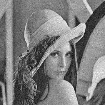
(a) Original $512\times 512$ image and noisy image with $\sigma=20$ ($22.11db$)
(b) Image denoised with our parameters ($32.39db$) and its square error
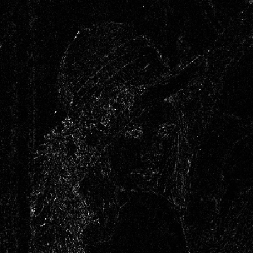
(c) Image denoised with Buade’s parameters ($31.51db$) and its square error

Figure 2: Results of denoising ”Lena” $512\times 512$ image.

5 Conclusion

We have proposed new theorems of Non-Local Means Filter, based on optimization of parameters in the weighted means approach. Our analysis shows that a small search window is preferred rather than the whole image and a large similarity patch ($m=21\times 21$) is also preferred rather than the small similarity patch ($m=7\times 7$). The proposed theorems improve the usual parameters of Non-Local Means Filter both numerically and visually in denoising performance. We hope that the convergence theorems for the Non-Local Means Filter that we deduced can also bring similar improvements for recently developed algorithms where the basic idea of the Non-Local means filter is used.

6 Proofs of the main results

6.1 Proof of Theorem 2.1

Denoting for brevity

$$I_{1} = \left(\sum_{x\in\mathbf{I}}w^{*}_{h}(x)\rho_{f,x_{0}}(x)\right)^{2}$$ (28)

$$= \left(\frac{\displaystyle\sum_{\|x-x_{0}\|_{\infty}\leq h}e^{-\frac{\rho_{f,x_{0}}^{2}(x)}{H^{2}}}{\rho}(x)}{\displaystyle\sum_{\|x-x_{0}\|_{\infty}\leq h}e^{-\frac{\rho_{f,x_{0}}^{2}(x)}{H^{2}}}}\right)^{2},$$

and

$$I_{2} = \sigma^{2}\sum_{x\in\mathbf{I}}\left(w^{*}_{h}(x)\right)^{2}$$ (29)

$$= \sigma^{2}\frac{\displaystyle\sum_{\|x-x_{0}\|_{\infty}\leq h}e^{-2\frac{\rho_{f,x_{0}}^{2}(x)}{H^{2}}}}{\left(\displaystyle\sum_{\|x-x_{0}\|_{\infty}\leq h}e^{-\frac{\rho_{f,x_{0}}^{2}(x)}{H^{2}}}\right)^{2}},$$ (30)

then we have

$$g(w^{*}_{h}(w))=I_{1}+I_{2}.$$ (31)

Noting that $te^{-\frac{t^{2}}{H^{2}}}$, $t\in[0,H/\sqrt{2})$ is increasing, it is easy to see that

$$\begin{split}&\sum_{\|x-x_{0}\|_{\infty}\leq h}e^{-\frac{L^{2}\|x-x_{0}\|_{\infty}^{2\beta}}{H^{2}}}L\|x-x_{0}\|^{\beta}_{\infty}\\ &\leq\sum_{\|x-x_{0}\|_{\infty}\leq h}L\|x-x_{0}\|^{\beta}_{\infty}e^{-\frac{L^{2}\|x-x_{0}\|_{\infty}^{2\beta}}{H^{2}}}\\ &\leq\sum_{\|x-x_{0}\|_{\infty}\leq h}L\|x-x_{0}\|^{\beta}_{\infty}\leq 4Lh^{\beta+2}n.\end{split}$$ (32)

Since $e^{-\frac{t^{2}}{H^{2}}}$, $t\in[0,H/\sqrt{2})$ is decreasing, Using one term Taylor expansion,

$$\begin{split}&\sum_{\|x-x_{0}\|_{\infty}\leq h}e^{-\frac{L^{2}\|x-x_{0}\|_{\infty}^{2\beta}}{H^{2}}}\\ &\geq\sum_{\|x-x_{0}\|_{\infty}\leq h}e^{-\frac{L^{2}\|x-x_{0}\|_{\infty}^{2\beta}}{H^{2}}}\\ &\geq\sum_{\|x-x_{0}\|_{\infty}\leq h}\left(1-\frac{L^{2}\|x-x_{0}\|_{\infty}^{2\beta}}{H^{2}}\right)\geq 2h^{2}n.\end{split}$$ (33)

The above three inequalities (28), (33) and (32) imply that

$$I_{1}\leq 4L^{2}h^{2\beta}.$$ (34)

Taking into account the inequality

$$\sum_{\|x-x_{0}\|_{\infty}\leq h}e^{-2\frac{\rho_{f,x_{0}}^{2}(x)}{H^{2}}}\leq\sum_{\|x-x_{0}\|_{\infty}\leq h}1=4h^{2}n,$$

(30) and (33), it is easily seen that

$$I_{2}\leq\frac{\sigma^{2}}{h^{2}n}.$$ (35)

Combining (31), (34), and (35), we give

$$g(w_{h}^{*})\leq 4L^{2}h^{2\beta}+\frac{\sigma^{2}}{h^{2}n}.$$ (36)

Let $h$ minimize the latter term of the above inequality. Then

$$8\beta L^{2}h^{2\beta-1}-\frac{2\sigma^{2}}{h^{3}n}=0$$

from which we infer that

$$h=\left(\frac{\sigma^{2}}{4\beta L^{2}}\right)^{\frac{1}{2\beta+2}}n^{-\frac{1}{2\beta+2}}.$$ (37)

Substituting (37) to (36) leads to

$$g(w_{h}^{*})\leq\frac{2^{\frac{2\beta+6}{2\beta+2}}\sigma^{\frac{4\beta}{2\beta+2}}L^{\frac{4}{2\beta+2}}}{\beta^{\frac{2\beta}{2\beta+2}}}n^{-\frac{2\beta}{2\beta+2}}.$$

Therefore (12) implies (15).

6.2 Proof of Theorem 2.2

First, we prove the following lemma:

Lemma 1

Suppose that $S(x)$ is given by (19), then there are two constants $c_{2}$ and $c_{3}$, such that for any $0\leq z\leq c_{2}m^{1/2},$

$$\mathbb{P}\left(\left|S(x)\right|\geq z\sqrt{m}\right)\leq 2\exp\left(-c_{3}z^{2}\right).$$

Proof

Let $m$ is given by (6). Denote $\xi\left(y\right)=\zeta\left(y\right)^{2}-2\sigma^{2}+2\Delta_{x_{0},x}\left(y\right)\zeta\left(y\right).$ Since $\zeta\left(y\right)$ is a normal random variable with mean $0$ and variance $2\sigma^{2}$, there exist two positive constants $t_{0}$ and $c_{4}$ depending only on $\beta,$ $L$, and $\sigma^{2}$ such that $\phi_{y}\left(t\right)=Ee^{t\xi(y)}\leq c_{4},$ for any $\left|t\right|\leq t_{0}.$ Let $\psi_{y}(t)=\ln\phi_{y}\left(t\right)$ be the cumulant generating function. By Chebyshev’s exponential inequality we get

$$\mathbb{P}\{S(x)>z\sqrt{m}\}\leq\exp\left(-t\sqrt{m}z+\sum_{y\in\mathbf{U}_{x_{0},\eta}}\psi_{y}(t)\right),$$ (38)

for any $\left|t\right|\leq t_{0}$ and for any $z>0.$ By three term Taylor expansion, for $\left|t\right|\leq t_{0},$

$$\psi_{y}(t)=\psi_{y}(0)+t\psi_{y}^{\prime}(0)+\frac{t^{2}}{2}\psi_{y}^{\prime\prime}{(\theta t)},$$ (39)

where $\left|\theta\right|\leq 1,$ $\psi_{y}(0)=0,$ $\psi_{y}^{\prime}(0)=\mathbb{E}\xi(y)=0$ and

$$0\leq\psi_{y}^{\prime\prime}(t)=\frac{\phi_{y}^{\prime\prime}\left(t\right)\phi_{y}\left(t\right)-\left(\phi_{y}^{\prime}\left(t\right)\right)^{2}}{\left(\phi_{y}\left(t\right)\right)^{2}}\leq\frac{\phi_{y}^{\prime\prime}\left(t\right)}{\phi_{y}\left(t\right)}.$$

Since, by Jensen’s inequality $\mathbb{E}e^{t\xi(y)}\geq e^{t\mathbb{E}\xi(y)}=1,$ we arrive at the following upper bound

$$\psi_{y}^{\prime\prime}(t)\leq\phi_{y}^{\prime\prime}\left(t\right)=\mathbb{E}\left(\xi^{2}(y)e^{t\xi(y)}\right).$$

Using the elementary inequality $x^{2}e^{x}\leq e^{3x},$ $x\geq 0,$ we have, for $\left|t\right|\leq t_{0}/3,$

$$\psi_{y}^{\prime\prime}(t) \leq \frac{9}{t_{0}^{2}}\mathbb{E}\left(\left(\frac{t_{0}}{3}\xi(y)\right)^{2}e^{\frac{t_{0}}{3}\xi(y)}\right)$$ (40)

$$\leq \frac{9}{t_{0}^{2}}\mathbb{E}e^{t_{0}\xi(y)}\leq\frac{9}{t_{0}^{2}}c_{4}.$$

The inequality (40) combining with (39) implies that for $\left|t\right|\leq t_{0},$

$$0\leq\psi_{y}(t)\leq\frac{9c_{4}}{2t_{0}^{2}}t^{2}.$$

Then (38) becomes

$$\mathbb{P}\left(S(x)>z\sqrt{m}\right)\leq\exp\left(-tz\sqrt{m}+\frac{9c_{4}}{2t_{0}^{2}}mt^{2}\right).$$

If $t=c^{\prime}z/\sqrt{m}\leq t_{0}/3$, we obtain

$$\mathbb{P}\left(S(x)>z\sqrt{m}\right)\leq\exp\left(-c^{\prime}z^{2}\left(1-\frac{9c_{4}}{2t_{0}^{2}}c^{\prime}\right)\right).$$

Choosing $c^{\prime}$ sufficiently small we arrive at

$$\mathbb{P}\left(S(x)>z\sqrt{m}\right)\leq\exp\left(-c_{3}z^{2}\right),$$

for some constant $c_{3}>0.$ In the same way we show that

$$\mathbb{P}\left(S(x)<-z\sqrt{m}\right)\leq\exp\left(-c_{3}z^{2}\right).$$

This proves the lemma.

Finally, we turn to the proof of Theorem 2.2. Applying Lemma 1 with $z=\sqrt{\frac{1}{c_{3}}\ln n^{2}}$, we see that

$$\mathbb{P}\left(\frac{1}{m}\left|S(x)\right|\geq\frac{\sqrt{\frac{1}{c_{3}}\ln n^{2}}}{\sqrt{m}}\right)\leq 2\exp\left(-\ln n^{2}\right)=\frac{2}{n^{2}}.$$

From this inequality we easily deduce that

$$\mathbb{P}\left(\max_{x\in\mathbf{U}_{x_{0},h}^{\prime}}\frac{1}{m}\left|S(x)\right|\geq\frac{\sqrt{\frac{1}{c_{3}}\ln n^{2}}}{\sqrt{m}}\right)$$

$$\leq \sum_{x\in\mathbf{U}_{x_{0},h}^{\prime}}\mathbb{P}\left(\frac{1}{m}\left|S(x)\right|\geq\frac{\sqrt{\frac{1}{c_{3}}\ln n^{2}}}{\sqrt{m}}\right)\leq\frac{2}{n}.$$

Taking $m=(2N\eta+1)^{2}=c_{0}^{2}n^{1-2\alpha}$, we arrive at

$$\mathbb{P}\left(\max_{x\in\mathbf{U}_{x_{0},h}}\frac{1}{m}\left|S(x)\right|\geq c_{1}n^{\alpha-\frac{1}{2}}\right)\leq O\left(n^{-1}\right).$$ (41)

The local Hölder condition (14) implies that

$$\left|\widehat{\rho}_{x_{0}}^{2}(x)-\rho^{2}(x)\right|\leq O\left(n^{-\frac{2\beta}{2\beta+2}}\right)+\frac{1}{m}\left|S(x)\right|.$$ (42)

Combining (41) and (42), we get

$$\mathbb{P}\left(\max_{x\in\mathbf{U}_{x_{0},h}}\left|\widehat{\rho}_{x_{0}}^{2}(x)-\rho^{2}(x)\right|\geq O\left(n^{-\frac{2\beta}{2\beta+2}}\right)+c_{1}n^{\alpha-\frac{1}{2}}\right)$$ (43)

$$\leq O\left(n^{-1}\right).$$

Because the condition $\frac{(1-\beta)^{+}}{2\beta+2}<\alpha<\frac{1}{2}$ implies that

$$n^{\alpha-\frac{1}{2}}>n^{-\frac{2\beta}{2\beta+2}},$$ (44)

the inequality (20) holds.

6.3 Proof of Theorem 3.1

Taking into account (25), (26), and the independence of $\epsilon(x)$, we have

$$\mathbb{E}\left(|\widehat{f}^{\prime}_{h}(x_{0})-f(x_{0})|^{2}\big{|}Y(x),x\in\mathbf{I}^{\prime\prime}_{x_{0}}\right)\leq g^{\prime}(\widehat{w}_{h}),$$ (45)

where

$$g^{\prime}(w)=\left(\sum_{x\in\mathbf{U}^{\prime}_{x_{0},h}}{w}(x)\rho_{f,x_{0}}(x)\right)^{2}+\sigma^{2}\sum_{x\in\mathbf{U}^{\prime}_{x_{0},h}}{w}^{2}(x).$$

From the proof of Theorem 2.1, we infer that

$$g^{\prime}(w^{\ast}_{h})\leq\frac{3}{2}\left(\frac{2^{\frac{2\beta+6}{2\beta+2}}\sigma^{\frac{4\beta}{2\beta+2}}L^{\frac{4}{2\beta+2}}}{\beta^{\frac{2\beta}{2\beta+2}}}n^{-\frac{2\beta}{2\beta+2}}\right).$$ (46)

By Theorem 2.2 and its proof, for $\widehat{\rho}^{\prime}_{x_{0}}$ defined by (25), there is a constant $c_{1}$ such that

$$\mathbb{P}\left(\max_{x\in\mathbf{U}^{\prime}_{x_{0},h}}\left|\widehat{\rho}_{x_{0}}^{{}^{\prime}2}(x)-\rho_{f,x_{0}}^{2}(x)\right|\geq c_{1}n^{\alpha-\frac{1}{2}}\sqrt{\ln n}\right)$$ (47)

$$= O\left(n^{-1}\right).$$

Let $\mathbf{B}=\left(\max_{x\in\mathbf{U}^{\prime}_{x_{0},h}}\left|\widehat{\rho}_{x_{0}}^{{}^{\prime}2}(x)-\rho_{f,x_{0}}^{2}(x)\right|\leq c_{1}n^{\alpha-\frac{1}{2}}\right)$. On the set $\mathbf{B}$, we have $\rho_{f,x_{0}}^{2}(x)-c_{1}n^{\alpha-\frac{1}{2}}<\widehat{\rho}_{x_{0}}^{{}^{\prime}2}(x)<\rho_{f,x_{0}}^{2}(x)+c_{1}n^{\alpha-\frac{1}{2}}$, from which we infer that

$$\begin{split}\widehat{w}_{h}(x)&=\frac{e^{-\frac{\widehat{\rho}_{x_{0}}^{{}^{\prime}2}(x)}{H^{2}}}}{\sum_{y\in\mathbf{U}_{x_{0},h}^{\prime}}e^{-\frac{\widehat{\rho}_{x_{0}}^{{}^{\prime}2}(y)}{H^{2}}}}\\ &\leq\frac{e^{-\frac{{\rho}_{f,x_{0}}^{2}(x)-c_{1}n^{\alpha-\frac{1}{2}}}{H^{2}}}}{\sum_{y\in\mathbf{U}_{x_{0},h}^{\prime}}e^{-\frac{{\rho}_{f,x_{0}}^{2}(y)+c_{1}n^{\alpha-\frac{1}{2}}}{H^{2}}}}\\ &\leq\frac{e^{-\frac{{\rho}_{f,x_{0}}^{2}(x)}{H^{2}}}\left(1+2\frac{c_{1}n^{\alpha-\frac{1}{2}}}{H^{2}}\right)}{\sum_{y\in\mathbf{U}_{x_{0},h}^{\prime}}e^{-\frac{{\rho}_{f,x_{0}}^{2}(y)}{H^{2}}}\left(1-\frac{c_{1}n^{\alpha-\frac{1}{2}}}{H^{2}}\right)}\\ &=\left(\frac{1+\frac{2c_{1}n^{\alpha-\frac{1}{2}}}{H^{2}}}{1-\frac{c_{1}n^{\alpha-\frac{1}{2}}}{H^{2}}}\right)w^{\ast}_{h}\end{split}$$

This implies that

$$g^{\prime}(\widehat{w}_{h})\leq\left(\frac{1+\frac{2c_{1}n^{\alpha-\frac{1}{2}}}{H^{2}}}{1-\frac{c_{1}n^{\alpha-\frac{1}{2}}}{H^{2}}}\right)^{2}g^{\prime}(w^{*}_{h}).$$

Consequently, the inequality (45) becomes

$$\mathbb{E}\left(|\widehat{f}^{\prime}_{h}(x_{0})-f(x_{0})|^{2}\big{|}Y(x),x\in\mathbf{I}^{\prime\prime}_{x_{0}},\mathbf{B}\right)$$ (48)

$$\leq \left(\frac{1+\frac{2c_{1}n^{\alpha-\frac{1}{2}}}{H^{2}}}{1-\frac{c_{1}n^{\alpha-\frac{1}{2}}}{H^{2}}}\right)^{2}g^{\prime}(w^{*}_{h}).$$

Since the function $f$ satisfies the local Hölder condition (14),

$$\mathbb{E}\left(|\widehat{f}^{\prime}_{h}(x_{0})-f(x_{0})|^{2}\big{|}Y(x),x\in\mathbf{I}^{\prime\prime}_{x_{0}}\right)<g^{\prime}(\widehat{w}_{h})\leq c_{2},$$ (49)

for a constant $c_{2}>0$ depending only on $\beta$, $L$, and $\sigma$. Combining (20), (48), and (49), we have

$$\begin{split}\mathbb{E}&\left(|\widehat{f}^{\prime}_{h}(x_{0})-f(x_{0})|^{2}\big{|}Y(x),x\in\mathbf{I}^{\prime\prime}_{x_{0}},\right)\\ =&\mathbb{E}\left(|\widehat{f}^{\prime}_{h}(x_{0})-f(x_{0})|^{2}\big{|}Y(x),x\in\mathbf{I}^{\prime\prime}_{x_{0}},\mathbf{B}\right)\mathbb{P}(\mathbf{B})\\ &+\mathbb{E}\left(|\widehat{f}^{\prime}_{h}(x_{0})-f(x_{0})|^{2}\big{|}Y(x),x\in\mathbf{I}^{\prime\prime}_{x_{0}},\overline{\mathbf{B}}\right)\mathbb{P}(\overline{\mathbf{B}})\\ \leq&\left(\frac{1+\frac{2c_{1}n^{\alpha-\frac{1}{2}}}{H^{2}}}{1-\frac{c_{1}n^{\alpha-\frac{1}{2}}}{H^{2}}}\right)^{2}g^{\prime}(w^{*}_{h})+O\left(n^{-1}\right)\end{split}$$

Now, the assertion of the theorem is obtained easily if we note the inequality (46).

References

- (1) Buades, A., Coll, B., and Morel, J. SIAM Journal on Multiscale Modeling and Simulation 4(2), 490–530 (2005).
- (2) Polzehl, J. and Spokoiny, V. Probab. Theory Rel. 135(3), 335–362 (2006).
- (3) Kervrann, C. and Boulanger, J. Int. J. Comput. Vis. 79(1), 45–69 (2008).
- (4) Buades, T., Lou, Y., Morel, J., and Tang, Z. In Int. workshop on Local and Non-Local Approximation in Image Processing, 1–15, August (2009).
- (5) Katkovnik, V., Foi, A., Egiazarian, K., and Astola, J. Int. J. Comput. Vis. 86(1), 1–32 (2010).
- (6) Lou, Y., Zhang, X., Osher, S., and Bertozzi, A. J. Sci. Comput. 42(2), 185–197 (2010).
- (7) Yaroslavsky, L. P. In Springer-Verlag, Berlin, (1985).
- (8) Tomasi, C. and Manduchi, R. In Proc. Int. Conf. Computer Vision, 839–846, January 04-07 (1998).
- (9) Mahmoudi, M. and Sapiro, G. IEEE Signal. Proc. Let. 12(12), 839–842 (2005).
- (10) Bilcu, R. and Vehvilainen, M. In Proc. of SPIE Conf. on Digital Photography III, volume 6502, 65020R, (2007).
- (11) Karnati, V., Uliyar, M., and Dey, S. In IEEE International Conference on Image Processing (ICIP), 2009 16th, 3873–3876. Ieee, (2009).
- (12) Vignesh, R., Oh, B., and Kuo, C. IEEE Signal. Proc. Let. 17(3), 277–280 (2010).
- (13) Kervrann, C. and Boulanger, J. IEEE Trans. Image Process. 15(10), 2866–2878 (2006).
- (14) Chatterjee, P. and Milanfar, P. In Proc. of SPIE Conf. on Computational Imaging. Citeseer, (2008).
- (15) Buades, A., Coll, B., and Morel, J. IEEE Trans. Image Process. 15(6), 1499–1505 (2006).
- (16) Dabov, K., Foi, A., Katkovnik, V., and Egiazarian, K. IEEE Trans. Image Process. 16(8), 2080–2095 (2007).
- (17) Dabov, K., Foi, A., Katkovnik, V., and Egiazarian, K. In Proc. workshop on signal processing with adaptive sparse structured representations (SPARS 09), volume 49. Citeseer, (2009).
- (18) Thacker, N., Bromiley, P., and Manj n, J. In Proc. MIUA 2008, Dundee, Scotland,, 174–178. Citeseer, July (2008).
- (19) Donoho, D. and Johnstone, J. Biometrika 81(3), 425 (1994).
- (20) Fan, J. and Gijbels, I. In Chapman & Hall, London, (1996).
- (21) Buades, A., Coll, B., and Morel, J. Multiscale Model. Simul. 4(2), 490–530 (2006).
- (22) Salmon, J. and Le Pennec, E. In IEEE Int. Conf. Image Process. (ICIP), 2977–2980. IEEE, (2009).
- (23) Katkovnik, V., Foi, A., Egiazarian, K., and Astola, J. In Proc. XII European Signal Proc. Conf., EUSIPCO 2004, Vienna, 101–104, (2004).
- (24) Foi, A., Katkovnik, V., Egiazarian, K., and Astola, J. In Proc. 6th IMA int. conf. math. in signal process., 79–82. Citeseer.
- (25) Roth, S. and Black, M. Int. J. Comput. Vision 82(2), 205–229 (2009).
- (26) Hirakawa, K. and Parks, T. IEEE Trans. Image Process. 15(9), 2730–2742 (2006).
- (27) Jin, Q., Grama, I., and Liu, Q. Arxiv preprint arXiv:1109.5640 (2011).
- (28) Hammond, D. and Simoncelli, E. IEEE Trans. Image Process. 17(11), 2089–2101 (2008).
- (29) Aharon, M., Elad, M., and Bruckstein, A. IEEE Trans. Signal Process. 54(11), 4311–4322 (2006).