2013 \acmMonth12
Random Projections for Linear Support Vector Machines
Abstract
Let be a data matrix of rank , whose rows represent points in -dimensional space. The linear support vector machine constructs a hyperplane separator that maximizes the 1-norm soft margin. We develop a new oblivious dimension reduction technique which is precomputed and can be applied to any input matrix . We prove that, with high probability, the margin and minimum enclosing ball in the feature space are preserved to within -relative error, ensuring comparable generalization as in the original space in the case of classification. For regression, we show that the margin is preserved to -relative error with high probability. We present extensive experiments with real and synthetic data to support our theory.
category:
I.5.2 Design Methodology Classifier Design and evaluation and Feature evaluation and selectioncategory:
G.1.6 Optimization Quadratic programming modelscategory:
G.1.0 General Numerical Algorithmskeywords:
Classification, Dimensionality Reduction, Support Vector MachinesSaurabh Paul, Christos Boutsidis, Malik Magdon-Ismail, Petros Drineas, 2013. Random Projections for Linear Support Vector Machines.
A short version of this paper appeared in the 16th International Conference on Artificial Intelligence and Statistics (AISTATS 2013) [Paul et al. (2013)]. Note, that the short version of our paper [Paul et al. (2013)] does not include the details of the proofs, comparison of random projections with principal component analysis, extension of random projections for SVM regression in terms of both theory and experiments and experiments with fast SVM solver on RCV1 and Hapmap-HGDP datasets.
Christos Boutsidis acknowledges the support from XDATA program of the Defense Advanced Research Projects Agency (DARPA), administered through Air Force Research Laboratory contract FA8750-12-C-0323; Petros Drineas and Malik Magdon-Ismail are supported by NSF CCF-1016501 and NSF DMS-1008983; Saurabh Paul is supported by NSF CCF-916415.
Author’s addresses: S. Paul and M. Magdon-Ismail and P. Drineas, Computer Science Department, Rensselaer Polytechnic Institute, pauls2@rpi.edu and {magdon, drinep}@cs.rpi.edu ; C. Boutsidis, Mathematical Sciences Department, IBM T.J. Watson Research Center, cboutsi@us.ibm.com.
1 Introduction
Support Vector Machines (SVM) [Cristianini and Shawe-Taylor (2000)] are extremely popular in machine learning today. They have been used in both classification and regression. For classification, the training data set consists of points , with respective labels for . For linearly separable data, the primal form of the SVM learning problem is to construct a hyperplane which maximizes the geometric margin (the minimum distance of a data point to the hyperplane), while separating the data. For non-separable data the “soft” 1-norm margin is maximized. The dual lagrangian formulation of the classification problem leads to the following quadratic program:
| (1) | ||||
In the above formulation, the unknown lagrange multipliers are constrained to lie inside the “box constraint” , where is part of the input. In order to measure the out-of-sample performance of the SVM classifier, we can use the VC-dimension of fat-separators. Assuming that the data lie in a ball of radius , and that the hypothesis set consists of hyperplanes of width (corresponding to the margin), then the -dimension of this hypothesis set is [Vapnik (1998)]. Now, given the in-sample error, we can obtain a bound for the out-of-sample error, which is monotonic in the VC-dimension [Vapnik and Chervonenkis (1971)].
Analogous to the 1-norm soft margin formulation for SVM classification, we have a similar formulation for regression called the linear -insensitive loss SVM [Cristianini and Shawe-Taylor (2000)]. The dual problem for -insensitive loss SVM regression is formulated as:
| (2) | ||||
Here, are the Lagrange multipliers and they lie in the interval
Intuitively, if one can preserve the subspace geometry, then one should be able to preserve the performance of a distance-based algorithm. We construct dimension reduction matrices which produce -dimensional feature vectors ; the matrices do not depend on the data. We show that for the data in the dimension-reduced space, the margin of separability and the minimum enclosing ball radius are preserved, since the subspace geometry is preserved. So, an SVM with an appropriate structure defined by the margin (width) of the hyperplanes [Vapnik and Chervonenkis (1971)] will have comparable VC-dimension and, thus, generalization error. This is true for classification. The -insensitive loss SVM regression problem is an unbounded problem and as such, we are not able to infer anything related to the generalization error bounds: we can only infer the preservation of margin.
1.1 Notation and SVM Basics
denote matrices and denote column vectors; (for all ) is the standard basis, whose dimensionality will be clear from context; and is the identity matrix. The Singular Value Decomposition (SVD) of a matrix of rank is equal to where is an orthogonal matrix containing the left singular vectors, is a diagonal matrix containing the singular values , and is a matrix containing the right singular vectors. The spectral norm of is .
1.1.1 SVM Classification
Let be the matrix whose rows are the vectors , be the diagonal matrix with entries , and be the vector of lagrange multipliers to be determined by solving eqn. (1). The SVM optimization problem is
| (3) | ||||
(In the above, are vectors with the implied constant entry.) Let be an optimal solution of the above problem. The optimal separating hyperplane is given by , and the points for which , i.e., the points which appear in the expansion , are the support vectors. The geometric margin, , of this canonical optimal hyperplane is , where . The data radius is . It is this and that factor into the generalization performance of the SVM through the ratio . It is worth noting, that our results hold for the separable case as well, which amounts to setting to a large value.
1.1.2 SVM Regression
Let be the matrix whose rows are the vectors , be the n-dimensional vector with the target entries, and be the vector of lagrange multipliers to be determined by solving eqn. (2). The SVM optimization problem is
| (4) | ||||
are vectors with the implied constant entry. Let be an optimal solution of the above problem. The optimal separating hyperplane is given by and the points for which , i.e., the points which appear in the expansion , are the support vectors. The geometric margin for regression is defined in the same way as it was done for classification.
1.2 Dimension Reduction
Our goal is to study how the SVM performs under (linear) dimensionality reduction transformations in the feature space. Let be the dimension reduction matrix that reduces the dimensionality of the input from to . We will choose to be a random projection matrix (see Section 2). The transformed dataset into dimensions is given by , and the SVM optimization problem for classification becomes
| (5) | |||||
For regression, the SVM optimization problem becomes
| (6) | ||||
We will present a construction for that leverages the fast Hadamard transform. The running time needed to apply this construction to the original data matrix is . Notice that while this running time is nearly linear on the size of the original data, it does not take advantage of any sparsity in the input. In order to address this deficiency, we leverage the recent work of \citeNClark12, \citeNMeng13 and \citeNNN13, which proposes a construction for that can be applied to in time; here denotes the number of non-zero entries of and is the rank of . To the best of our knowledge, this is the first independent implementation and evaluation of this potentially ground-breaking random projection technique (a few experimental results were presented by \citeNClark12, \citeNMeng13 and \citeNNN13). All constructions for are oblivious of the data and hence they can be precomputed. Also, the generalization bounds that depend on the final margin and radius of the data will continue to hold for classification, while the bound on the margin holds for regression.
The pratical intent of using linear SVM after random projections is to reduce computational complexity of training SVM and memory. For large-scale datasets, that are too big to fit into memory (see Section 4.1.3 for details), random projections serve as a possible way to estimate out-of-sample error. Random projections reduce the computational complexity of training SVM which is evident from the experiments described in Section 4.
1.3 Our Contribution
Our main theoretical results are to show that by solving the SVM optimization problem in the projected space, we get relative-error generalization performance for SVM classification and that, we preserve the margin upto relative error for SVM regression. We briefly discuss the appropriate values of , namely the dimensionality of the dimensionally-reduced problem. If is the matrix of the randomized Hadamard transform (see Section 2 for details), then given and we set
| (7) |
The running time needed to apply the randomized Hadamard transform is . If is constructed as described in \citeNClark12, \citeNMeng13 and \citeNNN13, then given and we set
| (8) |
The running time needed to apply this transform is . If is a random sign-matrix, then given and we set
| (9) |
The running time needed to apply this transform is equal to . Finally if is a random gaussian matrix, then given and we set,
| (10) |
Our main theorem will be stated in terms of the randomized Hadamard Transform, but similar statements can be obtained for the other three transforms.
Theorem 1.1.
Let be an accuracy paramater and let be a failure probability. Let be the matrix of the randomized Hadamard Transform, with as in eqn. (7). Let and be the margins obtained by solving the SVM problems using data matrices and respectively (eqns. (3) and (5)). Let be the radius of the minimum ball enclosing all points in the full-dimensional space (rows of ) and let be the radius of the ball enclosing all points in the dimensionally-reduced space (rows of ). Then, with probability at least ,
1.4 Prior work
The work most closely related to our results is that of \citeNKrish07, which improved upon \citeNBalca01. \citeNBalca01 and \citeNBalca02 used random sampling techniques for solving the SVM classification and -insensitive loss SVM regression problem respectively, but they were not able to implement their algorithms in practice. \citeNKrish07 and \citeNKrish09 showed that by using sub-problems based on Gaussian random projections, one can obtain a solution to the SVM classification and regression problem with a margin that is relative-error close to the optimal. Their sampling complexity (the parameter in our parlance) depends on , and, most importantly, on . This bound is not directly comparable to our result, which only depends on the rank of the data manifold, and holds regardless of the margin of the original problem (which could be arbitrarily small). Our results dramatically improve the running time needed to apply the random projections; our running times are (theoretically) linear in the number of non-zero entries in , whereas \citeNKrish07 necessitates time to apply on .
Blum05 showed relative error margin preservation for linearly separable data by angle preservation between points when using random orthogonal matrix, standard gaussian matrix and the random sign matrix. We show relative-error margin preservation for non-separable data and use methods that improve running time to compute random projections. \citeNShi12 establish the conditions under which margins are preserved after random projection and show that error free margins are preserved for both binary and multi-class problems if these conditions are met. They discuss the theory of margin and angle preservation after random projections using Gaussian matrices. They show that margin preservation is closely related to acute angle preservation and inner product preservation. Smaller acute angle leads to better preservation of the angle and the inner product. When the angle is well preserved, the margin is well-preserved too. There are two main differences between their result and ours. They show margin preservation to within additive error, whereas we give margin preservation to within relative error. This is a big difference especially when the margin is small. Moreover, they analyze only the separable case. We analyze the general non-separable dual problem and give a result in terms of the norm of the weight vector. For the separable case, the norm of the weight vector directly relates to the margin. For the non-separable case, one has to analyze the actual quadratic program, and our result essentially claims that the solution in the transformed space will have comparably regularized weights as the solution in the original space.
Shi09 used hash kernels which approximately preserved inner product to design a biased approximation of the kernel matrix. The hash kernels can be computed in the number of non-zero terms of a data matrix similar to the method of \citeNClark12, \citeNMeng13 and \citeNNN13 that we employed. \citeNShi09 used random sign matrices to compute random projections which typically increase the number of non-zero terms of the data matrix. However, the method of \citeNClark12, \citeNMeng13 and \citeNNN13 takes advantage of input sparsity. \citeNShi09 showed that their generalization bounds on the hash kernel and the original kernel differed by the inverse of the product of the margin and number of datapoints. For smaller margins, this difference will be high. Our generalization bounds are independent of the original margin and hold for arbitrarily small margins.
Zhang12 developed algorithms to accurately recover the optimal solution to the original SVM optimization problem using a Gaussian random projection. They compute the dual solution provided that the data matrix has low rank. This is different from our work since we analyze the ratio of radius of the minimum enclosing ball to the margin using random projections and do not try to recover the solution.
Finally, it is worth noting that random projection techniques have been applied extensively in the compressed sensing literature, and our theorems have the same flavor to a number of results in that area. However, to the best of our knowledge, the compressed sensing literature has not investigated the 1-norm soft-margin SVM optimization problem.
2 Random Projection Matrices
Random projections are extremely popular techniques in order to deal with the curse-of-dimensionality. Let the data matrix be ( data points in ) and let (with ) be a random projection matrix. Then, the projected data matrix is ( points in ). If is carefully chosen, then all pairwise Euclidean distances are preserved with high probability. Thus, the geometry of the set of points in preserved, and it is reasonable to hope that an optimization objective such as the one that appears in SVMs will be only mildly perturbed.
There are many possible constructions for the matrix that preserve pairwise distances. The most common one is a matrix whose entries are i.i.d. standard Gaussian random variables [Dasgupta and Gupta (2003), Indyk and Motwani (1998)] –RG for short. \citeNAchli03 argued that the random sign matrix – RS for short – e.g., a matrix whose entries are set to or with equal probability, also works. \citeNLi06 used the sparse random projection matrix whose entries were set to or with probability and with probability . These constructions take time to compute .
More recently, faster methods of constructing random projections have been developed, using, for example, the Fast Hadamard Transform [Ailon and Chazelle (2006)] – FHT for short. The Hadamard-Walsh matrix for any that is a power of two is defined as
with The normalized Hadamard-Walsh matrix is , which we simply denote by . We set:
| (11) |
a rescaled product of three matrices. is a random diagonal matrix with equal to with probability . is the normalized Hadamard transform matrix. is a random sampling matrix which randomly samples columns of ; specifically, each of the columns of is independent and selected uniformly at random (with replacement) from the columns of , the identity matrix. This construction assumes that is a power of two. If not, we just pad with columns of zeros (affecting run times by at most a factor of two). The important property of this transform is that the projected features can be computed efficiently in time (see Theorem 2.1 of \citeNAilon2008 for details). An important property of (that follows from prior work) is that it preserves orthogonality.
While the randomized Hadamard transform is a major improvement over prior work, it does not take advantage of any sparsity in the input matrix. To fix this, very recent work [Clarkson and Woodruff (2013)] shows that carefully constructed random projection matrices can be applied in input sparsity time by making use of generalized sparse embedding matrices. \citeNMeng13, \citeNNN13 also use a similar construction which runs in input sparsity time. Here we describe the construction of \citeNClark12. To understand their construction of , assume that the rank of is and let Then, let , , and let be an integer (by appropriately choosing the constants). The construction starts by letting be a random hash function; then, for , let and let . The construction proceeds by creating independent matrices , such that . Each is the concatenation (stacking the rows of matrices on top of each other) of the following matrices: . The matrix is defined as follows: for each , , where is selected from uniformly at random. is a binary matrix with and all remaining entries set to zero. is an random diagonal matrix, with each diagonal entry independently set to be or with probability . Finally, let be the block diagonal matrix constructed by stacking the ’s across its diagonal and let be a permutation matrix; then, . The running time is . We will call the method of \citeNClark12 to construct a sparse embedding matrix CW.
3 Geometry of SVM is preserved under Random Projection
We now state and prove our main result, namely that solving the SVM optimization problem in the projected space results in comparable margin and data radius as in the original space. The following lemma will be crucial in our proof.
Lemma 3.1.
Fix , . Let be any matrix with orthonormal columns and let as in eqn. (11), with . Then, with probability at least ,
Proof 3.2.
Consider the matrix . Using Lemma 3 of [Drineas et al. (2011)],
holds for all with probability at least . In the above, the notation denotes the -th row of as a row vector. Applying Theorem 4 with ( [Drineas et al. (2011)], Appendix) concludes the lemma.
We now state two similar lemmas that cover two additional constructions for .
Lemma 3.3.
Let and let be any matrix with orthonormal columns. Let be a (rescaled) random sign matrix. If , then with probability at least ,
Proof 3.4.
The proof of this result is a simple application of Theorem 3.1(i) of \citeNZouzi11.
Lemma 3.5.
Let , , and let be any matrix with orthonormal columns. Let be the CW random projection matrix (see Section 2) with . Then, with probability at least ,
Proof 3.6.
The proof of this result follows from Theorem 1 of \citeNMeng13.
Lemma 3.7.
Let , , and let be any matrix with orthonormal columns. Let be the Gaussian random projection matrix with . Then with probability at least ,
Proof 3.8.
The proof of this result follows from Corollary 6 of \citeNZhang12.
Lemma 3.7 does not have the log factors as in Lemma 3.1, but Gaussian projections are slower since they require full matrix-matrix multiplications.
Theorem 3.9.
Proof 3.10.
Let , and be the vector achieving the optimal solution for the problem of eqn. (3) in Section 1. Then,
| (12) | |||||
Let be the vector achieving the optimal solution for the dimensionally-reduced SVM problem of eqn. (5) using . Using the SVD of , we get
| (13) |
Since the constraints on do not depend on the data (see eqns. (3) and (5)), it is clear that is a feasible solution for the problem of eqn. (3). Thus, from the optimality of , and using eqn. (13), it follows that
| (14) | |||||
We now analyze the second term using standard sub-multiplicativity properties and . Taking
| (15) | |||||
Combining eqns. (14) and (15), we get
| (16) |
We now proceed to bound the second term in the right-hand side of the above equation. Towards that end, we bound the difference:
We can rewrite the above inequality as ; thus,
Combining with eqn. (16), we get
| (17) |
Now recall from our discussion in Section 1 that , , , and . Then, the optimal solutions and can be expressed as follows:
| (18) | |||||
| (19) |
Combining eqns. (17), (18), and (19), we get
| (20) | |||||
Our second theorem argues that the radius of the minimum ball enclosing all projected points (the rows of the matrix ) is very close to the radius of the minimum ball enclosing all original points (the rows of the matrix ). We will prove this theorem for as in eqn. (11), but similar results can be proven for the other two constructions for .
Theorem 3.11.
Fix , . Let be the radius of the minimum ball enclosing all points in the full-dimensional space (the rows of the matrix ), and let be the radius of the ball enclosing all points in the dimensionally reduced space (the rows of the matrix ). Then, if , with probability at least ,
Proof 3.12.
We consider the matrix whose first rows are the rows of and whose last row is the vector ; here denotes the center of the minimum radius ball enclosing all points. Then, the SVD of is equal to , where , , and . Here is the rank of the matrix and clearly . (Recall that is the rank of the matrix .) Let be the radius of the minimal radius ball enclosing all points in the original space. Then, for any ,
| (22) |
Now consider the matrix and notice that
In the above, we let be the matrix that satisfies , and we also used . Now consider the ball whose center is the -st row of the matrix (essentially, the projection of the center of the minimal radius enclosing ball for the original points). Let ; then, using the above bound and eqn. (22), we get
Thus, there exists a ball centered at (the projected center of the minimal radius ball in the original space) with radius at most that encloses all the projected points. Recall that is defined as the radius of the minimal radius ball that encloses all points in projected subspace; clearly,
We can now use Lemma 3.1 on to conclude that (using )
Similar theorems can be proven for the two other constructions of by using appropriate values for . We are now ready to conclude the proof of Theorem 1.1.
Proof 3.13.
4 Experiments
In our experimental evaluations, we implemented random projections using four different methods: RG, RS, FHT, and CW (see Section 2 for definitions) in MATLAB version 7.13.0.564 (R2011b). We ran the algorithms using the same values of (the dimension of the projected feature space) for all algorithms, but we varied across different datasets. We used LIBLINEAR [Fan et al. (2008)] and LIBSVM [Chang and Lin (2011)] as our linear SVM solver with default settings. In all cases, we ran our experiments on the original full data (referred to as “full” in the results), as well as on the projected data. For large-scale datasets, we use LIBLINEAR which is a faster SVM solver than LIBSVM, while for medium-scale datasets we use LIBSVM. We partitioned the data randomly for ten-fold cross-validation in order to estimate out-of-sample error. We repeated this partitioning ten times to get ten ten-fold cross-validation experiments. In the case where the dataset is already available in the form of a training and test-set, we do not perform ten-fold cross validation and use the given training and test set instead. In order to estimate the effect of the randomness in the construction of the random projection matrices, we repeated our cross-validation experiments ten times using ten different random projection matrices for all datasets. For classification experiments, we report in-sample error (), out-of-sample error (), the time to compute random projections (), the total time needed to both compute random projections and run SVMs on the lower-dimensional problem (), and the margin (). For regression experiments, we report the margin, the combined running-time of random projections and SVM, mean-squared error and the squared correlation-coefficient of . All results are averaged over the ten cross-validation experiments and the ten choices of random projection matrices. For each of the aforementioned quantities, we report both its mean value and its standard deviation .
4.1 Experiments on SVM Classification
We describe experimental evaluations on three real-world datasets, namely a collection of document-term matrices (the TechTC-300 dataset [Davidov et al. (2004)]), a subset of the Reuters Corpus dataset (RCV1 Dataset [Lewis et al. (2004)]) and a population genetics dataset (the joint Human Genome Diversity Panel or HGDP [Li et al. (2008)] and the HapMap Phase 3 data [Paschou et al. (2010)]) and also on three synthetic datasets. The synthetic datasets, a subset of the RCV1 dataset and the TechTC-300 dataset correspond to binary classification tasks while the joint HapMap-HGDP dataset and a subset of the RCV1 dataset correspond to multi-class classification tasks; our algorithms perform well in multi-class classification as well. For the multi-class experiments of Section 4.1.3, we do not report a margin. We use LIBLINEAR as our SVM solver for Hapmap-HGDP 111In \citeNPBMD13, the experiments on Hapmap-HGDP dataset were done using LIBSVM’s one-against-one multi-class classification method. LIBLINEAR does not have the one-against-one method implemented in the package. So we use the Crammer and Singer method [Crammer and Singer (2000)]. and the RCV1 datasets, while for the remaining datasets we use LIBSVM as our solver. For multi-class experiments, we use the method of Crammer and Singer [Crammer and Singer (2000)] implemented in LIBLINEAR.
and of Synthetic Data Projected Dimension 256 512 1024 full D1 CW 24.08 19.45 16.66 4.52 4.15 3.52 RS 24.1.0 19.46 16.36 4.45 3.79 3.22 FHT 23.52 19.59 16.67 4.21 4.05 3.37 RG 24.34 19.73 16.69 4.44 3.86 3.28 D2 CW 25.94 21.07 17.33 4.13 4.16 3.45 RS 25.80 20.80 17.47 4.40 3.93 3.42 FHT 25.33 21.23 17.58 3.69 4.24 3.53 RG 25.43 20.54 17.25 4.03 3.65 3.38 D3 CW 27.62 22.97 18.93 3.46 3.22 3.32 RS 28.15 23.00 18.72 3.02 3.48 2.78 FHT 27.92 23.41 18.73 3.46 3.60 3.02 RG 27.71 22.85 18.96 3.38 3.29 3.33 Projected Dimension 256 512 1024 full D1 CW 5.72 6.67 7.16 0.58 0.58 0.59 RS 5.73 6.66 7.18 0.57 0.55 0.55 FHT 5.76 6.64 7.15 0.56 0.58 0.56 RG 5.67 6.60 7.13 0.57 0.51 0.54 D2 CW 6.62 8.09 8.88 0.64 0.62 0.59 RS 6.65 8.10 8.88 0.64 0.60 0.63 FHT 6.66 8.06 8.84 0.63 0.65 0.63 RG 6.66 8.13 8.90 0.65 0.60 0.63 D3 CW 7.69 9.84 11.07 0.67 0.60 0.71 RS 7.61 9.85 11.05 0.59 0.6212 0.62 FHT 7.63 9.83 11.11 0.67 0.64 0.64 RG 7.69 9.85 11.04 0.67 0.61 0.7 {tabnote} \NoteSynthetic data: decreases and increases as a function of in all three families of matrices, using any of the four random projection methods. and indicate the mean and the standard deviation of over ten matrices in each family , , and , ten ten-fold cross-validation experiments, and ten choices of random projection matrices for the four methods that we investigated (a total of 1,000 experiments for each family of matrices).
4.1.1 Synthetic datasets
The synthetic datasets are separable by construction. More specifically, we first constructed a weight vector , whose entries were selected in i.i.d. trials from a Gaussian distribution of mean and standard-deviation . We experimented with the following three distributions: , , and . Then, we normalized to create . Let ; then, we set to be equal to the -th row of , while . We generated families of matrices of different dimensions. More specifically, family contained matrices in ; family contained matrices in ; and family contained matrices in . We generated ten datasets for each of the families , , and , and we report average results over the ten datasets. We set to , , and and set to 1,000 in LIBSVM for all the experiments. Tables 4.1 shows and for the three datasets , , and . is zero for all three data families. As expected, and improve as grows for all four random projection methods. Also, the time needed to compute random projections is very small compared to the time needed to run SVMs on the projected data. Figure 1 shows the combined running time of random projections and SVMs, which is nearly the same for all four random projection methods. It is obvious that this combined running time is much smaller that the time needed to run SVMs on the full dataset (without any dimensionality reduction). For instance, for , for , , and is (respectively) 6, 9, and 25 times smaller than on the full-data.
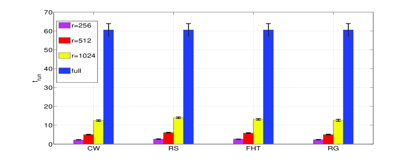
D1
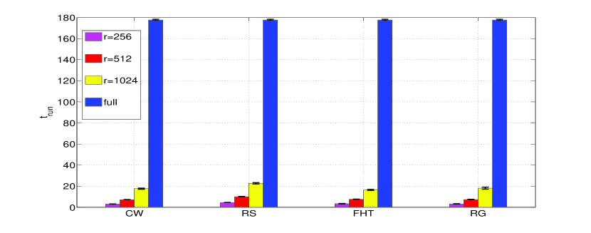 D2
D2
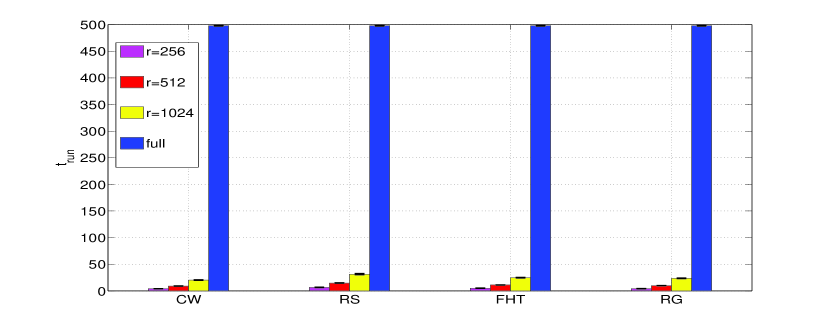 D3
D3
4.1.2 The TechTC-300 dataset
For our first real dataset, we use the TechTC-300 data, consisting of a family of 295 document-term data matrices. The TechTC-300 dataset comes from the Open Directory Project (ODP), which is a large, comprehensive directory of the web, maintained by volunteer editors. Each matrix in the TechTC-300 dataset contains a pair of categories from the ODP. Each category corresponds to a label, and thus the resulting classification task is binary. The documents that are collected from the union of all the subcategories within each category are represented in the bag-of-words model, with the words constituting the features of the data [Davidov et al. (2004)]. Each data matrix consists of 150-280 documents (the rows of the data matrix ), and each document is described with respect to 10,000-40,000 words (features, columns of the matrix ). Thus, TechTC-300 provides a diverse collection of data sets for a systematic study of the performance of the SVM on the projected versus full data.
TechTC-300 Dataset
| Projected Dimension | |||||
|---|---|---|---|---|---|
| 128 | 256 | 512 | full | ||
| CW | 24.63 | 22.84 | 21.26 | ||
| 10.57 | 10.37 | 10.17 | |||
| RS | 24.58 | 22.90 | 21.38 | ||
| 10.57 | 10.39 | 10.23 | |||
| FHT | 24.63 | 22.93 | 21.35 | ||
| 10.66 | 10.39 | 10.2 | |||
| RG | 24.59 | 22.96 | 21.36 | ||
| 10.54 | 10.5 | 10.18 | |||
| CW | 1.66 | 1.88 | 1.99 | ||
| 3.68 | 3.79 | 3.92 | |||
| RS | 1.66 | 1.88 | 1.99 | ||
| 3.65 | 3.80 | 3.91 | |||
| FHT | 1.66 | 1.88 | 1.98 | ||
| 3.65 | 3.81 | 3.88 | |||
| RG | 1.66 | 1.88 | 1.99 | ||
| 3.70 | 3.83 | 3.91 | |||
| CW | 0.0046 | 0.0059 | 0.0075 | ||
| 0.0019 | 0.0026 | 0.0033 | |||
| RS | 0.0429 | 0.0855 | 0.1719 | ||
| 0.0178 | 0.0356 | 0.072 | |||
| FHT | 0.0443 | 0.0882 | 0.1764 | ||
| 0.0206 | 0.0413 | 0.0825 | |||
| RG | 0.039 | 0.078 | 0.1567 | ||
| 0.0159 | 0.0318 | 0.0642 | |||
| CW | 1.23 | 2.22 | 4.63 | ||
| 0.87 | 0.93 | 1.93 | |||
| RS | 0.99 | 1.53 | 3.02 | ||
| 0.97 | 0.59 | 1.12 | |||
| FHT | 0.95 | 1.46 | 2.83 | ||
| 0.96 | 0.55 | 1.02 | |||
| RG | 0.82 | 1.23 | 2.48 | ||
| 0.83 | 0.45 | 0.84 | |||
TechTC300:Results on the TechTC300 dataset, averaged over 295 data matrices using four different random projection methods. The table shows how , , (in seconds), and (in seconds) depend on . and indicate the mean and the standard deviation of each quantity over 295 matrices, ten ten-fold cross-validation experiments, and ten choices of random projection matrices for the four methods that we investigated.
We set the parameter to 500 in LIBSVM for all 295 document-term matrices and set to , , and . We use a lower value of C than for the other data sets for computational reasons: larger is less efficient. We note that our classification accuracy is slightly worse (on the full data) than the accuracy presented in Section 4.4 of \citeNDavid04, because we did not fine-tune the SVM parameters as they did, since that is not the focus of this study. For every dataset and every value of we tried, the in-sample error on the projected data matched the in-sample error on the full data. We thus focus on , the margin , the time needed to compute random projections , and the total running time . We report our results averaged over 295 data matrices. Table 4.1.2 shows the behavior of these parameters for different choices of . As expected, and the margin improve as increases, and they are nearly identical for all four random projection methods. The time needed to compute random projections is smallest for CW, followed by RG, RS and FHT. As a matter of fact, for CW is ten to 20 times faster than RG, RS and FHT for different values of . This is predicted by the theory in \citeNClark12, since CW is optimized to take advantage of input sparsity. However, this advantage is lost when SVMs are applied on the dimensionally-reduced data. Indeed, the combined running time is fastest for RG, followed by FHT, RS and CW. In all cases, the total running time is smaller than the SVM running time on full dataset. For example, in the case of RG or FHT, setting achieves a running time which is about twice as fast as running SVMs on the full dataset; increases by less than .
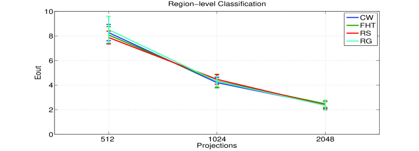
4.1.3 The HapMap-HGDP dataset
Predicting ancestry of individuals using a set of genetic markers is a well-studied classification problem. We use a population genetics dataset from the Human Genome Diversity Panel (HGDP) and the HapMap Phase 3 dataset (see \citeNPasch10 for details), in order to classify individuals into broad geographic regions, as well as into (finer-scale) populations. We study a total of 2,250 individuals from approximately 50 populations and five broad geographic regions (Asia, Africa, Europe, the Americas, and Oceania). The features in this dataset correspond to Single Nucleotide Polymorphisms (SNPs), which are well-known biallelic loci of genetic variation across the human genome. Each entry in the resulting matrix is set to (homozygotic in one allele), (homozygotic in the other allele), or (heterozygotic), depending on the genotype of the respective SNP for a particular sample. Missing entries were filled in with , , or , with probability 1/3. Each sample has a known population and region of origin, which constitute its label.
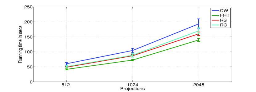
Total running time: regional classification
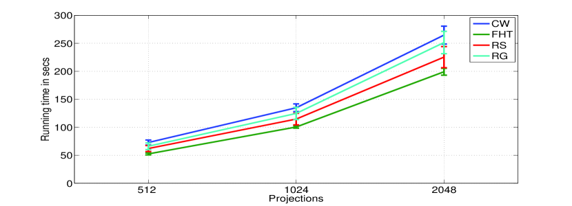
Total running time: population-level classification
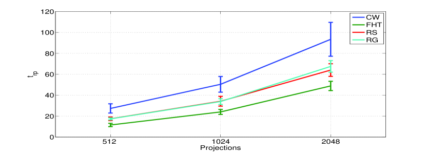
Time needed to compute random projections
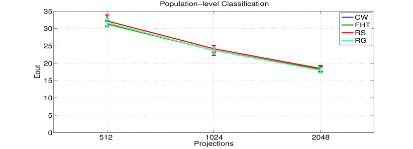
We set to , , , and in our experiments. Since this task is a multi-class classification problem, we used LIBLINEAR’s Crammer and Singer technique for classification. We ran two sets of experiments: in the first set, the classification problem is to assign samples to broad regions of origin, while in the second experiment, our goal is to classify samples into (fine-scale) populations. We set to 1,000 in LIBLINEAR for all the experiments. The in-sample error is zero in all cases. Figure 2 shows the out-of-sample error for regions and populations classification, which are nearly identical for all four random projection methods. For regional classification, we estimated to be close to , and for population-level classification, is close to . This experiment strongly supports the computational benefits of our methods in terms of main memory. is a matrix, which is too large to fit into memory in order to run SVMs. Figure 3 shows that the combined running time for four different random projection methods are nearly identical for both regions and population classification tasks. However, the time needed to compute the random projections is different from one method to the next. FHT is fastest, followed by RS, RG and CW. In this particular case, the input matrix is dense, and CW seems to be outperformed by the other methods as the running time of CW depends on the number of non-zeros of the matrix.
4.1.4 The RCV1 dataset
The RCV1 dataset [Lewis et al. (2004)]222 The RCV1 dataset is available publicly at http://www.csie.ntu.edu.tw/ cjlin/libsvmtools/datasets and contains a training-set and a test-set of predesignated size. is a benchmark dataset on text categorization. We use the RCV1 dataset for both binary and multi-class classification tasks. The RCV1 binary classification dataset had one training set containing 20,242 data-points and 47,236 features. We generate ten different test-sets each containing 20,000 points and 47,236 features from the available test-set for the binary classification task. The RCV1 binary classification dataset contains CCAT and ECAT as the positive classes and GCAT and MCAT as the negative classes. Instances in both positive and negative classes are absent. The RCV1 multi-class dataset had one training set 15,564 training points with 47,236 features and ten different test-sets each containing 16,000 data points and 47,236 features were generated from the available test-set. There are 53 classes in the RCV1 multi-class dataset. We set to , and . We use LIBLINEAR as our SVM solver. We use the L2-regularized L2-loss support vector classification in the primal mode with default settings for binary classification and the method of Crammer and Singer [Crammer and Singer (2000)] for multi-class classification. We set for both multi-class classification and binary classification. The RCV1 dataset is very sparse with 0.16% non-zero entries in the binary-class dataset and 0.14% non-zero entries in the multi-class dataset.
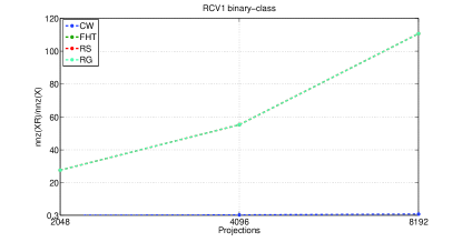
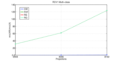
Tables 4.1.4 and 4.1.4 show the results for RCV1 binary and multi class datasets. denotes the SVM-training time on the projected data. For both binary and multi-class tasks, we observe that is close to that of full dataset and decreases with increase in number of projections. The SVM training time is smaller than that of full dataset for CW method only. For the other methods like FHT, RS and RG, the number of non-zeros in the projected data increases which increases the SVM training time. This is evident from Figure 4 which shows the ratio of number of non-zeros of projected data and full data. For all methods except CW, the number of non-zeros increases with increase in value of . This follows from the theory predicted in \citeNClark12, since CW method takes advantage of input sparsity. The combined running time is smaller than that of full-dataset for CW method. The margin of the projected data is close to that of full data for RCV1 binary class dataset.
RCV1 Dataset (Multi-class)
| Projected Dimension | |||||
|---|---|---|---|---|---|
| 2048 | 4096 | 8192 | full | ||
| CW | 18.30 | 15.15 | 13.50 | ||
| 0.157 | 0.117 | 0.079 | |||
| RS | 17.57 | 14.66 | 13.21 | ||
| 0.172 | 0.134 | 0.1094 | |||
| FHT | 17.50 | 14.58 | 13.2 | ||
| 0.2033 | 0.0905 | 0.0597 | |||
| RG | 17.47 | 14.61 | 13.21 | ||
| 0.101 | 0.146 | 0.036 | |||
| CW | 0.0093 | 0.0189 | 0.0357 | ||
| 0.0005 | 0.0007 | 0.0010 | |||
| RS | 2.412 | 4.782 | 9.49 | ||
| 0.0323 | 0.0847 | 0.0636 | |||
| FHT | 2.484 | 4.85 | 9.966 | ||
| 0.1621 | 0.023 | 0.23 | |||
| RG | 13.559 | 28.875 | 55.05 | ||
| 0.0715 | 1.9801 | 1.4315 | |||
| CW | 1.99 | 2.23 | 2.80 | ||
| 0.2309 | 0.4030 | 0.2929 | |||
| RS | 45.103 | 94.652 | 207.278 | ||
| 2.82 | 5.705 | 15.084 | |||
| FHT | 45.468 | 98.287 | 201.558 | ||
| 3.143 | 6.689 | 10.765 | |||
| RG | 47.458 | 121.208 | 263.392 | ||
| 7.222 | 23.393 | 45.814 | |||
RCV1 Multi-class: and represents the mean and standard deviation of the results which have been averaged over ten different random projection matrices. Since there was one training set, there is no standard deviation for of “full” data.
RCV1 Dataset (binary-class)
| Projected Dimension | |||||
|---|---|---|---|---|---|
| 2048 | 4096 | 8192 | full | ||
| CW | 12.90 | 9.57 | 6.54 | ||
| 1.234 | 0.619 | 0.190 | |||
| RS | 9.26 | 7.82 | 6.22 | ||
| 0.134 | 0.116 | 0.077 | |||
| FHT | 9.23 | 7.94 | 6.29 | ||
| 0.166 | 0.145 | 0.150 | |||
| RG | 9.24 | 7.75 | 6.20 | ||
| 0.255 | 0.113 | 0.109 | |||
| CW | 0.0123 | 0.0094 | 0.0125 | ||
| 0.0002 | 0.0002 | 0.0003 | |||
| RS | 0.0158 | 0.0105 | 0.0127 | ||
| 0.0005 | 0.00009 | 0.0001 | |||
| FHT | 0.0160 | 0.0105 | 0.0127 | ||
| 0.0003 | 0.0001 | 0.0001 | |||
| RG | 0.0158 | 0.0106 | 0.0127 | ||
| 0.0004 | 0.0001 | 0.00009 | |||
| CW | 0.0112 | 0.0231 | 0.0456 | ||
| 0.0008 | 0.0014 | 0.0008 | |||
| RS | 4.34 | 8.94 | 18.89 | ||
| 0.48 | 1.33 | 3.48 | |||
| FHT | 4.29 | 8.21 | 16.37 | ||
| 0.577 | 1.003 | 1.484 | |||
| RG | 20.52 | 48.18 | 86.384 | ||
| 0.248 | 3.32 | 6.15 | |||
| CW | 0.0726 | 0.1512 | 0.2909 | ||
| 0.0082 | 0.0113 | 0.009 | |||
| RS | 9.22 | 20.11 | 41.29 | ||
| 0.9396 | 3.245 | 7.3966 | |||
| FHT | 8.78 | 18.95 | 37.18 | ||
| 1.29 | 2.79 | 4.76 | |||
| RG | 11.17 | 30.17 | 44.76 | ||
| 0.364 | 4.204 | 2.079 | |||
RCV1 Binary-class: and represents the mean and standard deviation of the results which have been averaged over ten different random projection matrices. Since there was one training set, there is no standard deviation for and of “full” data.
4.2 PCA vs Random Projections
Principal Components Analysis (PCA) constructs a small number of linear features that summarize the input data. PCA is computed by first mean-centering the features of the original data and then computing a low-rank approximation of the data matrix using SVD. Thus the PCA feature matrix is given by , where represents the centered data matrix and represents the top right singular vectors of . To the best of our knowledge, there is no known theoretical framework connecting PCA with margin or generalization error of SVM, so we only provide empirical evidence of the comparison.
Our goal is to evaluate if the data matrix represented by a small number of principal components can give the same or better performance than random projections when combined with SVMs, in terms of both running time and out-of-sample error. Note that the number of random projections is always greater than the rank of the matrix. For PCA we retain a number of principal components that is less than or equal to the rank of the matrix in order to compare its performance to random projections.
We used the TechTC300 dataset for experimental evaluation and used MATLAB’s SVD solver in “econ” mode to compute PCA. We kept equal to 32, 64, and (where is the rank of the matrix) principal components. The results corresponding to a number of principal components equal to the rank of the data matrices are referred to as “full-rank”, while “full” refers to the results on the full-dimensional dataset. We ran PCA experiments on 294 datasets with , since one of them had rank less than 64. For , we used the entire set of 295 TechTC300 matrices. denotes the time to compute PCA on the dataset and we set and in our experiments. The out-of-sample error for PCA is equal to or sometimes slightly better compared to the error on the full-dimensional datasets. Even though a smaller number of principal components achieve better out-of-sample error when compared to random projections, the combined running time of SVMs and PCA is typically higher than that of random projections. The combined running time of SVMs and PCA is sensitive to the value of C, while the running time for random projections and SVM do not vary greatly, like PCA, by change of .333 We repeated all experiments on TechTC-300 using and noticed the same pattern in the results as we did for . RG and FHT are faster than the remaining two methods. Random projections are therefore a faster and more stable method than PCA. However, PCA appears to perform better than random projections when the number of components is equal to the rank of the matrix. Table 4.2 shows the results of PCA experiments; note that the standard deviation of for is quite high because of the varied running times of SVMs on the various TechTC300 matrices.
For a comparison of PCA to random projections, we consider the case of and the random gaussian matrix and randomized Hadamard Transform (see Table 4.1.2 for ), which has the best combined running time for random projections and SVMs. The combined running time of SVMs and “full-rank” PCA is smaller than that of RG (FHT) and SVMs by 0.19 (0.16) seconds, while the out-of-sample error of the former is only better. However, the time needed to compute PCA is 1.73 seconds, while random projections take negligible time to be computed; applying SVMs on the dimensionally-reduced matrix is the bottleneck of the computation. If PCA retains only 32 or 64 principal components, the running time of our method is smaller by factors of 30 and 5 respectively.
For and , SVMs and “full-rank” PCA is smaller than that of RG (FHT) and SVMs by 0.43 (0.15) seconds, while the out-of-sample error of the former is again better. For , if PCA retains only 32 or 64 principal components, the running time of our method is smaller by a few seconds.
These clearly show the advantage of using random projections over PCA, especially when a small number of principal components is desired. The PCA feature matrix is sensitive to the value of . For a higher value of , SVM takes a longer time to train the inseparable data of the PCA feature matrix.
TechTC300 PCA Experiments C=500 Projected Dimension 32 64 full-rank full PCA 15.02 17.35 17.35 9.32 9.53 9.45 PCA 1.73 1.73 1.73 1.15 1.15 1.15 PCA 86.73 14.04 2.67 174.35 81.12 1.56 C=1 Projected Dimension 32 64 full-rank full PCA 13.33 15.72 17.21 8.10 9.20 9.44 PCA 1.73 1.73 1.73 1.15 1.15 1.15 PCA 5.70 2.99 2.80 10.68 5.83 1.62 {tabnote} \NotePCA Experiments:Results on the TechTC300 dataset, averaged over all data matrices using PCA. The table shows how , (in seconds), and (in seconds) depend on . and indicate the mean and the standard deviation of each quantity over the data matrices and ten ten-fold cross-validation experiments.
4.3 Experiments on SVM regression
We describe experimental evaluations on real world datasets, namely Yalefaces dataset [Cai et al. (2006)] and a gene expression dataset (NCI60 [Ross et al. (2000)]). We convert the multi-label classification tasks into a regression problem. We use LIBSVM with default settings and use in all our experiments. The general observations from our experiments are as follows: (i) the combined runtime of random projections and SVM is smaller than the runtime of SVM on full dataset, (ii) the margin increases with an increase in the number of projections.
4.3.1 Yalefaces Dataset
The Yalefaces dataset [Cai et al. (2006)] consists of 165 grayscale images of 15 individuals. There were eleven images per subject, one per different facial expression (happy, sad, etc) or configuration (center-light, left-light, etc). The dataset has 165 datapoints and 4,096 features with 15 classes. The classes were used as the labels for regression. We set the value of to 256, 512, and 1024. for SVM and random projections is approximately 9, 7 and 4 times smaller than that of full-dataset. The margin increases as the number of random projections increases. The mean-squared in-sample error decreases with an increase in the number of random projections.
Yalefaces Dataset Projected Dimension 256 512 1024 full CW 0.2697 0.0257 0.0103 0.9859 0.9987 0.9995 RS 0.2201 0.0187 0.0107 0.9886 0.9991 0.9995 FHT 0.2533 0.0233 0.0102 0.9868 0.9988 0.9995 RG 0.281 0.0174 0.0105 0.9853 0.9991 0.9995 CW 0.11 0.12 0.13 0.0032 0.0028 0.0020 RS 0.11 0.12 0.13 0.0043 0.0024 0.0018 FHT 0.11 0.12 0.13 0.0026 0.0022 0.0031 RG 0.11 0.12 0.13 0.0034 0.0030 0.0025 CW 4.14 5.06 8.62 0.17 0.12 0.24 RS 3.92 4.81 8.45 0.17 0.10 0.19 FHT 4.12 5.09 8.69 0.23 0.17 0.25 RG 4.37 5.49 9.43 0.15 0.09 0.06 {tabnote} \NoteYalefaces Dataset:Results on the Yalefaces dataset using four different random projection methods. The table shows how , and (in seconds) depend on . and indicate the mean-squared error and the squared correlation coefficient, while and represent the mean and standard deviation over ten ten-fold cross-validation experiments, and ten choices of random projection matrices for the four methods that we investigated.
4.3.2 NCI60 Dataset
The NCI60 dataset [Ross et al. (2000)] consists of 1375 gene expression profiles of 60 human cancer cell lines. The dataset contains 1375 features and 60 datapoints with ten classes. The features contain the log-ratio of the expression levels. The classes were used as labels for regression. We set the value of to 128, 256, and 512. The running time of the four methods are nearly the same. The squared correlation-coefficient is very close to one and is not influenced by the number of projections, . The mean squared remains the same for all values of .
NCI60 Dataset Projected Dimension 128 256 512 full CW 0.0098 0.0097 0.0097 0.9987 0.9989 0.9989 RS 0.0098 0.0097 0.0097 0.9987 0.9988 0.9990 FHT 0.0097 0.0098 0.0097 0.9987 0.9988 0.9989 RG 0.0098 0.0098 0.0097 0.9987 0.9988 0.9989 CW 1.89 2.12 2.22 0.05 0.07 0.07 RS 1.90 2.09 2.25 0.10 0.06 0.07 FHT 1.88 2.10 2.22 0.10 0.09 0.05 RG 1.87 2.12 2.20 0.10 0.10 0.06 CW 0.26 0.39 0.76 0.01 0.01 0.01 RS 0.27 0.40 0.78 0.02 0.01 0.01 FHT 0.29 0.43 0.85 0.04 0.05 0.10 RG 0.26 0.38 0.74 0.02 0.04 0.05 {tabnote} \NoteNCI60 Dataset:Results on the NCI60 dataset using four different random projection methods. The table shows how , and (in seconds) depend on . See caption of Table 4.3.1 for an explanation of , , and .
5 Conclusions and open problems
We present theoretical and empirical results indicating that random projections are a useful dimensionality reduction technique for SVM classification and regression problems that handle sparse or dense data in high-dimensional feature spaces. Our theory predicts that the dimensionality of the projected space (denoted by ) has to grow essentially linearly (up to logarithmic factors) in (the rank of the data matrix) in order to achieve relative error approximations to the margin and the radius of the minimum ball enclosing the data. Such relative-error approximations imply excellent generalization performance. However, our experiments show that considerably smaller values for results in classification that is essentially as accurate as running SVMs on all available features, despite the fact that the matrices have full numerical rank. This seems to imply that our theoretical results can be improved. We implemented and tested random projection methods that work well on dense matrices (the RS and FHT methods of Section 2), as well as a very recent random projection method that works well with sparse matrices (the CW method of Section 2). We also experimented with different SVM solvers for lage and medium-scale datasets. As expected, FHT, RG and RS work well on dense data while CW is an excellent choice for sparse data, as indicated by the SVM classification experiments. For large-scale sparse data, CW is the method of choice as the other methods outweigh the benefits of performing random projections. For SVM regression experiments, the combined running times using the four methods are the same for dense datasets. The mean squared error and the squared correlation-coefficient of of the projected data are non-zero as opposed to the SVM classification experiments. Finally, we compare random projections with a popular method of dimensionality reduction, namely PCA and see that the combined running time of random projection and SVM is faster than that of SVM and PCA, with a slightly worse out-of-sample error. All our experiments are on matrices of approximately low-rank, while the theory holds for matrices of exactly low-rank. It is not known if the theory extends to matrices of approximately low rank. This is an open problem and needs further investigation.
References
- [1]
- Achlioptas (2003) D. Achlioptas. 2003. Database-friendly random projections: Johnson-Lindenstrauss with binary coins. J. Comput. System Sci. 66, 4 (2003), 671–687.
- Ailon and Chazelle (2006) N. Ailon and B. Chazelle. 2006. Approximate nearest neighbors and the fast Johnson-Lindenstrauss transform. In Proceedings of the 38th Annual ACM Symposium on Theory of Computing. 557–563.
- Ailon and Liberty (2008) N. Ailon and E. Liberty. 2008. Fast dimension reduction using Rademacher series on dual BCH codes. In Proceedings of the 19th Annual ACM-SIAM Symposium on Discrete Algorithms. 1–9.
- Balcazar et al. (2001) J.L. Balcazar, Y. Dai, and O. Watanabe. 2001. A Random Sampling Technique for Training Support Vector Machines. In Proceedings of the 12th International Conference on Algorithmic Learning Theory. 119–134.
- Balcázar et al. (2002) J.L. Balcázar, Y. Dai, and O. Watanabe. 2002. Provably Fast Support Vector Regression using Random Sampling. In In Proceedings of SIAM Workshop in Discrete Mathematics and Data Mining.
- Blum (2006) A. Blum. 2006. Random Projection, Margins, Kernels, and Feature-Selection. In In Proceedings of the International Conference on Subspace, Latent Structure and Feature Selection. 52–68.
- Cai et al. (2006) D. Cai, X. He, J. Han, and H-J. Zhang. 2006. Orthogonal Laplacianfaces for Face Recognition. IEEE Transactions on Image Processing 15, 11 (2006), 3608–3614.
- Chang and Lin (2011) C-C. Chang and C-J. Lin. 2011. LIBSVM: A library for support vector machines. ACM Transactions on Intelligent Systems and Technology 2 (2011), 27:1–27:27. Issue 3. Software available at http://www.csie.ntu.edu.tw/~cjlin/libsvm.
- Clarkson and Woodruff (2013) K.L. Clarkson and D.W. Woodruff. 2013. Low Rank Approximation and Regression in Input Sparsity Time. In Proceedings of the 45th ACM Symposium on the Theory of Computing.
- Crammer and Singer (2000) K. Crammer and Y. Singer. 2000. On the learnability and design of output codes for multi-class problems.. In In Computational Learning Theory. 35–46.
- Cristianini and Shawe-Taylor (2000) N. Cristianini and J. Shawe-Taylor. 2000. Support Vector Machines and other kernel-based learning methods. Cambridge University Press.
- Dasgupta and Gupta (2003) S. Dasgupta and A. Gupta. 2003. An elementary proof of a theorem of Johnson and Lindenstrauss. Random Structures and Algorithms 22, 1 (2003), 60–65.
- Davidov et al. (2004) D. Davidov, E. Gabrilovich, and S. Markovitch. 2004. Parameterized generation of labeled datasets for text categorization based on a hierarchical directory. In Proceedings of the 27th Annual International ACM SIGIR Conference on Research and Development in Information Retrieval. 250–257. http://techtc.cs.technion.ac.il/techtc300/techtc300.html.
- Drineas et al. (2011) P. Drineas, M.W. Mahoney, S. Muthukrishnan, and T. Sarlos. 2011. Faster least squares approximation. Numerische. Math. 117, 2 (2011), 219–249.
- Fan et al. (2008) R.-E. Fan, K.-W. Chang, C.-J. Hsieh, X.-R. Wang, and C.-J. Lin. 2008. LIBLINEAR: A library for large linear classification. Journal of Machine Learning Research (2008), 1871 –1874.
- Indyk and Motwani (1998) P. Indyk and R. Motwani. 1998. Approximate nearest neighbors: towards removing the curse of dimensionality. In Proceedings of the 30th Annual ACM Symposium on Theory of Computing. 604–613.
- Jethava et al. (2009) V. Jethava, K. Suresh, C. Bhattacharyya, and R. Hariharan. 2009. Randomized Algorithms for Large scale SVMs. CoRR abs/0909.3609 (2009). http://arxiv.org/abs/0909.3609.
- Krishnan et al. (2008) S. Krishnan, C. Bhattacharyya, and R. Hariharan. 2008. A Randomized Algorithm for Large Scale Support Vector Learning. In Advances in 20th Neural Information Processing Systems. 793–800.
- Lewis et al. (2004) D. D. Lewis, Y. Yang, T. G. Rose, and F. Li. 2004. RCV1: A new benchmark collection for text categorization research. Journal of Machine Learning Research (2004), 361–397.
- Li et al. (2008) J.Z. Li, D.M. Absher, H. Tang, A.M. Southwick, A.M. Casto, S. Ramachandran, H.M. Cann, G.S. Barsh, M. Feldman, L.L. Cavalli-Sforza, and R.M. Myers. 2008. Worldwide human relationships inferred from genome-wide patterns of variation. Science 319, 5866 (2008), 1100–1104.
- Li et al. (2006) P. Li, T.J. Hastie, and W.K. Church. 2006. Very sparse random projections. In Proceedings of the 12th ACM SIGKDD International Conference on Knowledge Discovery and Data Mining. 287–296.
- Magen and Zouzias (2011) A. Magen and A. Zouzias. 2011. Low rank matrix-valued Chernoff bounds and approximate matrix multiplication. In Proceedings of the 22nd Annual ACM-SIAM Symposium on Discrete Algorithms. 1422–1436.
- Meng and Mahoney (2013) X. Meng and M.W. Mahoney. 2013. Low-distortion Subspace Embeddings in Input-Sparsity Time and Applications to Robust Linear Regression. In Proceedings of the 45th ACM Symposium on the Theory of Computing.
- Nelson and Nguyen (2013) J. Nelson and H.L. Nguyen. 2013. OSNAP: Faster numerical linear algebra algorithms via sparser subspace embeddings. In Proceedings of the 54th Annual IEEE Symposium on Foundations of Computer Science (FOCS).
- Paschou et al. (2010) P. Paschou, J. Lewis, A. Javed, and P. Drineas. 2010. Ancestry informative markers for fine-scale individual assignment to worldwide populations. Journal of Medical Genetics 47, 12 (2010), 835–47.
- Paul et al. (2013) S. Paul, C. Boutsidis, M. Magdon-Ismail, and P. Drineas. 2013. Random Projections for Support Vector Machines. In Proceedings of the 16th International Conference on Artificial Intelligence & Statistics, JMLR W& CP. 498 –506.
- Ross et al. (2000) D.T. Ross, U. Scherf, M.B. Eisen, C.M. Perou, P. Spellman, V. Iyer, S.S. Jeffrey, M. Van de Rijn, M. Waltham, A. Pergamenschikov, J.C.F Lee, D. Lashkari, D. Shalon, T.G. Myers, J.N. Weinstein, D. Botstein, and P.O. Brown. 2000. Systematic Variation in Gene Expression Patterns in Human Cancer Cell Lines. Nature Genetics 24, 3 (2000), 227–234.
- Shi et al. (2009) Q. Shi, J. Petterson, G. Dror, J. Langford, A. Smola, and S.V.N. Vishwanathan. 2009. Hash Kernels for Structured Data. Journal of Machine Learning Research 10 (2009), 2615–2637.
- Shi et al. (2012) Q. Shi, C. Shen, R. Hill, and A.V.D Hengel. 2012. Is margin preserved after random projection ?. In Proceedings of 29th International Conference on Machine Learning. 591–598.
- Vapnik and Chervonenkis (1971) V.N. Vapnik and A. Chervonenkis. 1971. On the Uniform Convergence of Relative Frequencies of Events to their Probabilities. Theory of Probability and its Applications 16 (1971), 264–280.
- Vapnik (1998) V. N. Vapnik. 1998. Statistical Learning Theory. Theory of Probability and its Applications 16 (1998), 264–280.
- Zhang et al. (2013) L. Zhang, M. Mahdavi, R. Jin, and T. Yang. 2013. Recovering Optimal Solution by Dual Random Projection. In Conference on Learning Theory (COLT) JMLR W & CP, Vol. 30. 135–157. http://arxiv.org/abs/1211.3046.
October 2013December 2013