$\beta$-decay properties for neutron-rich Kr-Tc isotopes from deformed pn-QRPA calculations with realistic forces

Abstract

In this work we studied $\beta$-decay properties for deformed neutron-rich nuclei in the region Z=36-43. We use the deformed pn-QRPA methods with the realistic CD-Bonn forces, and include both the Gamow-Teller and first-forbidden types of decays in the calculation. The obtained $\beta$-decay half-lives and neutron-emission probabilities of deformed isotopes are compared with experiment as well as with previous calculations. The advantages and disadvantages of the method are discussed.

I introduction

Decay properties such as the half-lives and $\beta$-delayed neutron emission probabilities are important inputs for the simulations of the r-process nucleosynthesis which is believed to be responsible for the production of heavy elements in our universe. In order to understand the observed elements abundance, one needs measurements together with models for making accurate predictions for these global properties of atomic nuclei out to the neutron drip-lines, especially those neutron-rich nuclei along r-process paths MPK03 ; bab2 .

Recently, a group from RIKEN has performed a series of half-life measurements for the neutron-rich Kr-Tc isotopes RIKEN11 . For some of these nuclei, some differences from the previous measurement has been found, while for others, the half-lives are measured for the first time. These measurements give us more information for exotic neutron-rich nuclei and also offer us more information relevant for the r-process flow path around the A=130 peak.

These new measurements serve as good tests or constraints for theories. The theory for such calculations from gross to microscopic have been developed for decades. There have been global estimations of half-lives from the gross theories such as those in Ref. TY69 which treats the half-lives as functions of the Q-values, proton (Z) and neutron (N) numbers. More microscopic methods have been developed in Ref. MPK03 with deformed pn-QRPA methods for the Gamow-Teller (GT) type decays with the residual interaction from the phenomenological pn forces in $J^{\pi}=1^{+}$ channel. Because of the phenomenological nature of the forces designed only for the GT channel, the First-Forbidden (FF) part was estimated by gross theory instead of direct calculations MPK03 . Despite these approximations, Ref. MPK03 gives a reasonable average agreement with half-lives over the nuclear chart and for the new RIKEN data, but there are order of magnitude deviations between experiment and theory in many cases.

As an improvement, we proposed the adaption of realistic forces for the residual interactions. This method was first developed by the Tübingen group YRFS08 ; FFRS11 for $\beta\beta$-decay. The advantage of this method is that we are not restricted to GT channels. With just two parameters for the residual interactions, we can calculate all possible decay channels such as those transitions from $0^{+}$ ground states to $0^{-},1^{-},2^{-}$ final states. This gives explicit results from microscopic calculations for FF decays which in some nuclei may play an important role. On the other hand, inclusion of all spin-parities can give us better determinations of the spectra of odd-odd nuclei that makes the decay energy required for phase-space factors much more accurate. Both are advantages which can make a better prediction for $\beta$-decay properties.

This article is arranged as follows; in Sec. II we introduce the formulations of the calculations for $\beta$-decay properties and the many-body approach we adopt, in Sec. III the results and comparison to experiment and other models are discussed. The Conclusions are given in Sec. IV.

II formalism

The half-lives of $\beta$-decaying isotopes can be expressed as:

$$t_{1/2}=\ln 2/\Gamma,$$ (1)

where $\Gamma$ is the decay width and has the form:

$$\Gamma=\sum_{j}\Gamma_{j}=\sum_{j}\frac{1}{2\pi^{3}}\frac{m_{e}^{5}c^{4}}{\hbar^{7}}f_{j}(Z,R,\epsilon_{0})|M_{j}|^{2}.$$ (2)

Here the sum runs over all the possible states $j$ for the final nuclei, $f_{j}$ is the phase-space factor for state $j$, which is a function of the nucleus radius $R$, nuclear charge $Z$ and the energies of the emitted electron $\epsilon_{0}=E_{e}/m_{e}=(Q-E_{j})/m_{e}$ in unit of the electron mass $m_{e}$, while $M_{j}$ is the nuclear matrix element. In this work, we consider two kinds of decays, the Gamow-Teller (GT) and first-forbidden (FF) decays. The phase-space factors for both decays are expressed analytically in Ref. SYKO11 and references therein. The nuclear matrix elements describe the nuclear-structure part of the $\beta$-decay. They can be expressed in the form:

$$M_{j}^{I}=\langle j|O^{I}|i\rangle,$$ (3)

where $|i\rangle$ is the ground state for the parent nucleus and $O^{I}$ are the transition operators for $\beta$-decay and have different forms and selection rules for different types of decay $I$. From the expression in (2) for the half-lives for decays to each final state, one needs the information for the excitation energies of the final states and the matrix element between the initial and final states. For different type of nuclei, we will use different many-body treatments as explained below.

Various methods have been applied to this calculation each with some limitations. The large-basis shell model can account for many of the correlations, but the number of orbitals that can be considered is restricted by the computational limitations to dimensions of on the order of 10¹⁰, and in practice is used only for the Gamow-Teller decay in light nuclei ($A\leq 60$). All of the nuclei considered here are outside of this range.

Thus one needs other methods that involve various approximations. In our case, we adopt the deformed version of pn-QRPA with realistic forces as first introduced in Ref. YRFS08 . With the adiabatic Bohr-Mottelson approximation, one can prove the equivalence of the calculations performed in the laboratory systems and intrinsic systems MR90 (In the intrinsic system, the $z$ axis is attached to the symmetric axis of the nucleus). Thus we will perform our calculation in the intrinsic system without the consideration of rotations of the nucleus, and adopt the axially symmetric wave functions in the intrinsic frame. Details of the wave function calculation is described in Ref. YRFS08 as well as the treatment of BCS pairing in the deformed nuclei. With the BCS pairing, one defines the Boglyubov quasi-particle creation and annihilation operators:

$$\left(\begin{array}[]{c}\alpha^{\dagger}_{\tau}\\ \tilde{\alpha}_{\tau}\end{array}\right)=\left(\begin{array}[]{c c}u_{\tau}&v_{\tau}\\ -v_{\tau}&u_{\tau}\end{array}\right)\left(\begin{array}[]{c}c^{\dagger}_{\tau}\\ \tilde{c}_{\tau}\end{array}\right).$$ (10)

where the annihilation operators annihilate the BCS vacuum, $\alpha_{\tau}|BCS\rangle=0$. Here $c$ and $c^{\dagger}$ are single-particle annihilation and creation operators, and $u$’s and $v$’s are BCS coefficients from the solutions of BCS equation.

The intrinsic excited states $|K^{\pi},m\rangle$ are then generated by the QRPA creation operators acting on the ground states FFRS11 :

$$|K^{\pi},m\rangle = Q^{\dagger}_{K^{\pi},m}|0^{+}_{g.s.}\rangle$$

$$Q^{\dagger}_{K^{\pi},m} = \sum_{p,n}X^{m}_{pn,K^{\pi}}A^{\dagger}_{pn,K^{\pi}}-Y^{m}_{pn,K^{\pi}}\tilde{A}_{pn,K^{\pi}}.$$ (11)

Here the two quasi-particle creation and annihilation operators are defined as: $A^{\dagger}_{pn,K^{\pi}}=\alpha_{p}^{\dagger}\alpha_{\tilde{n}}^{\dagger}$ and $\tilde{A}_{pn,K^{\pi}}=\alpha_{\tilde{p}}\alpha_{n}$, with the selection rule: $K=\Omega_{p}-\Omega_{n}$. In order to obtain the forward and backward amplitudes X’s and Y’s, one needs to solve the QRPA equations:

$$\left(\begin{array}[]{c c}A(K^{\pi})&B(K^{\pi})\\ B(K^{\pi})&A(K^{\pi})\end{array}\right)\left(\begin{array}[]{c}X^{m}_{K^{\pi}}\\ -Y^{m}_{K^{\pi}}\end{array}\right)=\omega_{K^{\pi},m}\left(\begin{array}[]{c}X^{m}_{K^{\pi}}\\ -Y^{m}_{K^{\pi}}\end{array}\right).$$ (18)

The expression of matrices $A$ and $B$ and the details of the interactions are discussed in Refs. YRFS08 ; FFRS11 . The QRPA equations can be solved by diagonaliztion following the method in Ref. RS80 . The solutions contain the information of the energies from the eigenvalues and the structure information from the forward and backward amplitudes. With the states constructed from the solutions of QRPA equations, we can calculate the beta-decay half-lives. Here we briefly introduce the details of the calculations for different types of nuclei.

First, for the decays of even-even nuclei [the first even (odd) refers to the proton number Z and second even (odd) refers to the neutron number N], the parent nuclei have ground states with all the neutrons and protons paired. Thus it is the BCS vacuum with $J^{\pi}=0^{+}$. The excited states for daughter nuclei in pn-QRPA formalism are just those we constructed above, we choose the states with the lowest eigenvalues to be the ground states of the corresponding odd-odd nuclei which are the decay products. (This requires a calculation over all the possible spin projections and parities $K^{\pi}$). The excitation energies for each states are $E_{K^{\pi},m}=\omega_{K^{\pi},m}-\omega_{g.s.}$. The matrix elements of the decay to the $m$th states with spin-parity $K^{\pi}$ can then be derived as following:

$$M^{I}_{K^{\pi},m}=\langle K^{\pi},m|O^{I}_{M}|0^{+}_{g.s.}\rangle$$

$$=\sum_{pn}\delta_{KM}\langle p|O^{I}_{M}|n\rangle(X^{m}_{pn,K^{\pi}}u_{p}v_{n}+Y^{m}_{pn,K^{\pi}}v_{p}u_{n}).$$ (19)

Here $\langle p|O^{I}_{M}|n\rangle$ is the single-particle transition matrix element in the deformed basis, which can be written as a decomposition over the reduced matrix elements in spherical harmonic oscillator basis YRFS08 : $\langle p|O^{I}_{M}|n\rangle=\sum_{\eta_{p},\eta_{n}}F^{IM}_{p\eta_{p},n\eta_{n}}\langle\eta_{p}||O^{I}||\eta_{n}\rangle/\sqrt{2I+1}$. Here for GT decay the operator has the form $O^{GT}_{K}=\sigma_{K}\tau^{+}$, with the selection rules $\Delta K=0,\pm 1$ and $\Delta\pi=1$, while the expressions for the first-forbidden beta decay are more complicated with six components with different spin-parity as introduced in Ref. WM61 . We will not give the explicit expression for these components here, but mention that of which two have the selection rules $\Delta K=0$, $\Delta\pi=-1$, three have the selection rules $\Delta K=0,\pm 1$, $\Delta\pi=-1$ and one has $\Delta K=0,\pm 1,\pm 2$, $\Delta\pi=-1$.

For odd-mass nuclei, we follow the method in Ref. MPK03 , except that the $\Delta v=0$ case (defined in Ref. MR90 ), we consider only the single-particle transitions without the corrections from particle-vibration couplings for simplicity. The states of the odd-mass nuclei can be described as one corresponding quasi-particle (proton or neutron) excitation on the even-even ground states:

$$|Z\pm 1,N,i\rangle=\alpha_{p,i}^{\dagger}|Z,N,0^{+}\rangle$$

$$|Z,N\pm 1,i\rangle=\alpha_{n,i}^{\dagger}|Z,N,0^{+}\rangle,$$ (20)

or a pn-QRPA excitation state with one spectator single particle (or hole):

$$|Z+1,N,im\rangle=\alpha_{n,i}^{\dagger}|K^{\pi};m\rangle=\alpha_{n,i}^{\dagger}Q^{\dagger}_{K^{\pi},m}|Z,N,0^{+}\rangle$$

$$|Z,N-1,im\rangle=\alpha_{p,i}^{\dagger}|K^{\pi};m\rangle=\alpha_{p,i}^{\dagger}Q^{\dagger}_{K^{\pi},m}|Z,N,0^{+}\rangle.$$ (21)

Here the label $i$ is the spectator nucleon which doesn’t participate in the decay process. The ground states of these nuclei are the one quasi-particle states with the lowest quasi-particle energies $E_{\tau,0}$; here $\tau$ can be proton or neutron. Energies for the states in (20) are simply the differences between the quasi-particle energies $E=E_{i}-E_{0}$. While for the states in (21), we use different treatments for the energies as that in Ref. MPK03 : $E=Q-Q_{EE}+E_{m}$, $E_{m}$ is the actual pn-QRPA excitation energy in the even-even system and $Q-Q_{EE}$ accounts for the difference of the Q values between the odd mass isotope and the corresponding even-even one. The matrix elements for the $\Delta v=0$ single-particle transitions are then expressed as the leading order terms MR90 :

$$\langle Z+1,N,i|O^{I}_{M}|Z,N+1,0\rangle=v_{p,i}v_{n,0}\langle p,i|O^{I}_{M}|n,0\rangle$$

$$\langle Z,N-1,i|O^{I}_{M}|Z-1,N,0\rangle=u_{p,i}u_{n,0}\langle p,i|O^{I}_{M}|n,0\rangle,$$ (22)

and for the $\Delta v=1$ spectator case (also defined in Ref. MR90 ):

$$\langle Z+1,N,0m|O^{I}_{M}|Z,N+1,0\rangle$$

$$=\sum_{p,n\neq n_{0}}\delta_{KM}(X_{pn,K^{\pi}}^{m}u_{p}v_{n}+Y_{pn,K^{\pi}}^{m}v_{p}u_{n})\langle p|O^{I}_{M}|n\rangle$$

$$\langle Z,N-1,0m|O^{I}_{M}|Z-1,N,0\rangle$$

$$=\sum_{p\neq p_{0},n}\delta_{KM}(X_{pn,K^{\pi}}^{m}u_{p}v_{n}+Y_{pn,K^{\pi}}^{m}v_{p}u_{n})\langle p|O^{I}_{M}|n\rangle.$$ (23)

Here contributions from the orbit occupied by the spectator particle (hole) are excluded.

Finally, we discuss the case of odd-odd nuclei following the treatment from Fig. 3 in Ref. MR90 . In this scenario, the collective effect is excluded, and for the ground states of the odd-odd nuclei, one has simply one-neutron particle and one-proton hole acting on the even-even ground states. For the daughter even-even nuclei, the ground states are obviously the BCS vacuum, while for the excited states, there exists two different types: the first case is the two-quasiparticle excitation neglecting the collectivity, the excitation energies are: $E=E_{p,i}$ + $E_{p,0}$ (lower left panel in Fig. 3 of Ref. MR90 ) or $E=E_{n,i}$ + $E_{n,0}$ (upper right panel in Fig. 3 of Ref. MR90 ); the second case is the pn-QRPA excitation acting on the odd-odd ground, the energies are $E=Q-Q_{EE}+E_{m}$ (upper left panel in Fig. 3 of Ref. MR90 ), $Q_{EE}$ and $E_{m}$ have the same meanings as in the odd mass case. In the first case, the transition matrix elements are just those of (22) with one spectator proton hole or neutron particle. The special case is when the final states is the ground states with all neutrons and protons paired, in this case, the excitation energies are $0$ instead of $2E_{0}$(lower right panel in Fig. 3 of Ref. MR90 ).

The same matrix elements as in (23) are adopted with the exclusion of contributions from the orbits occupied by the unpaired neutron (particle) and proton (hole) of the odd-odd ground states. In this approximation, the result is independent of the odd-odd ground state spin, but the lack of collectivity will give an over-estimation on the excitation energy of the two quasi-particle final states. This makes the beta-decay Q values too low, and increases the beta lifetime. However, as discussed further below, the $\beta$-decay lifetimes for odd-odd nuclei are not so important for the r-process path.

Following the definition in Ref. MPK03 , the overall measure of error in the deviation of theory from experiment is defined by:

$$r=\log_{10}(\frac{t_{1/2,calc}}{t_{1/2,exp}})$$

$$\Sigma_{r}=[\frac{1}{n}\sum_{i=1}^{n}(r^{i})^{2}]^{1/2}$$

$$\Sigma_{r}^{10}=10^{\Sigma_{r}}$$ (24)

Here, $\Sigma_{r}^{10}$ is defined to be the total ”error”. This will be used later for quantitative estimation on the quality of calculations.

Figure 1: Illustrations of calculated branching ratios of the first-forbidden decay for different isotopes. The diagonal line indicates the approximate r-process path.

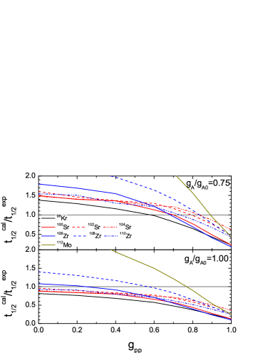
Figure 2: The half-life dependence on $g_{pp}$ for different even-even isotopes. The upper panel are results with quenched axial vector coupling constant $g_{A}=0.75g_{A0}$, while for the lower panel the bare one $g_{A0}=1.26$.

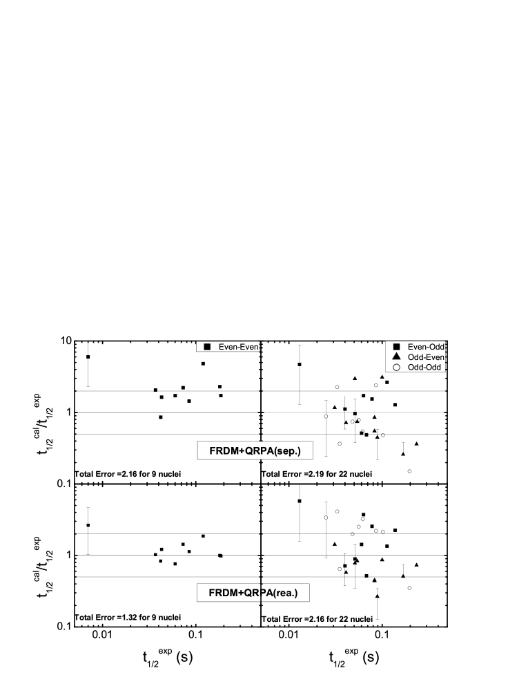
Figure 3: A comparison of the calculated half-lives from Ref. MPK03 (upper panels) and this work (lower panels) with the experimental ones from RIKEN RIKEN11 . The experimental errors are taken into account for several isotopes with large error bars. The total errors are defined in (24). The left panels are comparison for even-even isotopes, and the right panels are for other types denoted by different symbols for the three cases of (Z, N). The three horizontal lines in each panel correspond to the ratios of 2, 1 and 0.5 respectively. Here, sep. is the abbreviation for separable force and rea. for realistic force.

III results and discussion

The single-particle wave functions and energy levels are obtained by solving Schrödinger equation with the deformed Woods-Saxon potentials. The parameters of the Woods-Saxon potential are taken from Ref. NBF86 . For the choice of the model space, based on previous experience, we start from the $0\hbar\omega$ to one major shell above the Fermi surface of either proton or neutron, depending on which is close to zero-energy, so for most isotopes here with $N\leq 70$, the model space is $0-5\hbar\omega$. For the deformation parameters, we choose either the experimental ones if available (using the treatment for deformation in Ref. FFRS11 ) or those predicted by Ref. GCP09 . For the pairing interaction, we adopt the Brückner G-matrix with the Charge-dependent-Bonn force. The detailed calculation procedure and choice of parameters are described in Refs. RFSV07 ; YRFS08 ; FFRS11 . The same interaction is used as the residual interaction for pn-QRPA phonons.

As mentioned in the introduction, one of the new aspects of our work is the introduction of a microscopic calculation for the first-forbidden decays. Fig. 1 shows the region of nuclei covered in this paper. For each nucleus we show the branching ratio for the forbidden decay. They vary from several percent to at most $30\%$ in this region. Thus our discussions below apply mainly to the Gamow-Teller decay aspects of calculations. In other regions, the FF contributions are more important and an accurate determination of these decay widths can give a better accuracy, an example is given in SYKO11 for $N=126$ isotones where, for some isotones, the first forbidden decays contribute more than $80\%$ of the decay width. Overall, an explicit calculation of FF decay is required for a complete account of the beta-decay in the r-process path.

Two parameters are introduced as described in Refs. YRFS08 ; FFRS11 : the renormalized particle-hole ($g_{ph}$) and particle-particle ($g_{pp}$) strengths. However, the fitting procedure of these parameters is a bit different from Refs. YRFS08 ; FFRS11 . For the renormalized particle-hole strength $g_{ph}$, the usual way is to fit the position of the Gamow-Teller resonance. Since we don’t have enough data in the Kr-Tc region of interest, we adopt the same value as that derived in Ref. YRFS08 for double-beta decay emitter ⁷⁶Ge (In fact, the $\beta$-decay depends on the low-lying strength distributions and the choice of $g_{ph}$ does not affect the final results too much).

The calculated half-lives are sensitive to the renormalized particle-particle strength $g_{pp}$. But we must also consider the possibility of quenching of the axial-vector coupling constant due to short-range correlations and to multi-phonon effects which are excluded out in QRPA calculations. Due to the lack of experimental data on log$ft$ values of single decay branches in our mass region of interest, we take the one used in Ref. FFRS11 that was derived from experiment Guess11 for ¹⁵⁰Nd, $g_{A}=0.75g_{A0}=0.95$, where $g_{A0}=1.26$ is the bare value in the vacuum.

The relation between the calculated half-lives and values of $g_{pp}$ is illustrated in Fig. 2. When $g_{pp}$ is increased, we obtain an enhanced GT strength to low-lying states, and therefore smaller calculated half-lives. From Fig. 2, we find that without quenching, the half-lives are underestimated, and the fitted $g_{pp}$ values are around zero. If the quenching is included, realistic values from $0.6-0.9$ which reproduce the half-lives of the isotopes are obtained, which agree well with the fitted $g_{pp}$ values of $\beta\beta$-decay half-lives in Ref. FFRS11 . Due to the large uncertainty in half-life of ${}^{100}Kr$ we exclude this isotope from Fig. 1. Another isotope which is not included in the figure is ¹¹⁴Mo, because it requires a larger model space due to its neutron number $72$ (one more major shell should be added in the calculation compared with other isotopes), hence a much longer time is needed for calculation of the whole range of $g_{pp}$. However, as we shall see later, the results for ¹¹⁴Mo agree well with those obtained with the $g_{pp}$=0.75 value we choose from the fitting.

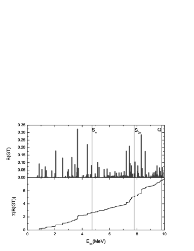
Figure 4: As an example, the low-lying GT strength distribution (upper panel) and GT running sum (lower panel) for ¹¹⁰Zr are shown. The three vertical lines correspond to $S_{n}=4.72$ MeV, $S_{2n}=7.79$ MeV and $Q=9.79$ MeV respectively, which are taken from Ref. Au02 . Here, we use $g_{pp}=0.75$, which gives a half-life $t_{1/2}=37.9$ ms and $\beta$-delayed one-neutron emission probability $P_{n}=10.5\%$.

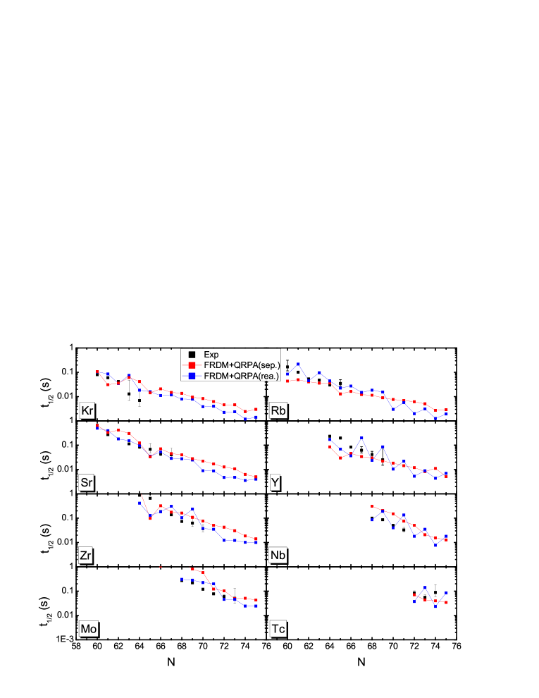
Figure 5: A comparison among the calculated half-lives from Ref. MPK03 (red), this work (blue) and measured ones (if available) with error bars from RIKEN RIKEN11 for Kr to Tc isotopes. The total errors are defined in Ref. MPK03 . Here, as before, sep. is the abbreviation for separable force and rea. for realistic forces.

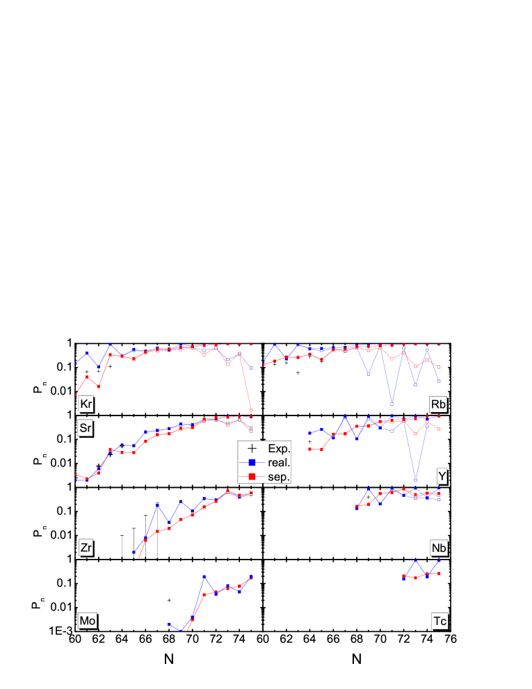
Figure 6: A comparison among the calculated $\beta$-delayed neutron emission probability $P_{n}$ values from Ref. MPK03 (red), this work (blue) and measured ones (if available) with error bars from RIKEN RIKEN11 for Kr to Tc isotopes. Here sep. is the abbreviation for separable force and rea. for realistic forces. The empty squares are the $\beta$-delayed one neutron emission probability $P_{n}$, while the solid ones are the total probability up to 3 neutron emission.

With the uncertainties of the choice of $g_{pp}$ from $0.6-0.9$, the errors of the half-lives vary by a factor of two in general. The optimal choice is $g_{pp}$=$0.75$ from the trends in the upper panel of Fig. 2. In Fig. 3, we show the ratio between calculated and measured half-lives with $g_{pp}=0.75$. Following the definition from (24), we obtain a total error of $2.1$ compared to $2.3$ in Ref. MPK03 for all nuclei from Kr to Tc. If we compare our results with those obtained in Ref. MPK03 (upper panels in Fig. 3), we find that we have a better agreement for even-even nuclei (a total error of $1.32$ compared to $2.16$ for 9 nuclei with reasonably small error bars) not simply because we have adjusted the parameters for this region, but mainly due to the adaption of excitation energies relative to the ground states of the final odd-odd nuclei. This gives a more accurate phase-space factors which effectively reduce the half-lives, and gives improved agreement with the experiment. While for Ref. MPK03 , even without the effect of quenching, there is an over-estimation for almost all even-even nuclei due to the excitation energies they choose.

As an example, we show in Fig. 4 the low-lying GT strength distributions for ¹¹⁰Zr, in order to give a general idea of how the low-lying strength is distributed, and how they contribute to the decay width in deformed nuclei. Due to the deformations, the contributions are split for $K=0$ and $K=\pm 1$ parts, not only their energies but also the strengths, this makes the distribution spread out. In Fig. 4, we show the position for Q value and the neutron separation energies. The strengths with the lowest excitation energies are most important to the decay width because of their larger phase spaces. Thus, nearly comparable amounts of GT strengths are located in the interval of $S_{n}$-$S_{2n}$ and $S_{2n}$-$Q$, but the $\beta$-delayed two neutron emission probability $P_{2n}$ is small compared with $P_{n}$. In this sense, one needs both accurate predictions for the strengths and their positions, and the advantage of realistic force is that it provides a better determination of the excitation energies. The effect of increasing $g_{pp}$ is that it enhances the low-lying strength and shifts down the excitation energies, hence reduces the half-lives. From the definition of $P_{n}$ in Refs. MPK03 ; MR90 , more low-lying strength below the neutron separation energies gives much smaller $P_{n}$ values, and vice versa. Thus, a comparison with the experiments for both the half-lives and the $P_{n}$ values is a good measure of how good the nuclear structure descriptions are.

The agreement between experiment and theory for even-odd and odd-even isotopes is about a factor of two worse than that for even-even isotopes. The lack of particle-vibration coupling in the odd-mass systems at this region does not seem to have too much affect on the final half-lives, however. This is consistent with the calculations in Ref. MPK03 , where a weak-coupling approximation was assumed.

The agreement between experiment and theory is worse for the odd-odd isotopes, and there exists a systematic overestimation for the half-lives. This is due to a shortcoming of the method we use, the lack of consideration of the collectivity for even-even daughter nuclei. This over-predicts the energies of the final states, and hence the calculated phase factors are smaller than expected. However, in spite of the shortage of the methods, we can still keep the error within an order of magnitude and for most isotopes approximately a factor of five. We note from RS12 that the r-process path does not depend strongly on the beta decay properties of the odd-odd nuclei due to their larger $S_{n}$ values. Thus, instead of improving the models for odd-odd nuclei, one alternative way is to simply use the average of the results for the neighboring odd-even and even-odd nuclei for their values in an r-process database.

With the above comparisons and discussions, we extend our calculations to all of the deformed Kr-Tc isotopes in the region $N=50-82$. We make comparisons with experimental measurement (if available) and previous theoretical predictions from Ref. MPK03 . The results are shown in Fig. 5. The same set of Q-values taken from FRDM model as used in Ref. MPK03 is adopted for the sake of comparison. One of the differences between our results and that of Ref. MPK03 is that the latter have added an extra strength spreading for each of the final states. In our calculations of even-even nuclei the strength is already spread by the deformation effects, and there is not as much motivation for adding more by hand. But for our calculations of odd-mass and odd-odd nuclei where the collective behavior has been excluded, the transitions are just between the single-particle states with little spreading compared to that in Fig. 4 for even-even nuclei. In this case, we might get better results by adding some spreading in the strength.

For most even-even isotopes, shorter half-lives by up to a factor of two are predicted in our calculation compared to Ref. MPK03 due to the lower excitation energies for the final states. This behavior applies also to some odd-mass nuclei. For even-Z isotopes, the half-lives decrease with the increase of neutrons with some small staggering behavior, but overall agreement with experiment is obtained. For odd-Z, there are systematic over estimations of the half-lives for the odd-odd isotopes with the reasons stated in Sec. II. In Ref. MPK03 , due to the additional strength spreading put in by hand, they obtained a better agreements for these isotopes. As discussed in Sec. II, the r-process results are not sensitive to the half-lives of the odd-odd nuclei, and from a practical point of view it would be adequate to simply use the average of the calculated half-lives of the neighboring even nuclei for these odd-odd nuclei.

Another observable from the experiments for some isotopes is the $P_{n}$ value, which with accurate separation energies gives a measure of the Gamow-Teller strength distribution as shown in Fig. 4. From Fig. 6, we find a good agreement again for even-even isotopes from limited data, proving that the reliability of our descriptions for deformed even-even isotopes in this region. In Fig. 6, one finds a staggering behaviours in the realistic results for the even and odd $N$ number neutrons especially for the odd-Z isotopes. The reason can be traced back to the treatment of the odd nuclei with the lack of the collectivity. This shifts the excitation energies up and the strength distributions are shifted systematically to higher energies. This behavior is more obvious for odd-odd nuclei where nearly all the strengths are shifted up. In applications of our calculations to the r-process it is preferable to replace the calculated $P_{n}$ results for odd $N$ values with the average of the neighboring even $N$ values.

IV implications for the r-process

We have investigated how the r-process element abundances are affected by the $\beta$-decay half-lives of various nuclei by changing the half-lives of Moeller’s predictionsMPK03 for all even-even or odd-odd nuclei by one order of magnitude. These preliminary results agrees with recent r-process simulations RS12 : for even-even nuclei, such changes of lifetimes have tremendous effect on the peak formations, totally change the patterns of the abundance distributions. In case of odd-odd nuclei, one order of magnitude change in all of the half-lives results in essentially the same the r-process abundance pattern except for the A=150-200 mass region where the odd-even oscillation for elemental abundances are relatively changed by about a factor of two.

We can conclude from this simple simulation that current accuracy of deformed QRPA method can meet the needs of nuclear inputs for the r-process simulation. Our next step is to extend the present calculations to other deformed regions, for example, the heavily deformed rare-earth elements region, where the beta-decay data is limited, and where it is still not understood how the the peak of rare-earth elements is formed. The final goal is to calculate the $\beta$-decay properties over the whole nuclear chart. It is also important to have reliable calculations for spherical nuclei, especially those around $N=82$ that are important for the abundance peak around $A=130$.

V conclusion

In this work, we investigated the $\beta$-decay properties of the Kr-Tc isotopes recently measured at RIKEN. With the pn-QRPA taking into account of realistic forces, a good agreement has been obtained between the theory and the experiments especially for even-even nuclei, with an accuracy within a factor of two for most of them. The current calculations provide improved results for the beta-decay half-lives of even-even nuclei. We plan to apply the present method to the rare-earth region of deformed nuclei. We also plan to use the realistic interactions for QRPA calculations of spherical nuclei. This will eventually provide an improved set of predictions for the half-lives and $P_{n}$ values that can be used in r-process network calculations for the element abundances.

This work was supported by the US NSF [PHY-0822648 and PHY-1068217]

References

- (1) P. Moller, B. Pfeiffer and K. -L. Kratz, Phys. Rev. C 67, 055802 (2003).
- (2) S. Wanajo, S. Goriely, M. Samyn and N. Itoh, Astrophys. J. 606, 1057 (2004).
- (3) S. Nishimura, Z. Li, H. Watanabe, K. Yoshinaga, T. Sumikama, T. Tachibana, K. Yamaguchi and M. Kurata-Nishimura et al., Phys. Rev. Lett. 106, 052502 (2011).
- (4) T. Suzuki, T. Yoshida, T. Kajino and T. Otsuka, Phys. Rev. C 85, 015802 (2012).
- (5) K. Takahashi and M. Yamada, Prog. Theor. Phys. 41,1470 (1969).
- (6) G. Audi, A. H. Wapstra and C. Thibault, Nucl. Phys. A 729, 337 (2002).
- (7) P. Moller and J. Randrup, Nucl. Phys. A 514, 1 (1990).
- (8) J. Krumlinde and P. Moller, Nucl. Phys. A 417, 419 (1984).
- (9) M. S. Yousef, V. Rodin, A. Faessler and F. Simkovic, Phys. Rev. C 79, 014314 (2009).
- (10) D. -L. Fang, A. Faessler, V. Rodin and F. Simkovic, Phys. Rev. C 83, 034320 (2011).
- (11) V. A. Rodin, A. Faessler, F. Simkovic and P. Vogel, Nucl. Phys. A 766, 107 (2006) [Erratum-ibid. A 793 (2007) 213].
- (12) P. Ring and P. Schuck, The Nuclear Many Body Problem (Springer-Verlag, Berlin, 1980).
- (13) H. A. Weidenmuller, Rev. Mod. Phys. 33, 574 (1961).
- (14) R. Nojarov, Z. Bochnacki and A. Faessler, Z. Phys. A324, 289 (1982).
- (15) S. Goriely, N. Chamel and J. M. Pearson, Phys. Rev. Lett. 102, 152503 (2009).
- (16) C. J. Guess, T. Adachi, H. Akimune, A. Algora, S. M. Austin, D. Bazin, B. A. Brown and C. Caesar et al., Phys. Rev. C 83, 064318 (2011).
- (17) Private communications with Rebecca Surman