Fertility Heterogeneity as a Mechanism for Power Law Distributions of Recurrence Times

Abstract

We study the statistical properties of recurrence times in the self-excited Hawkes conditional Poisson process, the simplest extension of the Poisson process that takes into account how the past events influence the occurrence of future events. Specifically, we analyze the impact of the power law distribution of fertilities with exponent $\alpha$, where the fertility of an event is the number of aftershocks of first generation that it triggers, on the probability distribution function (pdf) $f(\tau)$ of the recurrence times $\tau$ between successive events. The other input of the model is an exponential Omori law quantifying the pdf of waiting times between an event and its first generation aftershocks, whose characteristic time scale is taken as our time unit. At short time scales, we discover two intermediate power law asymptotics, $f(\tau)\sim\tau^{-(2-\alpha)}$ for $\tau\ll\tau_{c}$ and $f(\tau)\sim\tau^{-\alpha}$ for $\tau_{c}\ll\tau\ll 1$, where $\tau_{c}$ is associated with the self-excited cascades of aftershocks. For $1\ll\tau\ll 1/\nu$, we find a constant plateau $f(\tau)\simeq const$, while at long times, $1/\nu\lesssim\tau$, $f(\tau)\simeq e^{-\nu\tau}$ has an exponential tail controlled by the arrival rate $\nu$ of exogenous events. These results demonstrate a novel mechanism for the generation of power laws in the distribution of recurrence times, which results from a power law distribution of fertilities in the presence of self-excitation and cascades of triggering.

I Introduction

The statistics of ‘recurrence times’, defined as the random durations of time intervals between two consequent events, is widely used to characterize systems punctuated by short-duration occurrences interspersed between quiet phases. For instance, the statistics of recurrence times between earthquakes is the basis for hazard assessment in seismology. The statistics of recurrence times has recently been the focus of researchers interested in the properties of different natural Zaslavsky91 ; Corral2003 ; Corral2004 ; Davisenetal07 and social systems Barabasi_Nature05 ; Vasquez_et_al_06 .

The study of recurrence between earthquakes is perhaps the most advanced quantitatively due to the availability of data and the high involved stakes. The statistics of earthquake recurrence times in large geographic domains have been reported to be characterized by universal intermediate power law asymptotics, both for single homogeneous regions Bak2002 ; Corral2003 and when averaged over multiple regions Bak2002 ; Corral2004 . These intermediate power laws, as well as the scaling properties of the distribution of recurrence times, were theoretically explained by the present authors SaiSor2006 ; SaiSor2007 , using the parsimonious ETAS model of earthquakes triggering Ogata88 , which is presently the benchmark model in statistical seismology. We recall that the acronym ETAS stands for Epidemic-Type Aftershocks and the ETAS model is an incarnation of the Hawkes self-excited conditional Poisson process Hawkes1 ; Hawkes2 ; Hawkes3 ; Hawkes4 . Our previous works SaiSor2006 ; SaiSor2007 have shown that one does not need to invoke new universal laws or fancy scaling in order to explain quantitatively with high accuracy the previously reported scaling laws Bak2002 ; Corral2003 ; Bak2002 ; Corral2004 . In other words, the finding reported in Bak2002 ; Corral2003 ; Corral2004 do not contain evidence for any new physics/geophysics laws but constitute just a reformulation of the following laws:

• Earthquakes tend to trigger other earthquakes according to the same triggering mechanism, independently of their magnitudes.

• The Omori-Utsu law for aftershocks, generalized into the phenomenon of earthquake triggering where all earthquakes are treated on the same footing, states that the rate of events that are triggered by a preceding event that occurred at time $0$ decays as

  $$f_{1}(t)=\frac{\theta t_{0}^{\theta}}{(t_{0}+t)^{1+\theta}},\qquad 0<\theta\ll 1,\qquad t_{0}>0,\qquad t>0~{}.$$ (1)

  The function $f_{1}(t)$ can also be interpreted as the probability density function (pdf) of the durations of the waiting time intervals between the reference “mother” event and the triggered events of first generation corresponding to direct triggered by the mother event. The constant $t_{0}$ describes a characteristic microscopic time scale of the generalized Omori law that ensures regularization at small time and normalization.

Our previous analytical derivations SaiSor2006 ; SaiSor2007 , found in excellent agreement with empirical data Bak2002 ; Corral2003 ; Corral2004 , was essentially based on the long-memory of the Omori law (1), $f_{1}(t)\sim t^{-1-\theta}$ for large $t$ with $0\leq\theta<1$. However, it did not take into account the impact of heterogenous fertilities, which come in wildly varying values. Indeed, the number of daughters triggered by an earthquake of a given magnitude grows exponentially with its magnitude. For instance, a magnitude 8-earthquake may have tens of thousands of aftershocks of magnitude larger than 2 while a magnitude 2-earthquake may generate no more than 0.1 earthquake on average of magnitude larger than 2 Helmstteterfertility . Given the fact that the distribution of magnitudes is itself an exponentially decaying function of magnitudes (called the Gutenberg-Richter law), this translates into a heavy tail distribution of fertilities Saihelmsor05 , i.e. the distribution of the number of first generation events triggered by a given event has the following power law asymptotic:

$$p_{1}(r)\sim r^{-\alpha-1},\qquad r\to\infty,\qquad\alpha\in(1,2)~{}.$$ (2)

Precisely, $p_{1}(r)$ is the probability that the random number $R_{1}$ of first generation aftershocks triggered independently by a given mother event is equal to a given integer $r$.

In fact, the main approximation in our previous work SaiSor2006 ; SaiSor2007 was to consider that, for the estimation of the distribution of recurrence times, it is sufficient to assume that each mother event triggers at most one event, so that the power law (2) is completely irrelevant. This surprising approximation was justified by the focus on the tail of the distribution of recurrence times, for which typically only one event, among the set of events triggered by a given earthquake, does contribute.

The goal of the present paper is to reexamine this approximation and present an exact analysis of the impact of the power law form (2) of the distribution of fertilities on the distribution of the recurrence times. To make the analysis feasible and exact, we consider the case where the Omori law is no more heavy-tailed but has a shorter memory in the form of an exponential distribution, expressed by a suitable choice of time units in the form

$$f_{1}(t)=e^{-t}.$$ (3)

In addition to getting exact analytical expressions, our study of the case of an exponential memory kernel (3) is motivated by the fact that, for many applications, this is the default assumption Chavezetal05 ; BauwensHautsch09 ; Eymanetal10 ; Azizetal10 ; Aitsahaliaetal10 ; SalmonTham08 ; Filisor12 . Therefore, this parameterization has an genuine interest and intrinsic value. This exponential memory function should not be confused with the Poisson model, which has no memory. In contrast, the Hawkes process takes into account the full set of interactions between all past events and the future events, mediated by the influence function given by $f_{1}(t)$.

The main result of the present paper is the exact expression for the full distribution $f(t)$ of recurrence times that results from all the possible cascades of triggering of events over all generations. We make explicit the substantial dependence of the power law exponents characterizing the distribution $f(t)$ on the exponent $\alpha$ of the power law tail (2) for the distribution of fertilities and on the branching ratio $n$, defined as the mean number of events of first generation triggered per event:

$$n=\text{E}\left[R_{1}\right]~{}.$$ (4)

The paper is organized as follows. Section 2 present the self-excited conditional Hawkes Poisson process and the main exact equations obtained using generating probability functions. Section 3 studies the probability of quiescence within a given fixed time interval and derives different statistical properties of earthquake clusters, such as the mean number of earthquakes in clusters and their mean duration. Section 4 presents the main results concerning the probability density functions (pdf) of the waiting times between successive earthquakes. Section 5 summarizes our main results and concludes. The Appendix makes more specific the analytical model used in our derivations and describes useful statistical properties of first generation aftershocks. While we use the language of seismology and events are named ‘earthquakes’, our results obviously apply to the many natural and social-economic-financial systems in which self-excitation occurs.

II Branching model of earthquake triggering

Before discussing the statistical properties of recurrence times, let us develop the statistical description of the random number of earthquakes occurring within the time window $(t,t+\tau)$. The Hawkes model that we consider assumes that there are exogenous events (called “immigrants” in the literature on branching processes, or “noise events”), occurring spontaneously according to a Poissonian stationary flow statistics. Thus, successive instants $\dots<t_{-1}<t_{0}<t_{1}<t_{2}<\dots$ of the noise earthquakes belong to the stationary Poisson point process with mean rate $\nu=\text{const}$. Then, the Hawkes model assumes that any given noise earthquake, occurring at $\{t_{k}\}$, triggers a total of $R_{1}^{k}$ first generation earthquakes. We assume that the set of the total numbers $\{R_{1}^{k}\}$ of first generation aftershocks triggered by noise earthquakes are iid random integers, with the same generating probability function (GPF) $G_{1}(z)$. Furthermore, the distribution of waiting times $t$ between the time $t_{k}$ of a given noise earthquake and the occurrences of its aftershocks is assumed to be $f_{1}(t)$ defined by expression (3). In turn, each of the aftershocks of first generation triggered by a given noise earthquake also triggers independently its own first generation aftershocks, with the same statistical properties (same GPF) as the first generation aftershocks.

Specifically, the Hawkes self-excited conditional Poisson process is defined by the following form of the Intensity function

$$\lambda(t|H_{t},{\cal P})=\lambda_{\rm noise}(t)+\sum_{i|t_{i}<t}R_{1}^{i}~{}f(t-t_{i})~{},$$ (5)

where the history $H_{t}=\{t_{i}\}_{1\leq i\leq i_{t},~{}t_{i_{t}}\leq t<t_{i_{t}+1}}$ includes all events that occurred before the present time $t$ and the sum in expression (5) runs over all past triggered events. The set of parameters is denoted by the symbol ${\cal P}$. The term $\lambda_{\rm noise}(t)$ means that there are some external noise (or immigrant, exogenous) sources occurring according to a Poisson process with intensity $\lambda_{\rm noise}(t)$, which may be a function of time, but all other events can be both triggered by previous events and can themselves trigger their offsprings. This gives rise to the existence of many generations of events. In the sequel, we will consider only the case where $\lambda_{\rm noise}(t)=\lambda_{\rm noise}$ is constant.

Under the above definitions and assumptions, one can prove that the GPF of the total number of all earthquakes (including noise and triggered events of all generations) occurring within the time window $(t,t+\tau)$ can be expressed as a product of two terms:

$$\Theta(z;\tau)=\Theta_{\text{out}}(z;\tau)\cdot\Theta_{\text{in}}(z;\tau)~{}.$$ (6)

The first term $\Theta_{\text{out}}(z;\tau)$ is the GPF of the number of all earthquakes in $(t,t+\tau)$ triggered by noise and triggered earthquakes that occurred up to time $t$. The second term $\Theta_{\text{in}}(z;\tau)$ is the GPF of the number of all noise earthquakes that occurred within $(t,t+\tau)$ and of all earthquakes triggered in that window by events also in $(t,t+\tau)$. The factorization of $\Theta(z;\tau)$ given by expression (6) simply expresses the independence between the branching processes starting outside and within the time window $(t,t+\tau)$.

We have previously shown SaiSor2007 ; SaiSor2006a ) that $\Theta_{\text{out}}(z;\tau)$ and $\Theta_{\text{in}}(z;\tau)$ are given respectively by

$$\Theta_{\text{out}}(z;\tau)=\exp\left(\nu\int_{0}^{\infty}\left[\mathcal{G}(z;t,\tau)-1\right]dt\right)~{},$$ (7)

and

$$\Theta_{\text{in}}(z;\tau)=\exp\left(\nu\int_{0}^{\tau}\left[zG(z;\tau)-1\right]dt\right)~{},$$ (8)

where the functions $\mathcal{G}(z;t,\tau)$ and $G(z;\tau)$ satisfy the following nonlinear integral equations:

$$\begin{array}[]{c}\displaystyle G(z;\tau)=Q\left[H(z;\tau)\right]~{},\\[2.84526pt] \displaystyle H(z;\tau)=\rho(t)-zf_{1}(\tau)\otimes G(z;\tau)~{},\\[2.84526pt] \displaystyle G(z;0)=1,\qquad H(z;0)=0~{}.\end{array}$$ (9)

and

$$\begin{array}[]{c}\displaystyle\mathcal{G}(z;t,\tau)=Q[\mathcal{H}(z;t,\tau)]~{},\\[2.84526pt] \displaystyle\mathcal{H}(z;t,\tau)=\rho(t+\tau)-\mathcal{G}(z;t,\tau)\otimes f_{1}(t)-zG(z;\tau)\otimes f_{1}(t+\tau)~{},\\[2.84526pt] \displaystyle\mathcal{G}(z;0,\tau)=G(z;\tau),\qquad\mathcal{H}(z;0,\tau)=H(z;\tau)~{}.\end{array}$$ (10)

The symbol $\otimes$ represents the convolution operator with respect to the repeating time arguments $t$ or $\tau$. We have introduced the auxiliary function

$$Q(y):=G_{1}(1-y)~{},$$ (11)

and the cumulative distribution function (cdf) of the first generation aftershocks instants

$$\rho(t)=\int_{0}^{t}f_{1}(t^{\prime})dt^{\prime}~{}.$$ (12)

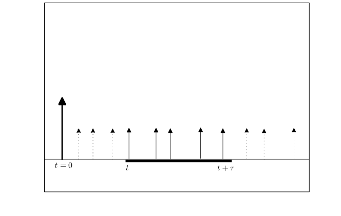
Figure 1: Schematic illustration of the geometric sense of function $\mathcal{G}(z;t,\tau)$. It is the GPF of the random number $R(t,\tau)$ of all generations aftershocks within the window $(t,t+\tau)$ triggered by a noise earthquake that occurred at the origin of time $t=0$ (large solid arrow). The aftershocks within $(t,t+\tau)$ are depicted by the small solid arrows. The aftershocks triggered outside the window $(t,t+\tau)$ are depicted by the small dotted arrows. In the picture, $R(t,\tau)=5$.

The functions $G(z;\tau)$ and $\mathcal{G}(z;t,\tau)$ have an intuitive geometric sense, illustrated by figure 1. $G(z;\tau)$ is the GPF of the random number of aftershocks of all generations triggered till the current time $t=\tau$ by some noise earthquake (or some aftershock) that occurred at the origin of time $t=0$. In turn, $\mathcal{G}(z;t,\tau)$ is the GPF of the random number of all generations aftershocks triggered within the window $(t,t+\tau)$ (for $t>0$) by some noise earthquake that occurred at the origin of time. The GPFs $G(z;\tau)$ and $\mathcal{G}(z;t,\tau)$ are related by their definition as follows:

$$G(z;0,\tau)=G(z;\tau).$$ (13)

A key input of the theory within the formalism of GPF is thus $G_{1}(y)$ or $Q(y)$ (via its definition (11)). Given expression (2), we show in the Appendix that a convenient form is

$$G_{1}(z)=1-n(1-z)+\kappa(1-z)^{\alpha},\qquad\alpha\in(1,2]~{},$$ (14)

so that the corresponding auxiliary function $Q(y)$ (11) takes the form

$$Q(y)=1-ny+\kappa y^{\alpha}~{}.$$ (15)

III Probability of quiescence, mean number of earthquakes and mean duration of clusters

III.1 Probability of quiescence

For $z=0$, relation (6) reduces to

$$\text{P}(\tau)=\text{P}_{\text{out}}(\tau)\cdot\text{P}_{\text{in}}(\tau),$$ (16)

where

$$\text{P}(\tau)=\Theta(z=0;\tau)$$ (17)

is the probability that there are no earthquakes (including the noise earthquakes and their aftershocks of all generations) within the window $(t,t+\tau)$. $\text{P}(\tau)$ can be decomposed as the product of the probability $\text{P}_{\text{in}}(\tau)$ that no noise earthquakes occur within $(t,t+\tau)$ and the probability $\text{P}_{\text{out}}(\tau)$ that no aftershocks occur within $(t,t+\tau)$ that could have been triggered by noise earthquakes and their aftershocks that occurred before and until time $t$.

In the general case, $\text{P}_{\text{in}}(\tau)$ is given by

$$\text{P}_{\text{in}}(\tau)=e^{-\nu\tau}~{}.$$ (18)

In turn, $\text{P}_{\text{out}}(\tau)=\Theta_{\text{out}}(z=0;\tau)$ by definition. Using relation (7) and equations (9), (10), we obtain

$$\text{P}_{\text{out}}(\tau)=\exp\left(\nu\int_{0}^{\infty}\left[\mathcal{G}(t,\tau)-1\right]dt\right)~{},$$ (19)

where

$$\mathcal{G}(t,\tau)=\mathcal{G}(z=0;t,\tau)$$ (20)

is defined by

$$\mathcal{G}(t,\tau)=Q[\mathcal{H}(t,\tau)]~{}.$$ (21)

The auxiliary function $\mathcal{H}(t,\tau)$ is solution of the nonlinear integral equation

$$\begin{array}[]{c}\displaystyle\mathcal{H}(t,\tau)=\rho(t+\tau)-Q[\mathcal{H}(t,\tau)]\otimes f_{1}(t)~{},\\[2.84526pt] \displaystyle\mathcal{H}(0,\tau)=\rho(\tau)~{}.\end{array}$$ (22)

III.2 Solution of equation (22) and determination of $\text{P}(\tau)$ for the exponential pdf $f_{1}(t)$

Using the exponential form of the Omori law (3), it is possible to obtain an exact analytical solution of equation (22), which gives us the possibility to explore in detail the probabilistic properties of recurrence times.

Using the form (3), it is easy to show that equation (22) reduces to the initial value problem

$$\frac{d\mathcal{H}}{dt}+\mathcal{H}+Q\left[\mathcal{H}\right]=1,\qquad\mathcal{H}(0,\tau)=\rho(\tau)~{}.$$ (23)

Using expression (15) for $Q(y)$ leads to

$$\frac{d\mathcal{H}}{dt}+(1-n)\mathcal{H}+\kappa\mathcal{H}^{\alpha}=0,\qquad\mathcal{H}(0,\tau)=\rho(\tau)~{},$$ (24)

whose solution is given by

$$\mathcal{H}(t,\tau)=\left[(1-e^{-\tau})^{1-\alpha}~{}e^{(\alpha-1)(1-n)t}+\gamma\left(e^{(\alpha-1)(1-n)t}-1\right)\right]^{1/(1-\alpha)}~{},$$ (25)

where

$$\gamma=\frac{\kappa}{1-n}~{}.$$ (26)

We have used the fact that

$$\rho(\tau)=1-e^{-\tau}~{},$$ (27)

as derived from the exponential pdf $f_{1}(t)$ given by (3) and definition (12).

We can now rewrite probability $\text{P}_{\text{out}}(\tau)$ (19) in the form

$$\text{P}_{\text{out}}(\tau)=e^{-\nu\overline{F}(\tau)}~{},$$ (28)

where

$$\overline{F}(\tau)=\int_{0}^{\infty}\left[1-\mathcal{G}(t,\tau)\right]dt~{}.$$ (29)

Taking into account expression (25) and the equality

$$\mathcal{G}(t,\tau)=Q[\mathcal{H}(t,\tau)]=1-n\mathcal{H}+\kappa\mathcal{H}^{\alpha},$$ (30)

the explicit calculation of integral (29) yields

$$\begin{array}[]{c}\displaystyle\overline{F}(\tau)=\overline{F}(n,\kappa,\alpha,\rho)=\\[5.69054pt] \displaystyle\frac{\gamma^{1/(1-\alpha)}}{(\alpha-1)(1-n)}\bigg{[}nB\left(\frac{\gamma\rho^{\alpha}}{\rho+\gamma\rho^{\alpha}},\frac{1}{\alpha-1},\frac{\alpha-2}{\alpha-1}\right)-\\[11.38109pt] \displaystyle(1-n)B\left(\frac{\gamma\rho^{\alpha}}{\rho+\gamma\rho^{\alpha}},\frac{\alpha}{\alpha-1},\frac{1}{1-\alpha}\right)\bigg{]}~{},\end{array}$$ (31)

where $\rho=\rho(\tau)$ and $B(x;a,b)$ is the incomplete beta function

$$B(x;a,b)=\int_{0}^{x}s^{a-1}(1-s)^{b-1}ds~{}.$$ (32)

In view of the key role played by the function $\overline{F}(n,\kappa,\alpha,\rho)$ in the following, it is useful to describe some of its properties. A first result of interest is its limit behavior as the branching ratio $n$ tends to $1$. Recall that this limit corresponds to the critical regime of the Hawkes process, separating the subcritical phase $n<1$ and the supercritical phase $n>1$. For $n<1$, each noise earthquake has only a finite number of aftershocks. For $n>1$, there is a non-zero probability that a single noise earthquake may generate an infinite number and infinitely long-lives sequence of aftershocks. The relevant physical regime is thus $n\leq 1$ and the boundary value $n=1$ plays a special role, especially when one remembers that $n$ can also be interpreted as the ratio of the total number of triggered events to the total number of events HelmstteterSornette03 . Hence, when $n\to 1$, most of the observed activity is endogenous, i.e., triggered by past activity.

Thus, the limit of $\overline{F}(n,\kappa,\alpha,\rho)$ as $n\to 1$ reads

$$\overline{F}(\kappa,\alpha,\rho)=\lim_{n\to 1}\overline{F}(n,\kappa,\alpha,\rho)=\frac{\rho^{2-\alpha}}{\kappa(2-\alpha)}-\rho,\quad 1<\alpha<2.$$ (33)

For $n<1$, it is convenient to choose values of $\alpha$ that take the form

$$\alpha=1+\frac{1}{m}~{},$$ (34)

so that it is possible to express the function

$$\mathcal{F}_{m}(n,\kappa,\rho)=\overline{F}\left(n,\kappa,1+\frac{1}{m},\rho\right)$$ (35)

under the form

$$\begin{array}[]{c}\displaystyle\mathcal{F}_{m}(n,\kappa,\rho)=\frac{n\rho}{1-n}+\\[11.38109pt] \displaystyle\frac{m}{\kappa^{m}}(n-1)^{m-1}\left[\ln\left(1+\frac{\kappa}{1-n}\rho^{1/m}\right)-\ln_{m}\left(1+\frac{\kappa}{1-n}\rho^{1/m}\right)\right]~{}.\end{array}$$ (36)

The auxiliary function $\ln_{m}(1+x)$ is defined as the sum of the first $m$ terms of the Taylor series expansion of the logarithm function $\ln(1+x)$ with respect to $x$:

$$\ln_{m}(1+x)=-\sum_{k=1}^{m}\frac{(-x)^{k}}{k}~{}.$$ (37)

For $m=1$ ($\alpha=2$), we have

$$\mathcal{F}_{1}(n,\kappa,\rho)=\frac{1}{\kappa}\ln\left[1+\frac{\kappa\rho}{1-n}\right]-\rho~{}.$$ (38)

For $m=2$ ($\alpha=3/2$), we have

$$\begin{array}[]{c}\displaystyle\mathcal{F}_{2}(n,\kappa,\rho)=\frac{2}{\kappa}\sqrt{\rho}-\rho-\frac{2}{\kappa^{2}}(1-n)\ln\left(1+\frac{\kappa\sqrt{\rho}}{1-n}\right)~{}.\end{array}$$ (39)

For $m=3$ ($\alpha=4/3$), we have

$$\begin{array}[]{c}\displaystyle\mathcal{F}_{3}(n,\kappa,\rho)=-\frac{3}{\kappa^{2}}(1-n)\rho^{1/3}+\frac{3}{2\kappa}~{}\rho^{2/3}-\rho+\\[11.38109pt] \displaystyle\frac{3}{\kappa^{3}}(1-n)^{2}\ln\left(1+\frac{\kappa\rho^{1/3}}{1-n}~{}\right)~{}.\end{array}$$ (40)

III.3 Mean duration of seismic clusters

III.3.1 Seismic clusters of all types

Let us consider the random duration $\Delta_{k}$ of the aftershock cluster triggered by the $k$th noise earthquake that occurred at time $t_{k}$. By definition,

$$\Delta_{k}=t_{\text{last}}^{k}-t_{k}~{},$$ (41)

where $t_{\text{last}}^{k}$ is the occurrence time of the last of its triggered aftershocks over all generations. The mean value of $\Delta_{k}$ is by definition $\langle\Delta\rangle=\int_{0}^{\infty}\varrho\cdot w(\varrho)d\varrho$, where $w(\varrho)$ is the pdf of the random cluster durations $\{\Delta_{k}\}$.

By hypothesis, the instants $\{t_{k}\}$ of the noise earthquakes form a Poissonian point process with mean rate $\nu$. Moreover, within the Hawkes branching process model, the clusters durations $\{\Delta_{k}\}$ are iid random variables. One can easily show that the probability $\text{P}_{\text{out}}(\tau)$ given by (28), that no aftershocks occur within $(t,t+\tau)$ that could have been triggered by noise earthquakes and their aftershocks that occurred before and until time $t$, take the following value in the limit $\tau\to+\infty$:

$$\text{P}_{\text{out}}(\infty)=e^{-\nu\langle\Delta\rangle}~{},$$ (42)

Thus, $\text{P}_{\text{out}}(\infty)$ is the probability that all noise earthquakes that occurred up to time $t$ do not trigger any aftershock after $t$. It follows from relation (28) and (42) that

$$\langle\Delta\rangle=\overline{F}_{\infty}(n,\kappa,\alpha,\rho=1)~{}.$$ (43)

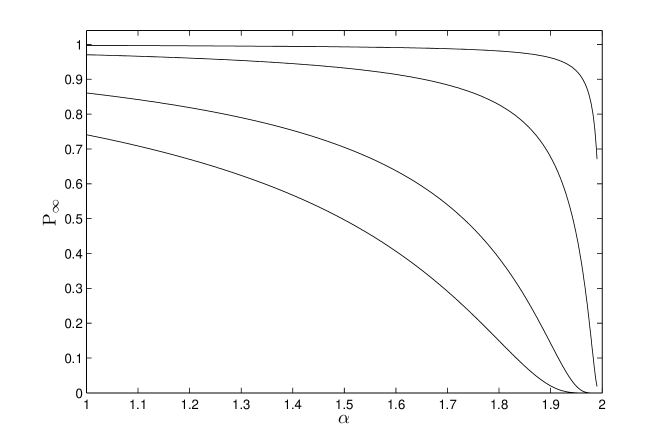
Figure 2: Dependence with respect to the exponent $\alpha$ of the probability $\text{P}_{\text{out}}(\infty)$ (42) that no aftershocks occur within $(t,t+\tau)$ that could have been triggered by noise earthquakes and their aftershocks that occurred before and until time $t$. The plot corresponds to the critical case $n=1$ with $\kappa=0.25$. Bottom to top: $\nu=0.1;0.05;0.01;0.001$.

Now, $\overline{F}_{\infty}(n,\kappa,\alpha,\rho=1)$ can be obtained as the value of the function $\overline{F}(\tau)$ given by (31) at $\tau\to+\infty$:

$$\overline{F}_{\infty}(n,\kappa,\alpha,\rho)=\overline{F}(\infty)~{}.$$ (44)

We obtain

$$\begin{array}[]{c}\displaystyle\overline{F}(n,\kappa,\alpha,\rho=1)=\\[11.38109pt] \displaystyle\frac{\gamma^{1/(1-\alpha)}}{(\alpha-1)(1-n)}\bigg{[}nB\left(\frac{\kappa}{\kappa+1-n},\frac{1}{\alpha-1},\frac{\alpha-2}{\alpha-1}\right)-\\[11.38109pt] \displaystyle(1-n)B\left(\frac{\kappa}{\kappa+1-n},\frac{\alpha}{\alpha-1},\frac{1}{1-\alpha}\right)\bigg{]}~{}.\end{array}$$ (45)

In particular, in the critical case $n=1$, we have

$$\overline{F}(1,\kappa,\alpha,1)=\frac{1}{\kappa(2-\alpha)}-1~{},$$ (46)

and thus

$$\langle\Delta\rangle=\frac{1}{\kappa(2-\alpha)}-1,\qquad n=1,\qquad\kappa<\alpha^{-1}~{}.$$ (47)

Figure 2 shows the probability $\text{P}_{\text{out}}(\infty)$ (42) as a function of the exponent $\alpha$, in the critical case $n=1$.

III.3.2 Seismic clusters with at least $m\geq 1$ aftershock

The mean duration $\langle\Delta\rangle$ of clusters given by expression (43) with (45) includes the contribution of the empty clusters for which the noise earthquake does not trigger any aftershock. It is thus interesting to evaluate another derived quantity $\langle\Delta^{1}\rangle$, defined as the mean duration of clusters that contain at least one aftershock. To get $\langle\Delta^{1}\rangle$, we divide $\langle\Delta\rangle$ by the probability that the number of aftershocks is strictly positive,

$$\langle\Delta^{1}\rangle=\langle\Delta\rangle\big{/}\text{Pr}\{R>0\}~{},$$ (48)

where $\text{Pr}\{R>0\}$ is the probability that the number $R$ of aftershocks is positive. Accordingly, one introduce the mean rate $\nu^{1}$ of the non-empty clusters equal to

$$\nu^{1}=\nu\big{/}\text{Pr}\{R>0\}~{},$$ (49)

where $\nu$ is the mean rate of noise earthquakes.

Obviously, $\text{Pr}\{R>0\}$ is given by

$$\text{Pr}\{R>0\}=1-p_{1}(0)~{},$$ (50)

where $p_{1}(0)$ is the probability that a noise earthquake does not trigger any first generation aftershock at all. Using the parameterization defined in the Appendix for the Hawkes model, $p_{1}(0)$ is given by expression (85), leading to

$$\nu^{1}=\nu\cdot(n-\kappa)\qquad\text{and}\qquad\langle\Delta^{1}\rangle=\frac{\overline{F}_{\infty}(n,\kappa,\alpha,1)}{n-\kappa}~{}.$$ (51)

In particular, in the critical case $n=1$, the mean duration of the non-empty clusters is given by

$$\langle\Delta^{1}\rangle=\frac{1-\kappa(2-\alpha)}{(2-\alpha)\kappa(1-\kappa)}~{}.$$ (52)

As an example, taking $\kappa=0.25$ and $\alpha=1.5$ yields a mean duration of the non-empty clusters in the critical case equal to $\langle\Delta^{1}\rangle\simeq 9.33$. Recall that the unit time is the characteristic decay time of the Omori law $f_{1}(t)$ (3).

This allows us to define regimes of low seismicity as characterized by the following inequalities

$$\nu\cdot\langle\Delta\rangle\ll 1\qquad\Leftrightarrow\qquad\nu^{1}\cdot\langle\Delta^{1}\rangle\ll 1~{},$$ (53)

which means that clusters are well individualized, being separated by comparatively long quiet time intervals.

It is useful to generalize the mean duration $\langle\Delta^{1}\rangle$ of clusters that contain at least one aftershock to the mean durations $\langle\Delta^{m}\rangle$ of the clusters that contain at least $m$ aftershocks. We now derive the general equation allowing one to calculate these $\langle\Delta^{m}\rangle$’s. Using the total probability formula, one can represent the pdf $w(\varrho)$ of clusters durations in the form

$$w(\varrho)=p(0)\delta(\varrho)+\sum_{j=1}^{\infty}p(j)w(\varrho|j)~{},$$ (54)

where $p(j)$ is the probability that a given noise earthquake triggers $j$ aftershocks of all generations, and $w(\varrho|j)$ is the conditional pdf of cluster durations under the condition that the number of aftershocks is equal to $j$. Accordingly, the pdf $w(\varrho|j\geqslant m)$ of the durations of the clusters that have $m$ or more aftershocks is equal to

$$w(\varrho|j\geqslant m)=\frac{\displaystyle w(\varrho)-\sum_{j=1}^{m-1}p(j)w(\varrho|j)}{\displaystyle 1-\sum_{j=0}^{m-1}p(j)}~{}.$$ (55)

The corresponding conditional expectation $\langle\Delta^{m}\rangle$ is equal to

$$\langle\Delta^{m}\rangle=\int_{0}^{\infty}\varrho~{}w(\varrho|j\geqslant m)d\varrho=\frac{\displaystyle\langle\Delta\rangle-\sum_{j=1}^{m-1}p(j)\langle\Delta|j\rangle}{\displaystyle 1-\sum_{j=0}^{m-1}p(j)}~{}.$$ (56)

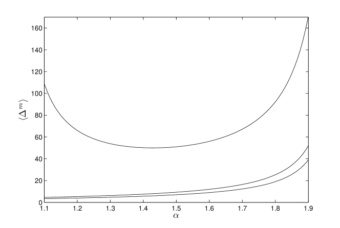
Figure 3: Dependences of the cluster durations $\langle\Delta\rangle$ (47) (bottom curve), $\langle\Delta^{1}\rangle$ (52) (middle curve) and $\langle\Delta^{2}\rangle$ (59) (top curve) as functions of the exponent $\alpha$. The plot corresponds to the critical case $n=1$ with $\kappa=0.25$. Recall that $\langle\Delta^{m}\rangle$ is defined as the mean duration of the clusters that contain at least $m$ aftershocks. In our notations, $\langle\Delta\rangle$ corresponds formally to $\langle\Delta^{0}\rangle$, i.e., it also takes into account the empty clusters for which the noise earthquake does not trigger any aftershock.

In particular, taking into account that

$$\begin{array}[]{c}p(0)=p_{1}(0)=1-n+\kappa,\qquad p(1)=p_{1}(1)=n-\alpha\kappa,\\[2.84526pt] \displaystyle w(\varrho|1)=f_{1}(\varrho)\qquad\Rightarrow\qquad\langle\Delta|j\rangle=1~{},\end{array}$$ (57)

we obtain

$$\langle\Delta^{2}\rangle=\frac{\langle\Delta\rangle-p(1)}{1-p(0)-p(1)}.$$ (58)

Using (57) for $n=1$ and the expression (47) for $\langle\Delta\rangle$, we obtain the mean duration of clusters containing more than one aftershock:

$$\langle\Delta^{2}\rangle=\frac{1-\kappa(2-\alpha)(2-\alpha\kappa)}{\kappa^{2}(\alpha-1)(2-\alpha)}~{}.$$ (59)

The dependences of the cluster durations $\langle\Delta\rangle$ (47), $\langle\Delta^{1}\rangle$ (52) and $\langle\Delta^{2}\rangle$ (59) as functions of the exponent $\alpha$ are shown in figure 3. Note the large jump in mean durations of clusters containing at least two aftershocks compared with clusters containing at least one aftershock.

IV Pdf of recurrence intervals

IV.1 General relations

The knowledge of the exact probability $\text{P}(\tau)$ (16) allows one to calculate exactly the pdf $f(\tau)$ of the random waiting times $\{T_{k}\}$ between subsequent earthquakes. Indeed, a general result of the theory of point processes states that

$$f(\tau)=\langle\tau\rangle\frac{d^{2}\text{P}(\tau)}{d\tau^{2}}~{},$$ (60)

where $\langle\tau\rangle=\text{E}\left[T_{k}\right]$ denotes the mean waiting time between subsequent earthquakes. Therefore, the complementary cumulative distribution function (ccdf) of the random waiting times is equal to

$$\Psi(\tau)=\text{Pr}\left\{T>\tau\right\}=-\langle\tau\rangle\frac{dP(\tau)}{d\tau}~{}.$$ (61)

By normalization, $\Psi(0)\equiv 1$, so that

$$\frac{1}{\langle\tau\rangle}=-\frac{dP(\tau)}{d\tau}\bigg{|}_{\tau=0}~{}.$$ (62)

Using expressions (16), (18) and (28), we have

$$\text{P}(\tau)=e^{-\nu\overline{F}(\tau)-\nu\tau}~{}.$$ (63)

Making explicit $\overline{F}(\tau)$ with expression (31) yields

$$\frac{dP(\tau)}{d\tau}=\nu\frac{1-n\rho(\tau)+\kappa\rho^{\alpha}(\tau)}{1-n+\kappa\rho^{\alpha-1}(\tau)}e^{-\nu\overline{F}(\tau)-\nu\tau}~{}.$$ (64)

Using (62), we have

$$\langle\tau\rangle=\frac{1-n}{\nu}\qquad\Rightarrow\qquad\Psi(\tau)=-\frac{1-n}{\nu}~{}\frac{dP(\tau)}{d\tau}~{},$$ (65)

and finally obtain

$$\Psi(\tau)=(1-n)\frac{1-n\rho(\tau)+\kappa\rho^{\alpha}(\tau)}{1-n+\kappa\rho^{\alpha-1}(\tau)}e^{-\nu\overline{F}(\tau)-\nu\tau}~{}.$$ (66)

Differentiating this last expression (66) with respect to $\tau$ yields the pdf $f(\tau)$ of waiting times between successive earthquakes:

$$f(\tau)=\Phi(n,\kappa,\alpha,\rho(\tau),\nu)~{},$$ (67)

where

$$\begin{array}[]{c}\displaystyle\Phi(n,\kappa,\alpha,\rho,\nu)=\\[11.38109pt] \displaystyle\left[\mathcal{A}(n,\kappa,\alpha,\rho)+\nu\cdot\mathcal{B}(n,\kappa,\alpha,\rho)\right]~{}e^{-\nu\left(\overline{F}(n,\kappa,\alpha,\rho)+\tau\right)},\end{array}$$ (68)

and

$$\begin{array}[]{c}\displaystyle\mathcal{A}(n,\kappa,\alpha,\rho)=(1-n)(1-\rho)\times\\[14.22636pt] \displaystyle\frac{n(1-n)+\kappa(\alpha-1+(2n-\alpha)\rho)\rho^{\alpha-2}-\kappa^{2}\rho^{2(\alpha-1)}}{(1-n+\kappa\rho^{\alpha-1})^{2}},\\[14.22636pt] \displaystyle\mathcal{B}(n,\kappa,\alpha,\rho)=(1-n)\left(\frac{1-n\rho+\kappa\rho^{\alpha}}{1-n+\kappa\rho^{\alpha-1}}\right)^{2}~{}.\end{array}$$ (69)

Recall that $\rho$ represents $\rho(t)$, which is defined by expression (12).

In the following subsections, we analyze in detail expressions (68) and (69) in order to derive the properties of the pdf $f(\tau)$ (67). Expression (68) suggests that it is natural to decompose the analysis of $f(\tau)$ into two discussions, one centered on the term surviving in the limit $\nu\to 0$ and the other one. The two next subsections analyze these two terms in turn.

IV.2 Case $\nu\to 0$

Taking the limit $\nu\to 0$ amounts to neglecting the occurrence of any noise earthquake within the window $(t,t+\tau)$ of analysis. As shown in the next subsection, this first case already reveals interesting properties of the pdf $f(\tau)$, which remain valid in the general case $\nu>0$.

Putting $\nu=0$ in expression (68) and using (67), we have

$$f(\tau)=\mathcal{A}\left[n,\kappa,\alpha,\rho(\tau)\right]\qquad(\nu=0)~{},$$ (70)

where the function $\mathcal{A}(n,\kappa,\alpha,\rho)$ is given by expression (69).

The main asymptotics of the function $\mathcal{A}(n,\kappa,\alpha,\rho)$ are respectively

• at $\rho\ll 1$:

  $$\mathcal{A}(n,\kappa,\alpha,\rho)\simeq\kappa(1-n)(\alpha-1)~{}\frac{\rho^{\alpha-2}}{(1-n+\kappa\rho^{\alpha-1})^{2}}~{},\qquad\rho\ll 1~{}.$$ (71)

  This regime $\rho\ll 1$ corresponds to $\tau\ll 1$ and thus $\rho\simeq\tau$. Relation (71) thus leads to

  $$f(\tau)\simeq\kappa(1-n)(\alpha-1)~{}\frac{\tau^{\alpha-2}}{(1-n+\kappa\tau^{\alpha-1})^{2}},\qquad\tau\ll 1~{}.$$ (72)

• At $\rho\to 1$:

  $$\mathcal{A}(n,\kappa,\alpha,\rho)\simeq\mathcal{C}(1-\rho)~{},\qquad 1-\rho\ll 1,\qquad\mathcal{C}=\frac{(1-n)(n-\kappa)}{1-n+\kappa}~{}.$$ (73)

  This second asymptotic $\rho\to 1$ corresponds to $1-\rho\ll 1$, which is equivalent to the condition $\tau\gg 1$. Using expression (27), relation (73) leads to

  $$f(\tau)\simeq\mathcal{C}~{}e^{-\tau},\qquad\tau\gg 1.$$ (74)

The denominator of expression (72) determines a new characteristic time scale

$$\tau_{c}=\left(\frac{1-n}{\kappa}\right)^{\frac{1}{\alpha-1}}~{},$$ (75)

from which one can define a critical value for the branching ratio (4)

$$n_{c}=1-\kappa~{},$$ (76)

such that $\tau_{c}>1$ for $n<n_{c}$ and $\tau_{c}<1$ for $n>n_{c}$. We shall refer to the case $n<n_{c}$ as the subcritical regime, while $n_{c}<n<1$ is called the near-critical regime.

For $n<n_{c}$ (subcritical regime), $\tau_{c}\gtrsim 1$, and one may replace the asymptotics (72) by the pure power law:

$$f(\tau)\simeq\kappa~{}\frac{\alpha-1}{1-n}~{}\tau^{-(2-\alpha)}~{},\qquad n\lesssim n_{c}~{}.$$ (77)

In contrast, in the near-critical case $n_{c}<n<1$, expression (72) leads to two power asymptotics:

$$f(\tau)\simeq\begin{cases}\displaystyle\kappa~{}\frac{\alpha-1}{1-n}~{}\tau^{-(2-\alpha)}~{},&\tau\ll\tau_{c}~{},\\[11.38109pt] \displaystyle(1-n)\frac{\alpha-1}{\kappa}~{}\tau^{-\alpha}~{},&\tau_{c}\ll\tau\ll 1~{},\end{cases}\qquad n_{c}<n<1~{}.$$ (78)

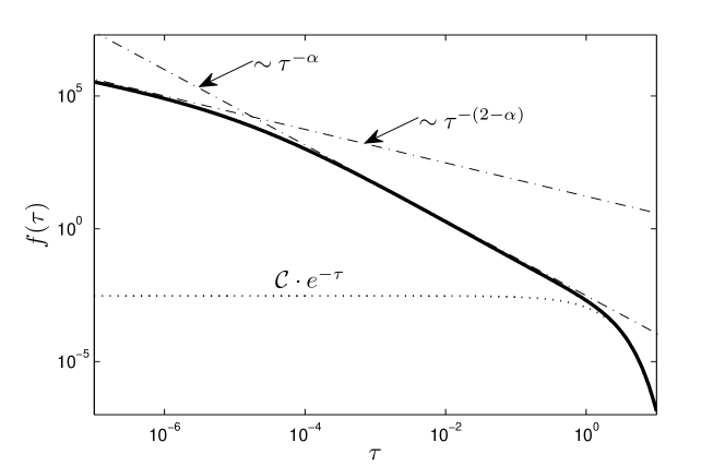
Figure 4: Solid line: Plot of the pdf $f(\tau)$ (70) of waiting times between successive earthquakes for $\nu=0$, $\kappa=0.25$, $\alpha=1.5$ and $n=0.999$. The dotted lines show the power law asymptotics (78) and the exponential asymptotic behavior (74).

Figure 4 shows the pdf $f(\tau)$ (70) of the waiting times between successive earthquakes for $\nu=0$, $\alpha=1.5$, $\kappa=0.25$ ($n_{c}=0.75$), and in the near-critical case $n=0.999$. The two power law asymptotics (78) and the exponential asymptotics (74) for large $\tau$’s are clearly visible. Figure 5 is the same as figure  4, except for the value $n=0.9$. Although, formally, this value belongs also to the near-critical case ($n=0.9>n_{c}=0.75$), the intermediate power law asymptotics $\tau^{-\alpha}$ is barely visible and, for any $\tau\ll 1$, the subcritical power asymptotics $\tau^{-(2-\alpha)}$ dominates at short times.

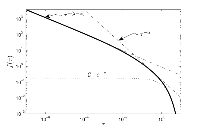
Figure 5: Same as figure 4 except for the value of the branching ratio $n=0.9$.

Figure 6 shows log-log plots of the pdf $f(\tau)$ for $\nu=0$, $\kappa=0.25$, $\alpha=1.5$ and different values of the branching ratio $n$ belonging to the subcritical regime. The subcritical power law asymptotics $\tau^{-(2-\alpha)}$ is dominant and the different pdf’s are similar.

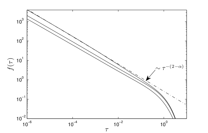
Figure 6: Solid line: Log-log plot of the pdf $f(\tau)$ (70) for $\nu=0$, $\kappa=0.25$, $\alpha=1.5$ and for three $n$ values in the subcritical regime. Top to bottom: $n=0.8;0.6;0.4$. The dotted straight line is the subcritical power law asymptotics (77).

IV.3 General case $\nu\neq 0$

We now take into account the occurrence of noise earthquakes within the window $(t,t+\tau)$ of analysis. The main qualitative difference between this case and the previous one $\nu=0$ is the replacement of the large $\tau$ asymptotics (74) by

$$f(\tau)\simeq(1-n)\left(\frac{n-\kappa}{1-n+\kappa}e^{-\tau}+\nu\right)e^{-\nu(\langle\Delta\rangle+\tau)},\qquad\tau\gg 1~{}.$$ (79)

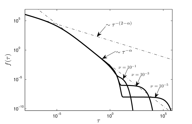
Figure 7: Solid line: Loglog plots of the recurrence times pdf $f(\tau)$ (67) in the case $\kappa=0.25$, $\alpha=1.5$ $n=0.999$ and three subcritical $\nu$ values: $\nu=0.1;10^{-3}$ and $\nu=10^{-5}$. Dotted straight lines are the subcritical and near-critical power asymptotics (74)

The interesting regime of well-defined clusters occurs for $\nu\ll 1$, for which the typical waiting time between noise earthquakes is much larger than the characteristic decay time of the Omori law, which is the typical waiting time between a noise earthquake and its aftershocks. In the interval $1\ll\tau\ll 1\big{/}\nu$, expression (79) reduces to (74) and this exponential decay can be replaced by the plateau

$$f(\tau)\simeq(1-n)\nu~{},\qquad 1\ll\tau\ll 1\big{/}\nu~{}.$$ (80)

For $\tau\gtrsim 1/\nu$, expression (79) simplifies into

$$f(\tau)\simeq(1-n)\nu e^{-\nu\langle\Delta\rangle}~{}e^{-\nu\tau},\qquad\tau\gtrsim 1/\nu~{}.$$ (81)

These different regimes are illustrated in figure 7, which depicts the pdf of waiting times between successive earthquakes for $\kappa=0.25$, $\alpha=1.5$, $\nu=0.999$ and three values of the positive parameter $\nu=10^{-1};10^{-3};10^{-5}$. One can clearly observe the subcritical and near-critical power law asymptotics (78), as well as the plateau (80) joining the exponential asymptotics (74) and (81). The plateau is especially visible for the smallest values $\nu=10^{-3}$ and $\nu=10^{-5}$.

V Conclusion

In this paper, we have studied the impact of the power law form (2) of the distribution of fertilities on the distribution of the recurrence times. In contrast with previous studies, we have considered the simple case where the Omori law is not heavy-tailed but is described by an exponential function. Motivated by real applications, this choice allows us to develop an exact analytical treatment using the formalism of generating probability functions.

Our analysis emphasizes the importance of three time scales controlling the different regimes of the probability density function (pdf) $f(\tau)$ of waiting times between successive earthquakes:

• the characteristic decay time of the exponential Omori law $f_{1}(t)$ (3) describing the occurrence of first generation aftershocks, taken as our time unit,

• the average waiting time $1/\nu$ between two successive “noise earthquakes”, which constitute the exogenous sources of the self-excited processes followed by their aftershocks,

• the characteristic time $\tau_{c}$ defined by expression (75) associated with the self-excited cascades of aftershocks.

In the interesting and relevant regime where earthquake clusters are well defined, namely when the typical waiting time till the first aftershocks (unit time) is smaller than the waiting times $1/\nu$ between noise earthquakes, we have found that the pdf of recurrence times exhibits several intermediate power law asymptotics:

1. For $\tau\ll\tau_{c}$, $f(\tau)\sim\tau^{-(2-\alpha)}$.

2. For $\tau_{c}\ll\tau\ll 1$, $f(\tau)\sim\tau^{-\alpha}$.

3. For $1\ll\tau\ll 1/\nu$, $f(\tau)\simeq(1-n)\nu=const$.

4. For $1/\nu\lesssim\tau$, $f(\tau)\simeq e^{-\nu\langle\Delta\rangle}~{}e^{-\nu\tau}$.

In these formulas, $\alpha$ is the exponent of the power law distribution of fertilities $p_{1}(r)\sim r^{-\alpha-1}$ (2), which is the pdf of the number of first generation aftershocks triggered by a given event of any type. In turn, $n$ stands for the branching ratio defined by equation (4), i.e. the average number of daughters of first generation per mother event, and $\langle\Delta\rangle$ is the mean duration of a cluster that starts with a noise earthquake and ends with its last aftershock over all generation. It is given by expression (43).

Only the first two intermediate asymptotics $f(\tau)\sim\tau^{-(2-\alpha)}$ and $f(\tau)\sim\tau^{-\alpha}$ at short time scales reflect the influence of the power law distribution of fertilities (2), which is revealed by the remarkable effect of the cascade of triggering over the population of aftershocks of many different generations.

Finally, let us stress the differences between the present investigation and our previous work SaiSor2006 ; SaiSor2007 on the same problem. In Refs. SaiSor2006 ; SaiSor2007 , we determined the asymptotic behavior at long times of the distribution of recurrence times, under the approximation that it was sufficient to consider only one aftershock at most per mother event (‘noise earthquake’ in the present terminology). In addition, we considered the standard power law Omori law (1) and not the exponential law (3). By performing a detailed analysis made possible by the use of the exactly tractable exponential Omori law (3), the present paper has thus demonstrated the existence of additional short-time intermediate asymptotics that reveal the distribution of fertilities. This opens the possibility to estimate the exponent $\alpha$ of the distribution of cluster sizes from purely dynamic measures of activity.

Appendix: Statistics of first generation aftershocks

Given the power law (2) for the right tail of the pdf $\{p_{1}(r)\}$ of the number $R_{1}$ of the first generation aftershocks probabilities, we show that the leading relevant terms of the expansion of the GPF $G_{1}(z)$ in powers of $(1-z)$ take the form

$$G_{1}(z)=1-n(1-z)+\kappa(1-z)^{\alpha},\qquad\alpha\in(1,2],$$ (82)

so that the corresponding auxiliary function $Q(y)$ (11) takes the form

$$Q(y)=1-ny+\kappa y^{\alpha}.$$ (83)

They depend on the branching ratio $n$ defined in (4), the exponent $\alpha$ of the power law distribution (2) of the number of first-generation aftershocks. The additional scale parameter $\kappa$ satisfies the following inequalities

$$\begin{cases}0<\alpha\kappa<n,&n\leqslant 1~{},\\ n-1<\alpha\kappa<n,&n>1~{},\end{cases}$$ (84)

which ensure the necessary constraints

$$0\leqslant p_{1}(0)\leqslant 1,\qquad\text{and}\qquad 0\leqslant p_{1}(1)\leqslant 1.$$

Rather than deriving the form (82) from (2), it is more convenient to show that the tail of the pdf $\{p_{1}(r)\}$ whose GPF is given by (82) is the power law (2). Given (82) and the definition linking $G_{1}(z)$ to $p_{1}(r)$, namely $G_{1}(z)=\sum_{j=0}^{+\infty}p_{1}(r)z^{r}$, we obtain

$$p_{1}(0)=1-n+\kappa,\qquad p_{1}(1)=n-\alpha\kappa~{},$$ (85)

and

$$\begin{array}[]{c}\displaystyle p_{1}(r)=\kappa(-1)^{k}\binom{\alpha}{r}=\frac{\kappa(-1)^{r}\Gamma(\alpha+1)}{\Gamma(r+1)\Gamma(\alpha-r+1)},\\[11.38109pt] \displaystyle r\geqslant 2,\qquad\alpha\in(1,2).\end{array}$$ (86)

Using the properties of gamma functions and in particular the well-known equality

$$\Gamma(z)\Gamma(1-z)=\frac{\pi}{\sin\pi z}~{},$$ (87)

we obtain that

$$(-1)^{r}\Gamma(\alpha-r+1)=\frac{\pi}{\Gamma(r-\alpha)\sin[\pi(\alpha-1)]},\qquad\alpha\in(1,2).$$ (88)

Accordingly, expression (86) takes the form

$$p_{1}(r)=c\cdot\frac{\Gamma(r-\alpha)}{\Gamma(r+1)},\qquad c:=\frac{\kappa}{\Gamma(-\alpha)}.$$ (89)

using the asymptotic relation

$$\frac{\Gamma(r+a)}{\Gamma(r+b)}\simeq r^{a-b},\qquad r\to\infty,$$

we finally recover the power law (2).

The case where the exponent $\alpha=2$ in expression (82) of $G_{1}(z)$ requires a special mention. Indeed, this form describes the special situation in which each noise earthquake (and any aftershock as well) can trigger not more than two first generation aftershocks. Accordingly, there are, in general, only three nonzero probabilities

$$p_{1}(0)=1-n+\kappa,\qquad p_{1}(1)=n-2\kappa,\qquad p_{1}(2)=\kappa\qquad(\alpha=2)~{}.$$ (90)

This special situation arises due to the fact that the GPF $G_{1}(z)$ has been truncated beyond the quadratic order $(1-z)^{2}$. It will not be considered further in this paper.

References

- (1) Aït-Sahalia, Y., J. Cacho-Diaz and R.J.A. Laeven, Modeling financial contagion using mutually exciting jump processes, Working Paper 15850, http://www.nber.org/papers/w15850 (2010).
- (2) Azizpour, S., K. Giesecke and G. Schwenkler, Exploring the Sources of Default Clustering, working paper, Stanford University (2010).
- (3) Bak, P., K. Christensen, L. Danon, and T. Scanlon, Unified Scaling Law for Earthquakes, Phys. Rev. Lett. 88, 178501 (2002).
- (4) Barabási, A.-L., The origin of bursts and heavy tails in humans dynamics, Nature 435, 207-211 (2005).
- (5) Bauwens, L. and N. Hautsch, Modelling Financial High Frequency Data Using Point Processes, Handbook of Financial Time Series, Part 6, 953-979, DOI:10.1007/978-3-540-71297-8_41 (2009).
- (6) Chavez-Demoulin, V., A.C. Davison and A.J. McNeil, Estimating value-at-risk: a point process approach, Quantitative Finance, 5 (2), 227-234 (2005).
- (7) Corral, A. (2003), Local distributions and rate fluctuations in a unified scaling law for earthquakes, Phys. Rev. E 68, 035102(R) (2003).
- (8) Corral, A., Universal local versus unified global scaling laws in the statistics of seismicity, Physica A, 340, 590-597 (2004).
- (9) Davidsen, J., S. Stanchits and G. Dresen, Scaling and universality in rock fracture Phys. Rev. Lett. 98, 125502 (2007).
- (10) Errais, E., K. Giesecke and L.R. Goldberg, Affine Point Processes and Portfolio Credit Risk (June 7, 2010). Available at SSRN: http://ssrn.com/abstract=908045.
- (11) Filimonov, V. and D. Sornette, Quantifying reflexivity in financial markets: towards a prediction of flash crashes, Phys. Rev. E 85 (5): 056108 (2012).
- (12) Hawkes, A.G., Point spectra of some mututally exciting point processes. Journal of Royal Statistical Society, series B, 33, 438-443 (1971).
- (13) Hawkes, A.G., Spectra of some mutually exciting point processes with associated variables, In Stochastic Point Processes, ed. P.A.W. Lewis, Wiley, 261-271 (1972).
- (14) Hawkes, A.G. and Adamopoulos, L., Cluster models for earthquakes - regional comparisons, Bull Internat. Stat. Inst. 45, 454-461 (1973).
- (15) Hawkes, A.G. and Oakes D., A cluster representation of a self-exciting process, Journal Apl. Prob. 11, 493-503 (1974).
- (16) Helmstetter, A., Is earthquake triggering driven by small earthquakes? Phys. Res. Lett. 91, 058501 (2003).
- (17) Helmstetter, A. and D. Sornette, Importance of direct and indirect triggered seismicity in the ETAS model of seismicity, Geophys. Res. Lett. 30 (11) doi:10.1029/2003GL017670 (2003).
- (18) Ogata, Y., Statistical models for earthquake occurrence and residual analysis for point processes, J. Am. stat. Assoc. 83, 9-27 (1988).
- (19) Saichev, A., A. Helmstetter and D. Sornette, Anomalous Scaling of Offspring and Generation Numbers in Branching Processes, Pure and Applied Geophysics 162, 1113-1134 (2005).
- (20) Saichev A. and Sornette D., Universal distribution of Interearthquake Times Explained, Physical Review Letters, 97, 078501 (2006).
- (21) Saichev A. and Sornette D., Theory of Earthquake Recurrence Times, Journal of Geophysical Research, 112, B04313-1-26 (2007).
- (22) Saichev, A. and Sornette D., Power law distribution of seismic rates: theory and data analysis, Eur. Phys. J. B 49, 377-401 (2006).
- (23) Salmon, M. and W. W. Tham, Preferred Habitat, Time Deformation and the Yield Curve , working paper (Revised and resubmit - Journal of Financial Markets) (2008).
- (24) Vazquez, A., J. G. Oliveira, Z. Dezso, K. I. Goh, I. Kondor, and A. L. Barabasi, Modeling bursts and heavy tails in human dynamics, Physical Review E 73, 036127 (2006).
- (25) Zaslavsky, G.M. and M.K. Tippett, Connection between recurrence-time statistics and anomalous transport, Phys. Rev. Lett. 67, 3251-3254 (1991).