Synchronization Probability in Large Random Networks
Abstract
In a generalized framework, where multi-state and inter-state linkages are allowed, we derive a sufficient condition for the stability of synchronization in a network of chaotic attractors. This condition explicitly relates the network structure and the local and coupling dynamics to synchronization stability. For large Erdös-Rényi networks, the obtained condition is translated into a lower bound on the probability of stability of synchrony. Our results show that the probability of stability quickly increases as the randomness crosses a threshold which for large networks is inversely proportional to the network size.
I introduction
The synchronization of complex dynamical systems is one of the most intriguing problems and has roots in physics, biology, and engineering Arenas08 . The problem of synchronization in a network of interacting nodes was first brought to attention by Wiener Wiener48 and later pursued by Winfree, who modeled biological oscillators as phase oscillators, neglecting the amplitude Ariaratnam01 Winfree67 .
Following Winfree’s pioneering work, there has been considerable effort to study the structural and dynamical effects of the network and its nodes on the state of synchrony. One important problem encountered in these studies is the possibility of separating the global (network) and local (node) characteristics to allow a general assessment on stability of the synchronous state. In the seminal work by Pecora and Carroll Pecora98 , this issue was addressed by introducing the concept of master stability equation. This equation provides a condition on stability of the network, known as master stability condition (MSC). The MSC also leads to useful bounds on structural properties of the network such as eigenvalues of the Laplacian matrix of the network Newman10 Pecora98 . Following this important result, most of the focus has been directed toward interpreting the bounds on eigenvalues of the Laplacian matrix of the network implied by the MSC as bounds on the degrees of nodes in the network. In Nishikawa03 and Wang02 , the effect of heterogeneity and smallness of the network on synchronization stability have been investigated and it has been shown that if the network is more homogeneous the stability of synchrony is easier to achieve. Though most efforts have focused on the unweighted and undirected graphs, Motter07 and Zhou06 have investigated the master stability equation in directed and weighted structures, respectively.
Since the synchronization manifold can be considered as a fixed point of a reduced (induced) space, the vast majority of the existing literature on the synchronization in the networks considers the largest traversal Lyapunov exponent as a measure of stability of the synchronization. Of course, as noted in Pecora98 , the negativity of Lyapunov exponents is not a necessary nor a sufficient condition on the stability of manifold itself and it does not stop the manifold from bubbling and bursting Daleckii74 Leonov07 .
In this paper, we use an alternative master stability equation derived from Lyapunov direct method to obtain a condition on the stability of the whole network, based on the eigenvalues of symmetric part of local and coupling dynamics. Since this condition encompasses the Lyapunov spectrum, it is a sufficient condition on the stability Daleckii74 . Furthermore, we generalize the conventional setup where the linkage matrices are diagonal (often with binary components) to the case of an arbitrary linkage matrix, allowing multi-state and cross-state linkages, possibly with different strengths, which is now receiving more attention Martins01 Medvedev10 .
We then use the derived MSC to calculate a lower bound on the probability of stability for large Erdös-Rényi networks. We relate the condition of stability to dynamical characteristics of individual nodes and their coupling and structural properties of the Erdös-Rényi networks, namely, network size and randomness parameter.
II System Model
Consider a network of identical nodes with identical coupling dynamics
| (1) |
where denotes the state vector of node , and and denote the node and coupling dynamics, respectively. is the Laplacian matrix of the network. Since L has zero row-sum, this network has a synchronization state, , which is the solution of local state equation, , and . This equation also defines the synchronization manifold. To maintain the synchrony throughout the network, all should converge to a synchronous state, . This means that all the modes traverse to the synchronization manifold should be damped out Pecora98 . Denote the deviation of the state of each node from the synchronous state by . If are small, (1) can be linearized around as
| (2) |
where F and H are Jacobian matrices of and around , respectively. Note that in general, is time dependent and so are the Jacobians. Here, for brevity of the presentation, we have dropped the explicit dependence of F and H on (and therefore on time) from our notation. Combining (2) for all i, we obtain the unified dynamical equation of the whole network as
| (3) |
where is the identity matrix of size , denotes the Kronecker product, and is the error vector with respect to , where . Superscript denotes the transpose operator.
In the rest of the paper, we assume that the network is undirected, and therefore its Laplacian matrix is symmetric, i.e., for all .
III Network stability condition
The network synchronization is exponentially stable around , if is exponentially stable. Due to zero row sum property of L, its smallest eigenvalue, , is zero Mohar91 . The mode for in (3) represents the variation parallel to manifold and hence should be omitted in the study of stability for traversal exponents Pecora98 . Furthermore, multiplicity of zero in the set of network eigenvalues is one, if and only if the the graph is connected Mohar91 . The remaining modes in (3) are traverse to the synchronization manifold and they decay exponentially if and only if the corresponding modes of the system governed by are exponentially stable.
Now, considering the system (3), the norm of e can be bounded by (Leonov07 Thms. 1 and 2)
for all and some . Here denotes the largest eigenvalue of the argument. We note that if for all , the exponent approaches negative infinity as approaches infinity and the system is stable. Thus, a sufficient condition on stability is
here denotes negative definiteness of a matrix. This condition guaranties damping of traverse modes and can be used as stability criteria in the study of dynamical systems Pecora98 .
Since can be written in block Jordan form, the equivalent sufficient condition on asymptotic stability for (3) yields
| (4) |
for . Hence, is exponentially stable if and only if is stable for all , where is the th largest eigenvalue of L (see appendix for propf). The condition in (4) requires the largest eigenvalue of symmetric part of to be strictly negative, and not approaching zero from below. Here we have used the assumption that L is symmetric. Thus, are real and non-negative111In the case of directed network, is replaced with , where superscripts and denote Hermitian and complex conjugate operators, respectively.. In the case of complex F and H, Hermitian operator replaces the transpose operator.
Now we can use Weyl’s inequalities to further explore (4). The Weyl inequalities provide upper and lower bounds on the eigenvalues of sum of Hermitian matrices. Assume that and are Hermitian matrices, and , then Weyl’s inequalities state that (So94 Thm. 1.3)
| (5) |
and
| (6) |
where denotes the th largest eigenvalue of the argument. Utilizing (5) with and (6) with yields
| (7) |
and
| (8) |
for . Now, since and are Hermitian, we can use (7) and (8) to bound from both sides:
| (9) |
and
| (10) |
for .
To obtain a sufficient condition on stability we now force the upper bound in (9), to be negative
| (11) |
for and some . Since maybe positive or negative, the second term in (11) reduces to . Thus, a sufficient condition on stability is
| (12) |
for some , where .
We can also derive a necessary condition for (4) by forcing the lower bound in (10) to be negative, or
| (13) |
Let be the index of smallest positive eigenvalue of . Then (13) reduces to
| (14) |
where
and
In the case that , if then the condition (4) is not satisfied, and if , the corresponding condition can be eliminated.
We note that, (14) is a necessary condition on (4), which itself is a sufficient condition on stability. Therefore (14) does not reveal anything about the stability of the network. However, since (12) and (14) sandwich (4), (14) provides some information regarding how close (4) and (12) are.
Having developed the bounds on condition (4), namely (12) and (14), we now proceed to relate them to the degree properties of the network. To do this, we employ following inequalities known for symmetric Laplacian matrices Mohar91
and
where and denote the maximum and minimum node degrees, respectively. Using these, and (12), the stability condition can be also expressed as
where
and
| (15) |
Similarly, necessary conditions for (4) become
where
and,
From (12) one can draw the conclusion that in the network with low algebraic connectivity, , synchronization is difficult to achieve. This behavior is caused by the fact that the coupling is not strong enough to push/pull the oscillators to synchronous state. And from (15) we can see the other case of non-synchronization behavior occurs when (some) nodes have too many connections (condition on ). This phenomenon is known as synchronization quenching, where the coupling is so strong that eliminates the self-drive of (some of) the oscillators and consequently, the network cannot achieve synchrony Osipov97 .
IV Probability of stability for Erdös-Rényi networks
In the following, we investigate probability of stability of Erdös-Rényi networks Bollobas01 . For large Erdös-Rényi networks with randomness parameter , we can use (12) and (14) to calculate the lower and upper bounds on the probability of (4) being satisfied. We recall that (12) provides a lower bound on the probability of stability, whereas (14) describes the closeness of this lower bound and the probability of (4).
Since eigenvalues of any large randomly generated symmetric matrix follows the Wigner’s semi-circular distribution Wigner58 , we can approximate the distribution of eigenvalues of Laplacian for an Erdös-Rényi network. By definition where A is the adjacency matrix of the network, and is the degree sequence of the nodes. Also in large Erdös-Rényi network, we can approximate by , the average degree of the network Bollobas01 . Hence, . Thus the eigenvalues of L have (approximately) the following distribution Wigner58
where
The order statistics and have densities
and
where
Now, we can evaluate the probability of occurrence of each conditions given in (12) and (14). The lower bound on the probability of stability attained from Wigner’s approximation for (12) is
| (16) |
Similarly, an upper bound on the probability of (4) being satisfied can be derived by applying Wigner’s approximation to (14)
| (17) |
Since these probabilities have relatively sharp roll-offs as a function of (see numerical results), we can use randomness values, , which yield and , to study the synchrony trends as network parameters change. From (16) and (17), we have
and
Thus, the value of randomness, p, required to have stable synchronous state decreases as .
V Numerical Results
For a numerical example, we consider a network of Rössler oscillators (with parameters , , and ) Sorrentino08 coupled through all of their states. This set of parameters results in a coherent chaotic oscillation, since Osipov97 . Therefore, the Jacobian of the oscillator can be computed as
We also assume
where , is the coupling strength.
With this setting we calculate our results on the probability of stability of the network for different values of , , and . To this end, we have considered trajectories starting from initial point where ’s are selected uniformly from interval and all the corresponding eigenvalues are calculated over average of cycles of initiated trajectories.
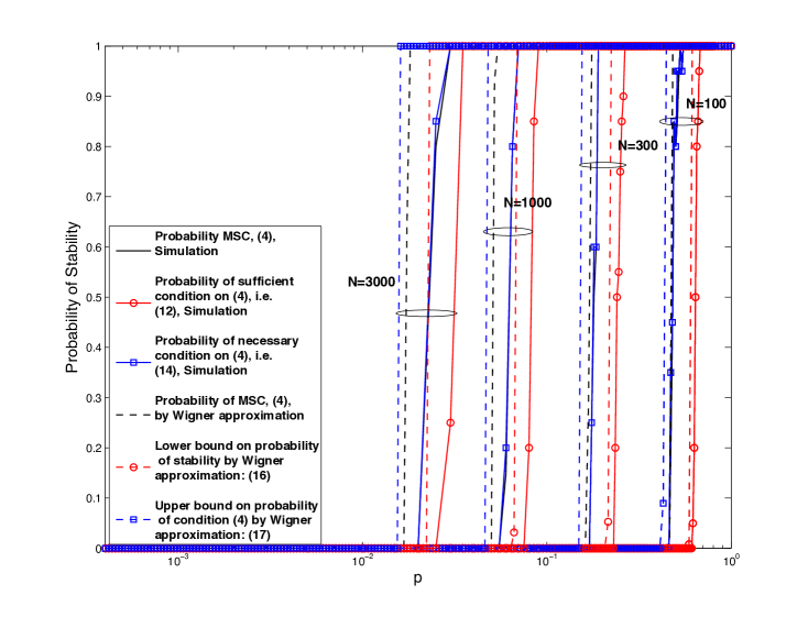
Fig. 1 shows the probability of the stability of the network as a function of network randomness, p, for different network size, N, and with coupling strength . As it can be seen, probabilities of (12) and (14) are close to that of (4). Moreover, we observe that the approximated probabilities provided by the Wigner’s distribution of eigenvalues of the network are also reasonably close.
As Fig. 1 shows for positive definite in a large network if the average degree, , is above some threshold, , (in this example approximately ) the network becomes stable. Note that in this particular numerical example, due to positive definiteness of , only the transition from asynchrony to synchrony is observed.
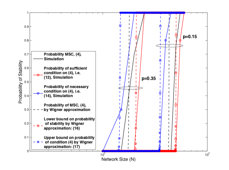
The behavior of the network in the sense of its stability versus network size for several values of is shown in Fig. 2. Once again we observe that the probability of stability suddenly increases as crosses the threshold above.
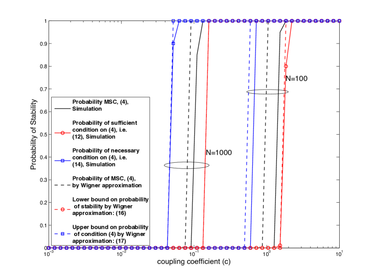
Fig. 3 shows that the stability of the network grows as the network size and coupling factor increase. Of course this is due to our choice of coupling dynamics which is positive definite and by increasing coupling strength, it provides stronger negative feedback to stabilize the network.
VI Conclusion
In conclusion, considering an alternative master stability condition, we have derived a sufficient condition of stability which is a function of the eigenvalues of network structure and symmetric parts of linearized local and coupling dynamics. Our condition relates the largest eigenvalues of the symmetric coupling and the symmetric local dynamics to stability conditions of the networks. For Erdös-Rényi network we have calculated a lower bound on the probability of stability. Then we have proceeded to calculated associated threshold value of randomness where the system starts to become stable as increases beyond this threshold. The reason for this phenomenon is that below the certain threshold, all or some of the nodes cannot achieve sufficient information exchange. As a result, those nodes cannot synchronize themselves with the rest of the network.
Appendix A Appendix: stability of
Since Lis real and symmetric, it is unitarily and orthogonally diagonalizable (Ch. 5.4. [15]). That is, , where is unitary and is diagonal Laub05 . Define . Since e are mapped to by a non-singular linear transformation ( is unitary), their stabilities are equivalent. We have
| (18) |
using the properties of the Kronecker product we have
The matrix is block diagonal. Thus the resultant diagonal block matrix has as its diagonal blocks. In other words, stability of is equivalent to stability of for .
References
- (1) A. Arenas, A. Diaz-Guilera, J.n Kurths, Y. Moreno and C. Zhou, “Synchronization in complex networks”, Elsevier, Physics Reports, Vol. 469, NO. 3, pp. 93–153, 2008.
- (2) J. T. Ariaratnam and S. H. Strogatz, “Phase Diagram for the Winfree Model of Coupled Nonlinear Oscillators”, Phys. Rev. Lett., 2001, Vol. 86, NO. 19, pp. 4278–4281.
- (3) G. A. Leonov and N. V. Kuznetsov, “Time-Varying Linearization and the Perron Effects”, International Journal of Bifurcation and Chaos, 2007, Vol. 7, NO. 4, pp. 1079–1107
- (4) L. C. Martins and L. G. Brunnet, “Multi-state coupled map lattices”, Physica A: Statistical Mechanics and its Applications, 2001, Vol. 296, NO. 1, pp.119 - 130.
- (5) G. S. Medvedev, “Synchronization of coupled limit cycles”, Journal of Nonlinear Science, Springer, 2011, Vol. 21, NO. 3, pp. 441–464.
- (6) B. Mohar, “Graph Theory, Combinatorics, and Applications”, Wiley, 1991, pp. 871-898.
- (7) A. E. Motter, “Bounding network spectra for network design”, New Journal of Physics, 2007, Vol. 9, NO. 6, p. 182.
- (8) T. Nishikawa, A. E. Motter, Y. C. Lai and F. C. Hoppensteadt, “Heterogeneity in Oscillator Networks: Are Smaller Worlds Easier to Synchronize?” Phys. Rev. Lett., 2003, Vol. 91, NO. 1, pp. 014101-4.
- (9) G. V. Osipov, A. S. Pikovsky, M. G. Rosenblum and J. Kurths, “Phase synchronization effects in a lattice of nonidentical Rössler oscillators”, Phys. Rev. E, 1997, Vol. 55, NO. 3 pp. 2353–2361.
- (10) L. M. Pecora and T. L. Carroll, “Master Stability for Synchronized coupled system”, Physical Review Letters, 1998, Vol. 80, NO. 10, pp. 2109-2112.
- (11) Wasin So, “Commutativity and spectra of Hermitian matrices”, Linear Algebra and its Applications, 1994, Vol. 212, pp.121 - 129.
- (12) F. Sorrentino and E. Ott, “Adaptive Synchronization of Dynamics on Evolving Complex Networks”, Physical Review Letters, 2008, Vol. 100, NO. 11, pp. 114101-4.
- (13) Z. F. Wang and G. Chen, “Synchronization in Small-World Dynamical Networks”, International Journal of Bifurcation and Chaos, 2002, Vol. 12, NO. 1, pp. 187-192.
- (14) E. P. Wigner, “On the Distribution of the Roots of Certain Symmetric Matrices”, The Annals of Mathematics, Mar., 1958, Vol. 67, NO. 2, pp. 325-327.
- (15) A. T. Winfree, “Biological rhythms and the behavior of populations of coupled oscillators”, Journal of Theoretical Biology, 1967, Vol. 16, NO. 1, pp. 15-42.
- (16) C. Zhou, A. E. Motter and J. Kurths, “Universality in the Synchronization of Weighted Random Networks”, Phys. Rev. Lett., 2006, Vol. 96, NO. 3.
- (17) B. Bollobas, “Random Graphs”, Cambridge University Press, 2001.
- (18) J. L. Daleckii and M. G. Krein, “Stability of Solutions of Differential Equations in Banach Space”, American Mathematical Society, 1974, pp. 116–127.
- (19) A. J. Laub, “Matrix Analysis for Scientists and Engineers”, SIAM, 2005, pp. 139-150.
- (20) M. E. J. Newman, “Networks: An Introduction”, Oxford University Press, 2010.
- (21) N. E. Wiener, “Cybernetics: Or Control and Communication in the Animal and the Machine”, John Wiley & Sons, 1948.