Effect of turbulent density-fluctuations on wave-particle interactions and solar flare X-ray spectra

Abstract

Aims. The aim of this paper is to demonstrate the effect of turbulent background density fluctuations on flare-accelerated electron transport in the solar corona.

Methods. Using the quasi-linear approximation, we numerically simulated the propagation of a beam of accelerated electrons from the solar corona to the chromosphere, including the self-consistent response of the inhomogeneous background plasma in the form of Langmuir waves. We calculated the X-ray spectrum from these simulations using the bremsstrahlung cross-section and fitted the footpoint spectrum using the collisional “thick-target” model, a standard approach adopted in observational studies.

Results. We find that the interaction of the Langmuir waves with the background electron density gradient shifts the waves to a higher phase velocity where they then resonate with higher velocity electrons. The consequence is that some of the electrons are shifted to higher energies, producing more high-energy X-rays than expected if the density inhomogeneity is not considered. We find that the level of energy gain is strongly dependent on the initial electron beam density at higher energy and the magnitude of the density gradient in the background plasma. The most significant gains are for steep (soft) spectra that initially had few electrons at higher energies. If the X-ray spectrum of the simulated footpoint emission are fitted with the standard “thick-target” model (as is routinely done with RHESSI observations) some simulation scenarios produce more than an order-of-magnitude overestimate of the number of electrons $>50$keV in the source coronal distribution.

1 Introduction

The unprecedented RHESSI observations of solar flare hard X-rays (HXRs, typically $>20$keV) has forced us to consider mechanisms in addition to the traditional collisional view of coronal electron transport. This standard approach is of an assumed power-law of electrons above a low-energy cut-off that propagate downwards, losing energy through Coulomb collision with the “cold” background plasma (whose energy is considerably lower than that of the electrons in the beam). The electrons will eventually stop once they have reached the higher density chromosphere (the “thick-target”), emitting X-rays via bremsstrahlung and heating the plasma. The “cold thick-target” model CTTM (Brown 1971; Syrovatskii & Shmeleva 1972) has proved popular because it provides a straightforward relationship between the bright X-ray emission from the chromospheric footpoints and the source coronal electron distribution. However, many RHESSI observations are not consistent with the CTTM or produce challenging results (Holman et al. 2011; Kontar et al. 2011), which demonstrates that essential physics is missing from the standard model.

One aspect missing from the CTTM are non-collisional processes such as wave-particle interactions. The self-consistent generation of Langmuir waves by the electron beam is one such process that is thought to be the related to the decimetric radio emission in reverse-slope Type III bursts in some flares (Tarnstrom & Zehntner 1975; Aschwanden et al. 1995; Klein et al. 1997; Aschwanden & Benz 1997). We have previously shown that including Langmuir waves helps in alleviating the discrepancies between the CTTM and RHESSI observations. For instance, the CTTM predicts a “dip” to appear in the flare electron spectrum between the thermal component and just before the turnover in the electron beam spectrum. Observationally this has not been confirmed and we showed that the growth of Langmuir waves flattens the electron spectrum at lower energies, maintaining a negative gradient between the thermal and non-thermal spectral component (Hannah et al. 2009). Another observational challenge is the difference in the HXR spectral indices found between the footpoint and coronal sources, which the CTTM predicts to be $\Delta\gamma=2$, yet RHESSI’s imaging spectroscopy of some flares has found values with $\Delta\gamma>2$ (Emslie et al. 2003; Battaglia & Benz 2007; Saint-Hilaire et al. 2008; Battaglia & Benz 2008; Su et al. 2009). We found that the flattening of the electron distribution as it propagates from the corona to the chromosphere due to the generation of Langmuir waves can produce the observed larger differences (Hannah & Kontar 2011).

Wave-particle interactions can produce some observational features of flares better than the CTTM but the flattening of the electron distribution to lower energies through Langmuir wave growth produces far fainter HXR emission. This means that a higher number of electrons need to be accelerated in the corona for the simulations including wave-particle interactions to produce a similar magnitude of HXRs to the standard collisional approach. Compounding this problem further is that the CTTM itself needs a large number of electrons to be accelerated in the corona, which conflicts with the maximum resupply rate of electrons in the coronal acceleration region in some models.

The Langmuir waves themselves might provide a solution to this problem as they can be scattered or refracted when interacting with an inhomogeneous background plasma (Ryutov 1969), which can result in electron acceleration (e.g. Melrose & Cramer 1989; Kontar 2001a, b; Reid & Kontar 2010) and increased X-ray emission (Kontar et al. 2012). The core idea is that the waves can be shifted to a lower wavenumber (higher phase velocity) by interacting with the density gradient in the background plasma, which then resonates with electrons at higher velocity. Although this can happen in the opposite direction (with the waves shifted to higher wavenumber), the falling power-law electron distribution always means that this effect has the strongest consequences for the re-acceleration of electrons to higher energies. Recently, the role of the non-uniform plasma has been studied for an interplanetary electron beam (Reid & Kontar 2010, 2012) and in the stationary (no spatial evolution) case for solar flares in the corona (Kontar et al. 2012). It was found that this can lead to additional electron acceleration. In these studies different forms of the inhomogeneity in the background plasma were considered, including a Kolmogorov-type power-density spectrum of fluctuations, which imitates the spectra expected from low-frequency MHD-turbulence.

In this paper, we demonstrate the consequences of this self-consistent treatment of electron beam-driven Langmuir waves propagating through an inhomogeneous background plasma. This is simulated using the quasi-linear weak-turbulence approach and is detailed in §2. The resulting electron and spectral wave density distributions for a variety of forms of the input electron beam are shown in §3. The mean electron (deducible from observations) and X-ray spectra are obtained for these simulations and the latter are fitted as if they were observations, using the standard CTTM approach. This allows us to determine the discrepancy between the CTTM-derived and true properties of the source electron distribution in §3.1.

2 Electron beam simulation

Following the previously adopted approach (Hannah et al. 2009; Hannah & Kontar 2011), we simulated a 1D velocity ($v\approx v_{||}\gg v_{\bot}$) electron beam $f(v,x,t)$ [electrons cm^-4 s] from the corona to the chromosphere, that self-consistently drives Langmuir waves (of spectral energy density $W(v,x,t)$ [erg cm^-2]). This weakly turbulent description of quasi-linear relaxation (Vedenov & Velikhov 1963; Drummond & Pines 1964; Ryutov 1969; Hamilton & Petrosian 1987; Kontar 2001a; Hannah et al. 2009) is given by

$$\frac{\partial f}{\partial t}+v\frac{\partial f}{\partial x}=\frac{4\pi^{2}e^{2}}{m_{\mathrm{e}}^{2}}\frac{\partial}{\partial v}\left(\frac{W}{v}\frac{\partial f}{\partial v}\right)+\gamma_{\mathrm{C_{F}}}\frac{\partial}{\partial v}\left(\frac{f}{v^{2}}+\frac{v_{\mathrm{T}}^{2}}{v^{3}}\frac{\partial f}{\partial v}\right)$$ (1)

$$\frac{\partial W}{\partial t}+\frac{3v_{\mathrm{T}}^{2}}{v}\frac{\partial W}{\partial x}+\frac{v^{2}}{L}\frac{\partial W}{\partial v}=\left(\frac{\pi\omega_{\mathrm{p}}}{n}v^{2}\frac{\partial f}{\partial v}-\gamma_{\mathrm{C_{W}}}-2\gamma_{\mathrm{L}}\right)W+Sf,$$

where $n$ the background plasma density, $m_{\mathrm{e}}$ the electron mass and $\omega_{\mathrm{p}}^{2}=4\pi ne^{2}/m_{\mathrm{e}}$ is the local plasma frequency. The first terms on the right-hand side of Eqs. (1) and (2) describe the quasi-linear interaction, the other terms the Coulomb collisions $\gamma_{\mathrm{C_{F}}}=4\pi e^{4}n\ln{\Lambda}/m_{\mathrm{e}}^{2}$ and $\gamma_{\mathrm{C_{W}}}=\pi e^{4}n\ln{\Lambda}/(m_{\mathrm{e}}^{2}v_{\mathrm{T}}^{3})$ with $\ln{\Lambda}$ the Coulomb logarithm, Landau damping $\gamma_{\mathrm{L}}=\sqrt{\pi/8}\omega_{\mathrm{p}}\left(v/v_{\mathrm{T}}\right)^{3}\exp{(-v^{2}/2v_{\mathrm{T}}^{2})}$, and spontaneous wave emission $S=\omega_{\mathrm{p}}^{3}mv\ln{(v/v_{\mathrm{T}})}/(4\pi n)$. The simulations here feature two changes over the previous work (Hannah et al. 2009; Hannah & Kontar 2011). The first minor change is the inclusion of the diffusion in velocity space due to collisions (final term in the brackets at the end of Eq. (1)). Previously only the drag term was used, which described a “cold” target situation in which the energy in the beam electrons is considerably higher than that of the background thermal distribution. Including the diffusion term allows a more realistic treatment of electrons at energies closer to the thermal background, i.e. a “warm” target. The second, and more substantial, change is the inclusion of a turbulent background plasma and the effect of this density gradient on the plasma waves (third term on the left-hand side of Eq. (2). This is done using the characteristic scale of the plasma inhomogeneity $L^{-1}=(\partial\omega_{\mathrm{p}}/\partial x)\omega_{\mathrm{p}}^{-1}=(\partial n/\partial x)(2n)^{-1}$ as used previously by Kontar (2001a) and Reid & Kontar (2010).

The electron distribution is simulated in the velocity domain from the 1MK background plasma thermal velocity $v_{\mathrm{T}}$ up to $115v_{\mathrm{T}}$ This range extends below the observational capacity of RHESSI (down to about 86eV instead of RHESSI’s 3keV limit), well into the range where the thermal emission will dominate. Although the treatment of the thermal distribution is beyond the scope of this work, the energy range is included to demonstrate the possible effect these lower energy electrons have on the higher energy population.

The initial electron distribution is Gaussian of width $d=2\times 10^{8}$cm and a broken power-law in velocity, which is flat below the break. This break is effectively the low-energy cut-off. We used $v_{\mathrm{C}}\approx 9v_{\mathrm{T}}$ ($E_{\mathrm{C}}=7$keV), and the power-law above it has an index of $2\delta_{\mathrm{b}}$ (hence a spectral index of $\delta_{\mathrm{b}}$ in energy space), i.e.

$$f(v,x,t=0)\propto n_{\mathrm{b}}\exp{\left(-\frac{x^{2}}{d^{2}}\right)}\left\{\begin{array}[]{l l}1&\quad\mbox{ $v_{\mathrm{T}}<v<v_{\mathrm{C}}$}\\ \left(v/v_{\mathrm{C}}\right)^{-2\delta_{\mathrm{b}}}&\quad\mbox{ $v_{\mathrm{C}}\leq v<v_{\mathrm{0}}$},\\ \end{array}\right.$$ (3)

where $v_{\mathrm{0}}=90v_{\mathrm{T}}$ is the maximum initial beam velocity, $n_{\mathrm{b}}=\int_{v_{\mathrm{C}}}f\mathrm{d}v$ is the electron beam density above the break/low-energy cut-off. For the simulations presented in this paper we used a beam density above the break of $n_{\mathrm{b}}=10^{8}$cm^-3. At the start of the simulations this beam was instantaneously injected at a height of 40Mm above the photosphere and was not replenished, with the spatial grid extending from 52Mm down to 0.3Mm.

A finite difference method (Kontar 2001c) is used to solve Eqs. (1) and (2), and the code is modular which makes it easy to consider the effects of the different processes. We consider three distinct simulation setups within this paper, namely:

• B: beam-only: We only consider the propagation of the electron distribution subject to Coulomb collisions with the background plasma, similar to the CTTM. Specifically, we only solve Eq. (1), ignoring the quasi-linear term (first term on the right-hand side).

• BW: Beam and waves: We consider the propagation of the electron distribution and the self-consistent driving of Langmuir waves but without the plasma inhomogeneity term. This is solving both Eqs. (1) and (2) but without the last term on the left-hand side of Eq. (2), i.e. ignoring $L^{-1}$.

• BWI: Beam, waves and inhomogeneity: We consider the propagation of the electron distribution, the self-consistent driving of Langmuir waves, and the wave interaction with the inhomogeneous background plasma. This is the full solution to both Eqs. (1) and (2).

These three different simulation setups allow us to investigate electron transport due to collisions (B, akin to the CTTM), collisions and wave-particle interactions (BW), and collisions, wave-particle interactions and the plasma inhomogeneities (BWI).

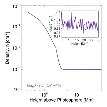
Figure 1: Background plasma density profile $n$. The inset view is of a zoomed portion of the density profile, showing that the density fluctuations (1000 of them with wavelengths between $10^{3}\leq\lambda_{i}\leq 10^{6}$ cm and amplitude of 1%) have been added to the background profile.

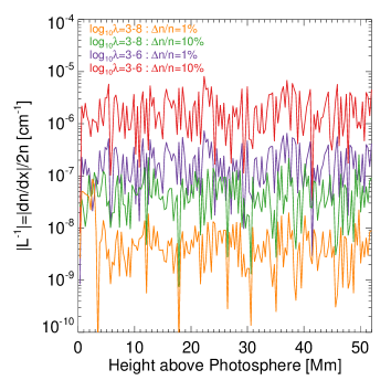
Figure 2: Magnitude of the characteristic scale of the plasma inhomogeneity $L^{-1}$ as a function of height above the photosphere. It is shown for two different wavelength ranges, $10^{3}\leq\lambda_{i}\leq 10^{6}$ cm and $10^{3}\leq\lambda_{i}\leq 10^{8}$ cm, using amplitudes of 1% and 10%.

2.1 Background density fluctuations

The main component of the background density $n_{0}$ is constant in the corona ($10^{10}$cm^-3) and sharply rises through the transition region and chromosphere (below 3Mm). It is shown in Figure 1 and was used previously in Hannah & Kontar (2011). The additional components presented in this paper are the density fluctuations, which are drawn from a turbulent Kolmogorov-type $\beta=5/3$ power density spectrum, i.e.

$$n=n_{0}\left[1+C\sum_{i=1}^{N}\lambda_{i}^{\beta/2}\sin\left(\frac{2\pi x}{\lambda_{i}}+\phi_{i}\right)\right],$$ (4)

where $\lambda_{i}$ are the wavelengths of the density fluctuations, and $C$ is a normalisation constant used to control their amplitude via $\langle\Delta n\rangle/\langle n\rangle=(C^{2}\sum_{i}^{N}\lambda_{i}^{\beta}/2)^{1/2}$, as implemented in Reid & Kontar (2010). Here $N=1000$ fluctuations are added to the background density profile with random phases $\phi_{i}$ between $0$ and $2\pi$ and wavelengths of either $10^{3}\leq\lambda_{i}\leq 10^{6}$ cm and $10^{3}\leq\lambda_{i}\leq 10^{8}$cm chosen randomly in logarithmic space. We investigated two wavelength ranges. One extends to the Mm range, though in both cases it is smaller than the whole simulation region, choosing $C$ to achieve amplitudes of either 1% or 10%. The inset plot in Figure 1 shows the fluctuations for the $10^{3}\leq\lambda_{i}\leq 10^{6}$ cm and 1% case, which are also present in the main plot. The most important aspect of the fluctuations is not the wavelength range or amplitude used, but the resulting magnitude of the density gradient, which influences the waves via the characteristic scale of the plasma inhomogeneity $L=2n(\partial n/\partial x)^{-1}$ in Eq. (2). To calculate this the density gradient of the fluctuations has to be analytically found so that they are accurately included, i.e.

$$\frac{\partial n}{\partial x}=\frac{\partial n_{0}}{\partial x}+C\sum_{i=1}^{N} \frac{\partial n_{0}}{\partial x}\lambda_{i}^{\beta/2} \sin\left(\frac{2\pi x}{\lambda_{i}}+\phi_{i}\right)$$ (5)

$$+2n_{0}\pi\lambda_{i}^{\beta/2-1}\cos\left(\frac{2\pi x}{\lambda_{i}}+\phi_{i}\right).$$

The resulting $L$ for the four different configurations of the fluctuations is shown in Figure 2.

2.2 Simulated X-ray and mean electron spectrum

From these simulations we can compute the X-ray spectrum $I(\epsilon)$ and the mean electron flux spectrum $\langle nVF(E)\rangle$, deducible from the observed X-ray spectrum. For the X-ray spectrum $I(\epsilon)$ we used

$$I(\epsilon)=\frac{A}{4\pi R^{2}}\sum_{E}\sum_{x}\sum_{t}\left[n(x)\frac{f(v,x,t)}{m_{\mathrm{e}}}Q(\epsilon,E)\right]dEdx,dt$$ (6)

where $A$ is the area of the emitting plasma (which we took to be the square of the full width at half-maximum of the Gaussian spatial distribution, i.e. $8(\ln{2}d^{2})$), and $Q(\epsilon,E)$ is the bremsstrahlung cross-section (Koch & Motz 1959; Haug 1997). We calculated the mean electron flux spectrum $\langle nVF(E)\rangle$, which is deducible from the X-ray spectrum (e.g. Brown et al. 2006) by

$$\langle nVF(E)\rangle=\frac{A}{4\pi R^{2}}\sum_{x}\sum_{t}\left[n(x)\frac{f(v,x,t)}{m_{\mathrm{e}}}\right]dxdt,$$ (7)

where $F(E)\mathrm{d}E=vf(v)\mathrm{d}v$ is the electron flux spectrum as a function of energy, not velocity. Most of the spectra shown in §3 are summed over the whole simulation, but for the X-ray footpoint spectrum (§3.1) the summation is over $0.3\leq x\leq 3$Mm.

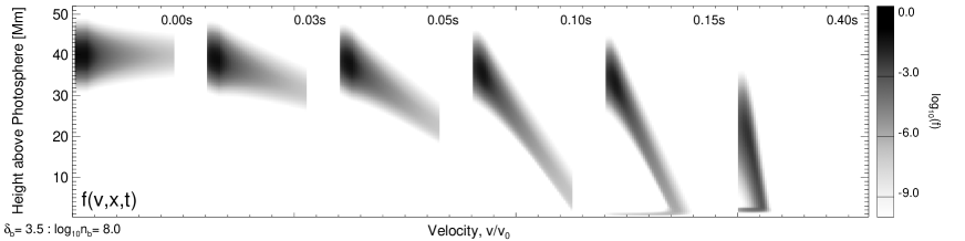
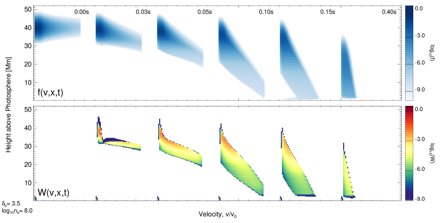
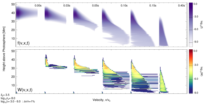
Figure 3: Evolution of the electron $f(v,x,t)$ and wave spectral energy distributions $W(v,x,t)$, with time increasing left to right, for different simulation setups (top to bottom) but all with $\delta_{\mathrm{b}}=3.5$ and $n_{b}=10^{8}$cm^-3. (Top) Electron distribution for the beam-only B simulation. (Middle) Electron distribution and wave spectral energy distribution for the beam and waves BW simulation. (Bottom) Electron distribution and wave spectral energy distribution for the beam, waves and inhomogeneity BWI simulation.

3 Simulation results

Results from one configuration of the three simulation setups is shown in Figure 3, all using an initial beam of $\delta_{\mathrm{b}}=3.5$ and background density fluctuations of $10^{3}\leq\lambda_{i}\leq 10^{6}$ and $\Delta n/n=1\%$. Shown here are the electron $f(v,x,t)$ and wave spectral energy distributions $W(v,x,t)$, in terms of velocity-vs-distance travelled in each frame with time increasing from left to right. The first two configurations, beam-only (B, top panel) and beam and waves (BW, middle panels), show similar results to those that we have previously published (Hannah et al. 2009). Here we are using a higher beam density, however we have a flat (instead of no) electron distribution below $E_{\mathrm{C}}$, and there are density fluctuations in the background plasma. In the beam-only case we see that the fastest electrons reach the lower atmosphere first, quickly lose energy to the high-density background plasma and leave the simulation grid. The bulk of the electron distribution takes longer to lose energy through Coulomb collisions with the background plasma. After 1 second in simulation time the electron distribution is no longer present. When the wave-particle interactions are included (BW, middle panel of Figure 3), the electron distribution immediately flattens/widens in velocity space, with electrons shifted to lower energies. After $t=0.03$s two components of Langmuir waves have developed: one at lower energies through the spontaneous emission, the $Sf$ term in Eq. (2) and another across a wide range of velocities through the propagation of the fastest electrons away from the bulk of the distribution, the $\partial f/\partial x$ term in Eq. (2).

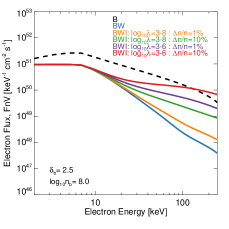
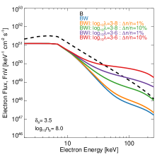
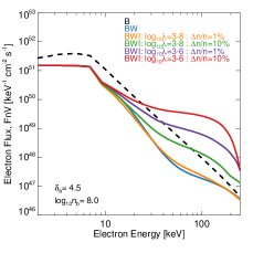
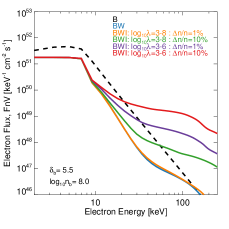
Figure 4: Mean electron flux spectrum (spatially integrated and time averaged) for initial electron beams of power-law index $\delta_{\mathrm{b}}=2.5,3.5,4.5,$ and $5.5$ (increasing left to right). The different colour lines indicate the different simulation setups : B (black dashed), BW (blue), and BWI (orange, green,purple, and red). In the last case two different wavelength ranges are used ($10^{3}\leq\lambda_{i}\leq 10^{6}$ cm and $10^{3}\leq\lambda_{i}\leq 10^{8}$ cm) with fluctuations of the amplitudes of 1% and 10%.

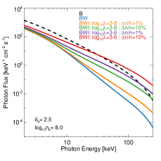
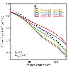
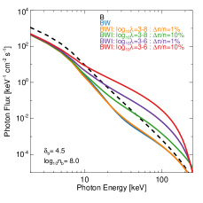
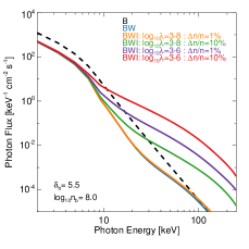
Figure 5: X-ray spectrum (spatially integrated and time averaged) for initial electron beams of power-law index $\delta_{\mathrm{b}}=2.5,3.5,4.5,$ and $5.5$ (increasing left to right). The different colour lines indicate the different simulation setups : B (black dashed), BW (blue), and BWI (orange, green,purple, and red). In the last case two different wavelength ranges are used ($10^{3}\leq\lambda_{i}\leq 10^{6}$ cm and $10^{3}\leq\lambda_{i}\leq 10^{8}$ cm) with fluctuations of the amplitudes of 1% and 10%.

The result that these simulations produce similar results to our previous work confirms that the density fluctuations only play a role once the inhomogeneity term $L$ term is included in Eq. (2), which is shown in the bottom panels of Figure (3). The BWI shows a dramatic change over the other simulations, with streaks appearing in the wave spectral density plots because the waves shift to lower and higher phase velocity (or higher and lower wavenumber). The effect on the electron distribution is to pull it out in clumps across the velocity-space, which is most evident in the $t=0.10$s frame. The leading edge of the electron distribution is clearly pushed out to higher velocities compared to the other setups, i.e. at times $t=0.10,0.15$s the frames of the electron distributions of the B (black) and BW (blue) setups do not extend to energies as high as the BWI (purple) setup in Figure 3.

The change in energy is most evident when the spatially-integrated mean electron spectra $\langle nVF(E)\rangle$ are calculated for the simulations, as shown in Figure 4. Here all configurations of the simulations are shown, indicated by different coloured lines, and the panels show the spectral indices of the initial distribution $\delta_{\mathrm{b}}=2.5,3.5,4.5,$ and $5.5$ increasing from left to right. The mean electron spectrum of the simulations shown in Figure 3 are shown in the second plot in Figure 4, the same colours are used for the electron distributions in each different setup. For the hardest (i.e. flattest, $\delta_{\mathrm{b}}=2.5$, left panel Figure 4) initial spectrum almost all different setups are substantially lower than for the beam-only case. Only the fluctuations with the steepest density gradient (10% and $10^{3}\leq\lambda_{i}\leq 10^{6}$ cm) produce electrons at higher energies than the purely collisional setup, but this only occurs at the highest energies ($>100$keV). With steeper initial spectral indices (larger $\delta_{\mathrm{b}}$) we find that more electrons have been accelerated with even lower levels of density fluctuations, though the inhomogeneity needs to have $L^{-1}\geq 10^{-8}$cm^-1. This may depend on the way the initial distributions were normalised. The same beam density above the low-energy cut-off was used throughout $n_{\mathrm{b}}=\int_{v_{\mathrm{C}}}f\mathrm{d}v$, but for steeper spectra this results in more electrons at energies just above $E_{\mathrm{C}}$. Therefore there is a higher number (about a factor of two from Figure 4) of electrons with about 10 keV with the steeper spectra available to be re-accelerated by the shifted waves. Even for the strongest electron acceleration caused by the density fluctuations, it is only above about 20 keV that there are more electrons than in the beam-only setup. In all simulations where the wave-particle interactions are present, the Langmuir wave generation flattens the spectrum, which reduces the number of low-energy electrons compared to the purely collisional case.

The result of the wave scattering for the HXR spectrum is more complicated since an electron can produce an X-ray below its energy. This is because higher energy electrons can travel farther into the dense regions of the lower solar atmosphere, producing substantially stronger HXR emission. The spatially integrated X-ray spectra for the different simulation setups and configurations are shown in Figure 5. As with the mean electron spectrum, the most significant changes are observed in the simulations with the softest (steepest $\delta_{\mathrm{b}}=5.5$, last panel of Figure 5) initial electron distributions. Here the X-ray emission is up to several orders of magnitudes higher than the beam-only case, whose spectrum is flatter down to 10 keV. This trend continues with the harder initial electron distributions producing flatter X-ray spectrum compared to the purely collisional case. Again with the hardest initial spectrum ($\delta_{\mathrm{b}}=2.5$, first panel Figure 5) only the strongest density fluctuations produce X-ray emission higher than the beam-only case, but this extends to about 30 keV, whereas in the electron spectrum it is only higher $>100$ keV.

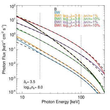
Figure 6: Footpoint X-ray spectrum for an initial electron power-law index of $\delta_{\mathrm{b}}=3.5$ and the different simulation setups (coloured lines). Each is fitted over $20-100$ keV using the f_thick2.pro model, which is indicated by the dashed lines and is similar to the beam-only simulation (B, black line).

3.1 Fitting the footpoint X-ray spectrum

To quantify the effect of the wave-particle interactions and density fluctuations on the X-ray spectrum, we fitted them as if they were actual observations. We specifically fitted the footpoint X-ray spectrum, where in Eq. (6) we summed over the region $0.03\leq x\leq 3$Mm instead of the whole simulation, because in RHESSI observations the flare spectrum is mostly dominated by the footpoint emission from the chromosphere. These spectra were fitted using the implementation of the CTTM in the OSPEX software f_thick2.pro, an optimised version of the routine by G. Holman (usage examples are given in Holman (2003)), available in the SolarSoft X-ray package. We fitted a single power-law as the source spectrum, setting the low-energy cut-off ($E_{\mathrm{C}}=7$keV) and maximum energy to be the same as the initial electron distribution in our simulations. The fitting can be highly sensitive to the low-energy cut-off, so by fixing it to the true simulation value, we avoided this problem, as well as the issue of the missing thermal component at low energies that would be present in real spectral observations. We therefore have two free parameters in our model fit: the total number of electrons $N(>E_{\mathrm{C}})$ and the spectral index $\delta_{\mathrm{TT}}$ of the source distribution. We fitted, by minimizing $\chi^{2}$, the simulated footpoint spectra over 20 to 100 keV, the typical energy range used in RHESSI observations, which also avoids complications of the thermal component at low energies and simulation edge effects at higher energies.

The simulated footpoint spectra (colour lines) and their f_thick2.pro fits (dashed lines) for the initial spectral index $\delta_{\mathrm{b}}=3.5$ are shown in Figure 6 for all simulation setups. In all cases the model fits the simulated spectra very well over the chosen energy range (indicated by the dotted vertical lines). The fitted f_thick2.pro model should be a reasonable match to our simulation B and we obtain $\delta_{\mathrm{TT}}=3.7$ and $N(>E_{\mathrm{C}})=4\times 10^{35}$ electrons. The slight discrepancy between the fitted and true spectral index (3.7 vs 3.5) for the source distribution is because the f_thick2.pro model is steady-state and stationary where as our simulation includes the time and 1D-spatial evolution of an injected (not continuous) electron beam. For the simulations with different initial spectral indices we again find only a small discrepancy to the fitted values, obtaining 2.8, 4.7, and 5.6. In all these B simulations we obtained the total number of electrons in the range of $N(>E_{\mathrm{C}})=3.5-4.7\times 10^{35}$ electrons.

We normalised all fitted results by those found for the B case. They are shown for the spectral indices $\delta_{\mathrm{TT}}$ in Figure 7 and total number of electrons $N(>E_{\mathrm{C}})$ in Figure 8. For the steepest initial distribution ($\delta_{\mathrm{b}}=5.5$) all fitted spectral indices are considerably lower, over 50% lower for the case with the strongest density fluctuations. For this level of turbulence in the background plasma the fitted spectral index is always at least a half of the source index, indicating the consistent flattening and hardening of the spectrum. The only exception to this is for the BW simulation with the hardest source spectrum ($\delta_{\mathrm{b}}=2.5$) where the fitted index is 20% higher. This steeper spectrum is because the loss of higher energy electrons from the initially harder distribution (through the generation of Langmuir waves) dominates over the re-acceleration through the plasma inhomogeneities.

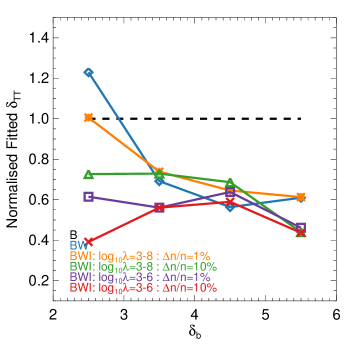
Figure 7: Power-law index of the electron distribution $\delta_{\mathrm{TT}}$ found from fitting f_thick2.pro to the simulated footpoint X-ray spectra as a function of the actual initial power-law index $\delta_{\mathrm{b}}$. The index $\delta_{\mathrm{TT}}$ is normalised by those found from the fit to the beam-only (B, black line) X-ray spectrum.

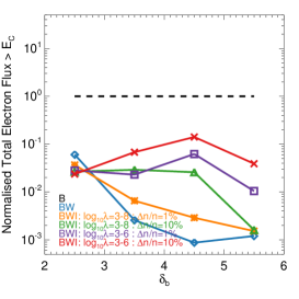
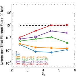
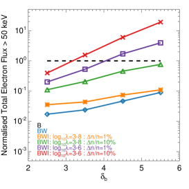
Figure 8: Total number of electrons above $E_{\mathrm{C}}$, 20 keV and 50 keV (left to right) as a function of the power-law index of the initial electron distribution $\delta_{\mathrm{b}}$, obtained from the fitting of f_thick2.pro to the simulated footpoint X-ray spectra. The differently coloured lines indicate the different simulation setups used. The number of electrons are normalised by those from the fit to the beam-only (B, black line) X-ray spectrum.

The total number of electrons in the source distribution inferred from the f_thick2.pro fits is substantially smaller than the true values (first panel in Figure 8). The CTTM interpretation of these spectra is a considerable underestimate (10 to 1 000 times) of the number of electrons in the source distribution. It is clear in the mean electron spectrum (Figure 4) that including the plasma inhomogeneity accelerates electrons to higher energies, which increases the population at energies well above 20 keV. Therefore we also calculated the number of electrons that the f_thick2.pro fit suggests is above 20 and 50 keV in the source distribution, as shown in the middle and last panels of Figure 8. At best, with steep spectra and the strongest fluctuations considered here, the wave scattering can produce a similar number of electrons to those found in the CTTM case for the number of electrons above 20 keV. For the highest energy electrons the situation is considerably better with several simulation setups producing number of electrons $N(>50$keV$)$ similar to or larger than the B case. For the steepest initial spectrum and strongest fluctuations the f_thick2.pro fit overestimates the number of electrons in the source by over an order-of-magnitude, about a factor of 20. However, it is only a limited set of conditions ($L^{-1}\geq 10^{-7}$cm^-1 and $\delta_{\mathrm{b}}\geq 3.5$) that produces more high-energy electrons than f_thick2.pro.

4 Discussion and conclusions

Including Langmuir waves driven by the propagating electron beam causes major changes in the energy of the electrons and produces substantially different X-ray spectra. With no, or low levels $L^{-1}<10^{-8}$cm^-1 of the density fluctuations in the background plasma, the dominant effect is wave-particle interactions that decelerate the electrons, which produces a flatter spectrum and weaker X-ray emission. If these simulated spectra were assumed to be caused by the CTTM the number of electrons in the source distribution would be substantially underestimated . With strong inhomogeneities ($L^{-1}>10^{-7}$cm^-1) in the background plasma there is more re-acceleration of the electrons to higher energies, resulting in harder (flatter, smaller $\delta$) spectra. Interpreting these simulations with the CTTM produces either a similar amount or an overestimate (we found up to $\times 20$) to the number of electrons in the source distribution. Langmuir waves, if generated in solar flares, can produce substantial changes in the flare-accelerated electron distribution. These effects need to be included for a more reliable interpretation of flare HXR spectra.

We found for $L^{-1}\geq 10^{-7}$cm^-1 and $\delta_{\mathrm{b}}\geq 3.5$, the electron re-acceleration becomes sharply pronounced, while the low density gradients are insufficient to shift the energy quickly enough. Indeed, Ratcliffe et al. (2012) showed that the strongest acceleration is achieved when the relaxation time is close to the time scale due to the density inhomogeneity. Because we have a fixed upper limit to the simulation grid $v=115v_{\mathrm{T}}$ the re-acceleration of electrons in the hardest source distributions ($\delta<3.5$) might be lost. We are developing a full relativistic treatment of Eqs. (1) and (2) to study whether the plasma inhomogeneities can have a greater effect for this flatter spectral domain.

Our simulations lack wave-wave interactions. The interaction of Langmuir waves with ion-sound waves has been shown to produce additional electron re-acceleration (Kontar et al. 2012). These simulations had no spatial dependence and work is under way to investigate their role in the 1D simulations presented here. The interaction of Langmuir waves with whistler or kinetic Alfén waves (e.g. Bian et al. 2010) might also produce considerable changes to the electron distribution in flares. The density fluctuations can effectively change the direction of Langmuir waves, and hence depart from the 1D model, which could limit the application of our simulations. Recently Karlický & Kontar (2012) have performed a number of 3D particle-in-cell PIC simulations with initially mono-energetic beams and have shown that during 3D relaxation a population of electrons appear that has velocities exceeding those of the injected electrons. While PIC simulations cannot predict the long-term evolution of these processes as considered here, the number of accelerated electrons at the stage of plateau formation closely matches the numbers estimated using 1D quasilinear equations.