Charge dynamics in an ideal cuprate $Ca_{2-x}Na_{x}CuO_{2}Cl_{2}$: optical conductivity from Yang-Rice-Zhang ansatz

Abstract

We theoretically investigate charge dynamics in weakly coupled $CuO_{2}$ planes of the cuprate $Ca_{2-x}Na_{x}CuO_{2}Cl_{2}$ (CNCOC) using Kubo formula for optical conductivity in the underdoped regime. The spectral function needed in Kubo formula is obtained from an analytical form of electron Green’s function proposed (ansatz) by Yang-Rice-Zhang (YRZ) for the underdoped cuprates based on their previous renormalized mean field theory and on the investigations of weakly coupled Hubbard ladders. Although to an unaided eye the results of the numerical calculation look very similar to that found experimentally in [K. Waku etal. 2004waku ] but a careful examination with extended Drude formalism shows that YRZ ansatz for the calculation of optical conductivity is not sufficient to understand the charge dynamics in $CuO_{2}$ planes of the cuprate CNCOC. More physics is needed especially electromagnetic response from bound charges.

PACS numbers: 74.72.-h; 74.25.Gz; 74.72.Kf; 78.20.Bh

I Introduction

Physical investigations at very small length scale (sub-atomic, atomic etc…) are usually indirect. To expose or uncover the underlying physical reality one has to relay on indirect experimental probes. In simpler situations few experimental probes can give one a consistent physical picture (for example spectral lines of the atomic spectra suggested the discrete energy level structure of atoms). In more complex situations (as for example in high temperature superconductors) one has to deal with several experimental probes. Consistent microscopic physical picture of a material can only be constructed if results of several experimental probes are consistent with each other and comply with one universal picture. And that universal picture is the major deriving force, and at the same time it also puts heavy demands on researchers of understanding an arsenal of complex experimental probes (Fig. 1). In complex situations, understanding reached based solely on few experimental results may not be consistent with other experimental results. One has to be careful. The situation is analogous to the famous story of blind men and an elephant. Each blind man “feels” different part of the elephant and concludes that the elephant is like a snake (for a man who touches the trunk) or like a pillar (for a man who feels the legs ) etc. Only if they positively council (without fighting with each other) they may reach on the “universal” picture of the elephant.

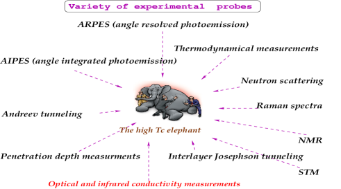
Figure 1: An arsenal of complex experimental probes.

At present, for the cuprate high temperature superconductivity problem we do not have a consistent universal picture for the whole phase diagram consistent with all experimental probes (in any way comparable to the description of ordinary superconductivity by Bardeen, Cooper, and Schrieffer). But there are marvelous attemptsander1 . Cuprates are complex materials with many anomalous properties–not only unconventional superconductivity but also unconventional normal state response. Some of the anomalous properties are as follows. D.C. resistivity of hole doped cuprates just above the optimal doping is linear in temperature $T$ (reminder: for a good metal obeying Fermi Liquid Theory (FLT), $\rho\sim T^{2}$, and $\rho\sim T^{5}$ if phonons also contribute at $T$ ($T<<T_{Debye}$)). Away from optimal doping resistivity shows a very complex behaviourdagotto , and electron doped compounds do not show this linear in temperature behaviour of resistivity! Hall coefficient is temperature dependent (for a good FLT metal it should be temperature independent). For cuprates, Drude scattering rate turns out to be frequency and temperature dependent (for a good FLT metal it is constant (again if phonons do not contribute in the temperature regime of interest)). In the “normal” state above optimal doping real optical conductivity shows $\sim\frac{1}{\omega}$ behaviour (in a good FLT metal it is $\sim\frac{1}{\omega^{2}}$ Drude behaviour). NMR relaxation rate shows substantial deviations from linear in temperature behaviour ($T$-linear Korringa type). High $T_{c}$ cuprates has smaller coherence length (roughly the size of the cooper pair) as compared to conventional (in accord with BCS theory) superconductors. The cooper pair size turns out to be smaller than mean carrier-carrier separation, thus mean-field type approximations in cuprate problem are questionable. There are many other anomalous properties without proper understandingunder . Cuprates show variety of phases with temperature and doping and one of the elusive phases is the pseudogap phase (Fig. 2). There are many views on pseudogap phaseyrzrev , but recently, a broad picture at a phenomenological level of the pseudogap phase is proposed for the cuprate problem. It is contained in Yang-Rice-Zhang (YRZ) ansatzyrzrev ; yrzi . This is based on several inputsyrzrev .

The key element of YRZ’s phenomenological theory is an ansatz for the single electron propagator. This ansatz is the outcome of series of investigations of the proposers over several decades and is primarily based on their renormalized mean field theoryrmft and on the investigations of weakly coupled Hubbard laddersladders . YRZ ansatz has been applied successfully to understand several anomalous properties of the pseudogap phaseyrzrev . This has been applied with success to the interpretation of ARPES (angle resolved photoemission) experiments on CNCOCarpes and good agreement is seen between the calculated hole Fermi pocket and experimental datayrzrev . YRZ ansatz also correctly reproduce particle-hope asymmetry seen in experiments of Yang etalyang . This has also been applied to AIPES (angle integrated photoemission) and qualitatively reproduce the key features of the spectrahash ; yrzrev . For STM (scanning tunneling microscopy) spectra of constant quasi-particle energy contours on BSCCOkoh one sees a qualitative agreement with YRZ, although quantitative fits with experimental spectra are not claimedyrzrev . Raman Spectra is quite useful because it probes both the nodal ($B_{2g}$) and anti-nodal ($B_{1g}$) charge dynamicsram . Valenzuela and Basconesbas found that YRZ qualitatively reproduce features seen in the spectratac (in perticluar they deduce two energy scales, nodal and anti-nodal, with opposite dependence on doping, nodal scale decreases with underdoping while the anti-nodal one increases). YRZ has been applied to several other experimental results see for detailyrzrev . In regard to the microscopic picture, one should clearly distinguish between YRZ ansatz and preformed pair picturepre in which particle-hole symmetry is maintained.

Our interest here is in the optical spectra and in the behaviour of optical conductivity in the pseudogap phase– its variation with doping and temperature. Optical conductivity spectra of the cuprates is complex in comparison to that of conventional superconductors. In conventional superconductors the gap is isotropic in momentum and one gets a clear signature of the gap in the spectrum (In fact early pioneering experiments by Tinkham etaltink gave support to the energy gap model of superconductivity on which Bardeen highly relied and later on a very successful theory of electromagnetic response was put forward by Mattis-Bardeenmb ). In Cuprates gap(s) are anisotropic and optical conductivity spectra becomes intricate. Recently, experimentally observed optical spectra of cuprates has been studied using the YRZ theory by Carbotte, Nicol and colleaguescar . Their investigations support the view that YRZ ansatz qualitatively reproduce low energy behaviour of optical conductivity.

Here, in the present investigation, we re-visit this problem. Our results do not bring any good news for the applicability of YRZ ansatz to the low energy optical response of cuprates. We concentrated on a specific compound $Ca_{2-x}Na_{x}CuO_{2}Cl_{2}$ (CNCOC). The results of our numerical calculation appears to be in qualitative agreement with what has been found experimentally inwaku (to an unaided eye the results look very similar to that found experimentally). But a careful examination with extended Drude formalism shows that YRZ ansatz for the calculation of optical conductivity is not sufficient to understand the charge dynamics in $CuO_{2}$ planes of CNCOC. It seems that more physics is needed to fully understand the optical response.

Rest of the paper is organized as follows. In the next subsection (subsection A) essential points of YRZ ansatz and the cuprates are given. In subsection (B) a brief introduction to optical conductivity and Kubo formalism is given. In section II, CNCOC system and experimental results are summarized. The calculation of optical conductivity using YRZ ansatz and comparison with experiment is given in section III. In section IV extended Drude model analysis is presented to point out the inconsistencies. We end with brief conclusion in section V.

Figure 2: Phase diagram of cuprates.

I.1 Essential points of YRZ ansatz and cuprates

The starting point of YRZ ansatz is the reasonably well understood regimes of extreme underdoping and overdoping (Fig. 2). At overdoping one observes full Fermi surface and it disappears at zero doping. As one shifts from overdoping to underdoping in the phase diagram Fermi surface evolves from full Fermi surface to only disconnected arcs (in specific directions in $k$-space) at underdoping to no Fermi surface at zero doping. The key issue is: how can one explain this doping dependent evolution of the Fermi surface using a microscopic model? The major problem is the intermediate regime and YRZ ansatz is an attempt to fill this gap. As is well known, undoped cuprates are Mott insulators (more precisely charge transfer type) and it was pointed out by Phil Anderson very early on that the operational elements in the cuprate superconductivity are the $CuO_{2}$-planes. $Cu$ atoms in $CuO_{2}$ planes are in $d^{9}$ configuration (with one hole in the higher energy anti-bounding $3d_{x^{2}-y^{2}}Cu--2p_{x(y)}$ orbital lying in $CuO_{2}$ plane). The holes localize (immobile) on atomic sites due strong on-site coulomb repulsion. With further hole doping, new holes are created in $CuO_{2}$ planes. These new holes will not be in $Cu$ $d$-orbitals (because of strong Coulomb repulsion) and tend to be in oxygen $p$ orbitals. It was shown by Zhang and Ricezr that if they form singlet pairs with the holes in $Cu$ atoms then they will have lower energy. These singlet pairs are now called Zhang-Rice (ZR) singlets. We are interested in the transport properties of these ZR singlets. This also reduces the cuprate problem from three band to one band problem (although there are debates in the literaturedebates ). The idea is to reduce the problem to its bare essentials. This motivates the famous $t-J$ modelander1 with no double occupancy at the same site (the Hilbert space of the problem will not have any configuration in which any site is doubly occupied–the projected Hilbert space). One can work in unprojected Hilbert space by using the ideas of Renormalized Mean Field Theory (RMFT)ander1 ; yrzrev . This is the first component of YRZ ansatz. The second component is based on the analytical studies by Konik, Rice, Tsvelik, and Ludwigkonik of 2-leg Hubbard ladders and a collection of weakly coupled Hubbard ladders. For weakly coupled 2-leg Hubbard ladders the coherent part of Green’s function turns out to be (treating the inter-ladder coupling in RPA):

$$G(k_{x},k_{y},\omega) = \frac{1}{G_{0}^{-1}(k_{x},\omega)-t_{y}(k_{y})}$$

$$G^{0}(k_{x},\omega) = \frac{1}{\hbar\omega-\epsilon(k_{x})-\frac{\Delta^{2}}{\hbar\omega+\epsilon(k_{x})}}.$$ (1)

Where $t_{y}$ is the transverse inter-ladder hopping. $\epsilon(k_{y})$ and $\Delta$ are the bare band dispersion and quasi-particle gap respectively.

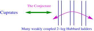
Figure 3: YRZ conjucture: equivalence of many weakly coupled 2-leg Hubbard ladders and $CuO_{2}$ planes in cuprates.

Based on the above two main elements, here is the key postulate: continuous crossover from the weak to strong interaction limit. The coherent part of YRZ Green’s function for the pseudogap state of cuprates is postulated to be:

$$G^{YRZ}(k,\omega) = \frac{g_{t}(x)}{\hbar\omega-\epsilon(k)-\Sigma_{pg}(k,\omega)},$$

$$\Sigma_{pg}(k,\omega) = \frac{|\Delta_{pg}(k)|^{2}}{\hbar\omega+\epsilon_{0}(k)}.$$ (2)

This is essentially based on intuition (Fig. 3). The dressed band dispersion $\epsilon(k)$ contains the renormalization factors of RMFT. Details of bare band and renormalized band dispersions are given in the next section.

I.2 Optical Conductivity

Optical conductivity is the linear response function of an external A. C. electric field. In a rough classical picture the charge carriers oscillate back-and-forth under the influence of an external A.C. electric field (neglecting the weaker ($\frac{1}{c}$th) magnitude magnetic field effects). During this back-and-forth motion they scatter by impurities and phonons causing the dissipation of energy (Joule heating). In the linear response regime induced current density $\bf{J}(\bf{r},\omega)$ is related to the applied electric field $\bf{E}(\bf{r^{\prime}},\omega)$ by

$$\bf{J}(\bf{r},\omega)=\int\sigma(\bf{r},\bf{r^{\prime}};\omega)\bf{E}(\bf{r^{\prime}},\omega)d\bf{r^{\prime}}.$$

If we are not in the anomalous skin effect regime (i.e., electric field does not vary substantially on the length scale of the mean-free-path of charge carriers) then $\sigma(\bf{r},\bf{r^{\prime}};\omega)=\sigma(\bf{r};\omega)\delta(\bf{r}-\bf{r^{\prime}})$ and

$$\bf{J}(\bf{r},\omega)=\sigma(\bf{r};\omega)\bf{E}(\bf{r},\omega).$$

And further if the material is homogeneous:

$$\bf{J}(\bf{r},\omega)=\sigma(\omega)\bf{E}(\bf{r},\omega).$$

The optical conductivity (“Optical”, if $\omega$ is in optical frequency range) $\sigma(\omega)$ can be calculated by using quantum mechanical expression for current density $J=\frac{\hbar}{2mi}(\psi^{\ast}\nabla\psi-\psi\nabla\psi^{\ast})$ and it can be shown that

$$\sigma(\omega,T)=\frac{2\pi e^{2}}{\hbar V}\sum_{k_{x},k_{y},k_{z}}v_{o,x}^{2}(k_{x},k_{y})\times$$ (3)

$$\int_{-\infty}^{+\infty}dy\frac{f(y)-f(\omega+y)}{\omega}A(k_{x},k_{y},y)A(k_{x},k_{y},\omega+y).\$$

This is called the Kubo formula (see for detailsmahan ). Here $V$ is the volume of the sample, $v_{0,x}(k_{x},k_{y})=\frac{1}{\hbar}\frac{d\epsilon(k_{x},k_{y})}{dk_{x}}$ is the Fermi velocity, $f(\omega)=\frac{1}{e^{\beta(\hbar\omega-\mu_{p})}+1}$ is Fermi-Dirac distribution function ($\beta=\frac{1}{k_{B}T}$, $\mu_{p}$ is the chemical potential). Spectral function $A(k_{x},k_{y},\omega)$ is given by the usual expression $A(k_{x},k_{y},\omega)=-\frac{1}{\pi}ImG^{YRZ}(k_{x},k_{y},\omega+i0^{+})$. The coherent part of YRZ Green’s function is postulated, as given in equation (2), thus the spectral function takes the form:

$$A(k_{x},k_{y},\omega)=\frac{\gamma}{(\omega-\frac{\epsilon(k_{x},k_{y})}{\hbar}-\frac{\Sigma_{pg}(k_{x},k_{y},\omega)}{\hbar})^{2}+\gamma^{2}}$$ (4)

$\Sigma(k_{x},k_{y},\omega)$ is given in equation (2), and broadening $\gamma$ is introduced phenomenologicallycar . This gives finite life time of excitations due various scattering mechanisms during transport. Renormalized dispersion $\epsilon(k_{x},k_{y},\omega)$ and bare band dispersion $\epsilon_{0}(k_{x},k_{y},\omega)$ in the YRZ theorycar ; yrzrev are

$$\epsilon(k_{x},k_{y}) = -2t(x)(\cos(k_{x}a)+\cos(k_{y}a))$$ (5)

$$- 4t^{\prime}(x)\cos(k_{x}a)\cos(k_{y}a)$$

$$- 2t^{\prime\prime}(x)(\cos(2k_{x}a)+\cos(2k_{y}a))-\mu_{p},$$

and $\epsilon_{0}(k_{x},k_{y},\omega)=-2t(x)(\cos(k_{x}a)+\cos(k_{y}a))$. Here $a$ is the lattice constant. In YRZ theoryyrzi ; yrzrev various band parameters are

$$t(x) = g_{t}(x)t_{0}+\frac{3}{8}J\xi g_{s}(x),~{}~{}\xi=0.338,~{}J=\frac{t_{0}}{3},$$

$$t^{\prime}(x) = g_{t}(x)t^{\prime}_{0},~{}~{}t^{\prime}_{0}=-0.3t_{0},~{}~{}g_{t}(x)=\frac{2x}{1+x}$$

$$t^{{}^{\prime\prime}}(x) = g_{t}(x)t_{0}^{{}^{\prime\prime}}~{}~{}t_{0}^{{}^{\prime\prime}}=0.2t_{0},~{}~{}g_{s}(x)=\frac{4}{(1+x)^{2}},$$ (6)

as calculated from the band structure of $Ca_{2}CuO_{2}Cl_{2}$yrzi ; matt . $g_{t}(x)$ and $g_{s}(x)$ are renormalization factors in YRZ theory. And the pseudogap $\Delta_{pg}(k_{x},k_{y})=\frac{1}{2}\Delta_{pg}^{0}(x)(\cos(k_{x}a)-\cos(k_{y}a))$ with $\Delta_{pg}^{0}(x)=0.6t_{0}(1-x/0.2)$ in $eV$. Usually $t_{0}\sim 400~{}meV$ in Cuprates. Before we present the numerical calculation it is important to consider the experimental results of the system under consideration.

II The $Ca_{2-x}Na_{x}CuO_{2}Cl_{2}$ system and experimental results

The $Ca_{2-x}Na_{x}CuO_{2}Cl_{2}$ (CNCOC) system is a near ideal cuprate with single $CuO_{2}$ plane per unit cell and the coupling of $CuO_{2}$-planes in CNCOC is expected to be weaker than that of other cuprates like $La_{2-x}Sr_{x}CuO_{4}$, $YBa_{2}Cu_{3}O_{7}$, $Bi_{2}Sr_{2}CaCu_{2}O_{8}$ etc. This is due to the fact that in CNCOC the apical atoms are Chlorine ions (instead of Oxygen as in other cuprates) and Chlorine planes have more ionic character. This exert pulling of the d-electron on $Cu$ ion towards the apical axis and thereby leads to very pointed octahedron (more positive charge on the $Cu$ ion pull the planner Oxygen atoms towards itself and thus pushing apical atoms further out and creates a pointed octahedron). Thus the c-axis distance in CNCOC is about $15~{}\AA$, larger as compared to that in other cuprates ($\sim 10~{}\AA$). Also CNCOC has no orthorhombic distortion from tetragonal structure as it is cooled through the pseudogap boundary. Due to these qualities CNCOC can be regarded as a better cuprate regarding charge dynamics in $CuO_{2}$ planes.

Charge dynamics of CNCOC has been measured experimentally in a beautiful piece of work by Waku etal.waku . They measure D.C. resistivity and A.C. optical conductivity of single crystals of CNCOC grown by flux methodwaku . They also measure temperature dependence of low energy $(\hbar\omega\lesssim 1~{}eV)$ optical conductivity at various doping levels (Mott gap appears at higher energy $\hbar\omega\simeq 2~{}eV$ thus at $(\hbar\omega\lesssim 1eV)$ one is in low energy intraband response regime). The conductivity obtained is shown in Fig.(8) of their paperwaku (it is also shown schematically in Fig. 4(a) in the present manuscript). It is well known that spectrum below $1~{}eV$ in the cuprates cannot be fitted with single Drude model. This is also the case with CNCOC. It is this part of the spectrum that we will consider in our study. In their experimental studywaku , they analyzed the experimental results with both two-component Drude model and generalized or extended Drude model (also called memory function formalismbasov ). We consider here their extended Drude model analysis of the experimental data. In this model all the spectrum below $1~{}eV$ is assigned to an itinerant state, with scattering rate and effective mass of charge carriers having frequency dependence. In this model the complex optical conductivity can be written as:

$$\tilde{\sigma}(\omega)=\frac{\omega^{2}_{p}}{4\pi}\frac{1}{1/\tau(\omega)-i\omega m^{\ast}(\omega)},~{}~{}\omega_{p}^{2}=\frac{4\pi ne^{2}}{m^{\ast}}.$$ (7)

Here the scattering rate $(\Gamma(\omega)=\frac{1}{\tau(\omega)})$ and effective mass $m^{\ast}(\omega)$ both have frequency dependence. By fitting this with their experimental results they deduced frequency dependence of $\Gamma(\omega)$. They found that at low frequencies $\hbar\omega\lesssim 0.4~{}eV$ scattering rate is almost proportional to $\omega$ ($\Gamma(\omega)=\Gamma_{0}+C\omega$). $C$ turns out to be almost temperature independent and $\Gamma_{0}$ increases with increasing temperature (ref. figure (10) in their paperwaku ). They found that above $\hbar\omega\gtrsim 0.4~{}eV$ the scattering rate saturates to a constant value (very weakly dependent on temperature and doping). This is also shown schematically in Fig. 4(b). They remark that this saturation behavior is similar to resistivity saturation.

Figure 4: Schematic view of the experimental results (see for originalwaku )

In the next section we will see that although the optical conductivity as calculated numerically using YRZ theory below $1~{}eV$ appears qualitatively (to an unaided eye) in agreement with the experimental results (including the magnitude of conductivity (few hundred $\Omega^{-1}cm^{-1}$)) but the bump in conductivity due to the presence of pseudogap shifts to lower energy regime with increasing doping $\Delta_{pg}^{0}(x)=0.6t_{0}(1-x/0.2)$ in the numerical calculation using YRZ theory and this is also reflected in the scattering rates. No doping independent saturation in $\Gamma(\omega)$ is observed in the numerical study. But in the experiments this kind of doping independent saturation cut-off at $\hbar\omega\simeq 0.4~{}eV$ in $\Gamma(\omega)$ is observed. These are the main results of the present investigation and this is studied in greater detail in the next two sections.

III Optical conductivity from YRZ ansatz and comparison with experiment

Our aim in this section is to numerically compute optical conductivity using YRZ ansatz for CNCOC system and to check how does it compare with the experiment.

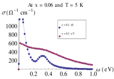
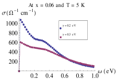
(a)	(b)
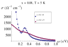
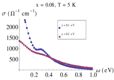
(c)	(d)
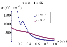
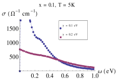
(e)	(f)

Figure 5: (a) Optical conductivity (in $\Omega^{-1}cm^{-1}$) vs frequency (in $eV$) at $x=0.06$ and at temperature $T=5K$. Comparison at different $\gamma$ but with psuedogap. The value of the Drude scattering rate is given in the legend. All the energy scales are measured in $eV$. Figures in the second and 3rd row are for $x=0.08$ and $x=0.1$ respectively. In all figures $t_{0}=0.45eV$.

For the computation we needed a number of parameters of CNCOC system. These are taken from the literatureyrzi ; matt ; car and tabulated below (Table I).

Table 1: Various parameters for CNCOC system.

$CuO$-bond  a-axis	b-axis	c-axis	$t_{0}$
$\simeq 3.87~{}\AA$	$\simeq 3.87~{}\AA$	$\simeq 15~{}\AA$	$\simeq 0.45~{}eV$
$\mu_{p}$ at $x=0.06$	$\mu_{p}$ at $x=0.08$	$\mu_{p}$ at $x=0.1$
$\simeq-0.2~{}eV$	$\simeq-0.23~{}eV$	$\simeq-0.25~{}eV$

The superexchange constant is $J\simeq 0.13~{}eV$ for $Sr_{2}CuO_{2}Cl_{2}$ and for most of the cuprates $t_{0}$ is in $0.3~{}eV\lesssim t_{0}\lesssim 0.5~{}eV$. Here we take $t_{0}=0.45~{}eV$car . At $x=0.05$, $\Delta_{pg}^{0}=180~{}meV$, ARPES do detect this pseudogap ($\Delta^{ARPES}_{pg}\simeq 200~{}meV$) at this doping around the point $(\pi,0)$ in the brillion zone and also co-existing nodal metalarpes .

For numerical computation we considered a 3-D sample of $100\times 100\times 100$ lattice points (thus with sample length, width, and hight: $100a$, $100a$, and $100c$ (where $a$ is the $a$-axis ($a=b$) and $c$ is the $c$-axis lattice constant)). This size of the sample is sufficiently large (as has been numerically verified) and size effects can be neglected. After performing the sum over $k_{z}$ in equation (3) we obtain

$$\sigma(\omega,T)=\frac{4\pi e^{2}\hbar}{N^{2}ca^{2}}\sum_{k_{x}=-\frac{\pi}{a},k_{y}=-\frac{\pi}{a}}^{+\frac{\pi}{a},+\frac{\pi}{a}}v_{o,x}^{2}(k_{x},k_{y})\times$$ (8)

$$\int_{-\infty}^{+\infty}dy\frac{f(y)-f(\omega+y)}{\omega}A(k_{x},k_{y},y)A(k_{x},k_{y},\omega+y).\$$

Here we have redefined the units, now the frequency $y,~{}\omega$ is measured in $eV$ and $\{k_{x},k_{y}\}=-\frac{\pi}{a},-\frac{\pi}{a}+\delta,...,+\frac{\pi}{a}$, with $\delta=\frac{\pi}{Na}$, $N=100$. And the spectral function is

$$A(k_{x},k_{y},\omega)=\frac{\gamma}{(\omega-\epsilon(k_{x},k_{y})-\Sigma_{pg}(k_{x},k_{y},\omega))^{2}+\gamma^{2}}.$$ (9)

Here $\gamma$ and $\omega$ measured in energy units (in $eV$). Band dispersion and self energy is also measured in $eV$ and conductivity has the right units $\Omega^{-1}cm^{-1}$.

Numerical computation is done on Mathematica-$8$ numerically by writing a small program.

In Fig. (5(a)) we plot optical conductivity as a function of frequency at two different $\gamma$’s and at temperature $T=5~{}K$ and hole doping $x=0.06$. Dip seen at around $0.2~{}eV$ is a signature of pseudogap which broadens with increasing $\gamma$ (red solid squares for $\gamma=0.3~{}eV$ and blue filled circles for $\gamma=0.1t_{0}~{}eV$). This pseudogap signature (Dip at around $0.2~{}eV$) disappears at higher temperature. This is shown in Fig. (6(a)) where $T=300~{}K$ and we do not have pseudogap at this temperature. The conductivity obtained at $\gamma=0.3~{}eV$ resembles closely what has been experimentally found (Fig.(8) of Waku etal.waku ). We will see in the next section that although it appears qualitatively in agreement with what has been found experimentally but careful examination shows inconsistencies with YRZ. The other figures are plotted for $x=0.08$ and $x=0.1$ as written in the figure titles.

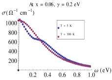
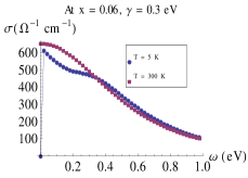
(a)	(b)
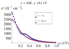
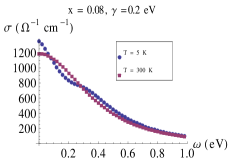
(c)	(d)

Figure 6: (a) With and without pseudogap at $x=0.06$ and $\gamma=0.2~{}eV$. Other plots are at different values of $x$ and $\gamma$ as written in plot titles.

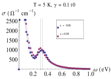
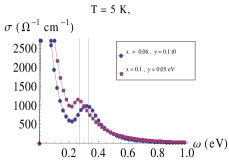
(a)	(b)

Figure 7: With increasing doping $x$, size of the pseudogap decreses $\Delta^{0}_{pg}(x)=0.6t_{0}(1-x/0.2)$. This should result in leftward shifting of the gap signature in the optical conductivity. Figure (a) show this shifting for $x_{1}=0.06$ and $x_{2}=0.08$. Shift in $\Delta^{0}_{pg}(x)$ is $\delta\Delta^{0}_{pg}(x)=3t_{0}(x_{2}-x_{1})\simeq 0.03eV$. This roughly agrees with shift in the graph (the distance between x-axis ticks is $0.05eV$). (b) Shifting for $x=0.06$ and $x=0.1$. Here also $\delta\Delta^{0}_{pg}(x)=3t_{0}(x_{2}-x_{1})\simeq 0.054$. This also roughly agrees with shift in the graph.

In Fig. (7(a)) we plot optical conductivity as a function of frequency at two different doping levels ($x=0.06$, and $x=0.08$) and at temperature $T=5~{}K$ and at $\gamma=0.1t_{0}$. There is a clear shifting of the pseudogap bump to lower frequencies with increasing doping $x$. This is consistent with decreasing $\Delta^{0}_{pg}(x)=0.6t_{0}(1-x/0.2)$ with increasing $x$. In Fig. (7(b)) the same shifting is shown for $x=0.06$ and $x=0.1$. Shifting seen in the graph agrees with $\delta\Delta^{0}_{pg}(x)=3t_{0}(x_{2}-x_{1})\simeq 0.054$ as explained in figure caption. This shifting of pseudogap signature in conductivity results similar shifting of the signature of pseudogap in the generalized Drude model scattering rate. But, in contrast, this kind of shifting is not seen in the experiment of Waku etalwaku . This is the subject of the next section.

IV Extended Drude model analysis and inconsistencies with YRZ model

In this section we will show that optical conductivity as computed using YRZ is inconsistent with what has been experimentally observed inwaku . We will deduce the above statement by the method of reductio ad absurdum of logic, i.e., proof by contradiction. So let us assume that YRZ is the correct model for the computation of optical conductivity in the low frequency regime which we are considering, i.e., the underlying transport properties of quasi-particles are captured by YRZ. Now, as done in the experimental paper by Waku etal.waku we analyze the optical conductivity from YRZ ansatz with the extended Drude model and extract the frequency dependent scattering rate. If the scattering rate so deduced agrees with scattering rate deduced with similar analysis of the experimental data, then, YRZ ansatz is consistent with what has been experimentally observed, otherwise,it is not.

Now, as mentioned before (below equation (7)), theywaku deduce frequency dependence of the scattering rate $\Gamma(\omega)$ of extended Drude model by using their experimental data. They found that at low frequencies $\hbar\omega\lesssim 0.4~{}eV$ scattering rate is almost proportional to $\omega$ ($\Gamma(\omega)=\Gamma_{0}+C\omega$) and $C$ turns out to be almost temperature independent. And $\Gamma_{0}$ increases with increasing temperature (refer to figure (10) in their paperwaku ). They see that above $\hbar\omega\gtrsim 0.4~{}eV$ the scattering rate saturates to a constant value.

In our case, the scattering rate can be computed frombasov :

$$\Gamma_{gd}(\omega) \equiv \frac{1}{\tau(\omega)}=\frac{ne^{2}}{m^{\ast}}Re\left(\frac{1}{\tilde{\sigma}(\omega)}\right)$$ (10)

$$= \frac{ne^{2}}{m^{\ast}}\frac{\sigma(\omega)}{(\sigma(\omega))^{2}+(\sigma_{im}(\omega))^{2}}.$$

For this we need to compute imaginary part of conductivity $\sigma_{im}(\omega)$ (real part is $\sigma(\omega)$). As we are dealing with the casual perturbation and response relationship, the real and imaginary parts are related by Kramers-Kronig relations. By doing a numerical Kramers-Kronig inversion we obtain $\sigma_{im}(\omega)$ (as plotted in Fig. (8(a))) and then we calculate $\Gamma_{gd}$. In Fig. (8(b)) we plot $\Gamma(\omega)=\frac{\sigma(\omega)}{(\sigma(\omega))^{2}+(\sigma_{im}(\omega))^{2}}$; ($\Gamma_{gd}(\omega)=\frac{ne^{2}}{m^{\ast}}\Gamma(\omega)$) at $\gamma=0.2~{}eV$.

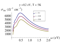
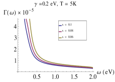
(a)	(b)

Figure 8: (a) Imaginary part of conductivity $\sigma_{im}(\omega)$ calculated from the real part by Kramers-Kronig transformation. The scattering rate $\gamma$ and temperature $T$ is fixed at $0.2eV$ and $5K$ in these two graphs. The calculation is done for hole dopings $x=0.06$, $x=0.08$, and $x=0.1$. We see that higher the doping higher is the conductivity and the peak in conductivity shifts to lower frequencies with increasing doping as is investigated in figure (7). The scattering rate $\Gamma(\omega)$ obtained from extended Drude model monotonically decrease with increasing frequency. This is in sharp contrast with the experimental observations of Waku et alwaku where $\Gamma(\omega)$ first increases linearly with frequency and then saturates at around $\omega_{c}\sim 0.4eV$.

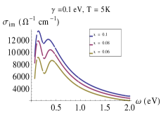
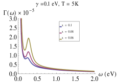
(a)	(b)

Figure 9: The similar analysis as in figure 8 with $\gamma=0.1$.

We see clearly from Fig. (8(b)) that the scattering rate $\Gamma(\omega)$ obtained from extended Drude model monotonically decrease with increasing frequency. This is in sharp contrast with the experimental observations of Waku et alwaku where $\Gamma(\omega)$ first increases linearly with frequency and then saturates at around $\omega_{c}\sim 0.4eV$. Also with reduced doping $\Gamma(\omega)$ shifts to lower $\hbar\omega$ in numerical study. Comparison of Fig. 4(b) (or figure (10) inwaku ) with Fig. 8(b) clearly points out the inconsistencies. The smeared out features of the pseudogap at higher $\gamma$ ($\gamma=0.2~{}eV$ in Fig. (8)) can be seen at lower $\gamma$ ($\gamma=0.1~{}eV$ in Fig. (9)). But the pseudogap peak in $\Gamma(\omega)$ shifts to higher $\hbar\omega$ with reduced doping (similar to the shift of $\sim 0.05~{}eV$ between the peaks at $x=0.06$ and $x=0.1$ in Fig. 7(b)). Also the behaviour of two scattering rates ( Fig. 4(b) and Fig. 9(b)) is qualitatively different.

V Conclusion

We theoretically investigated charge dynamics in weakly coupled $CuO_{2}$ planes of the cuprate $Ca_{2-x}Na_{x}CuO_{2}Cl_{2}$ (CNCOC) using YRZ ansatz for the single particle Green’s function in the pseudogap state. To an unaided eye, the results of our numerical calculation appears to be in qualitative agreement with what has been found experimentally inwaku . But a careful examination with extended Drude formalism shows that YRZ ansatz for the calculation of optical conductivity is not sufficient to understand the optical conductivity in $CuO_{2}$ planes of the compound CNCOC. It seems that more physics is needed to fully understand the optical response especially the response from bound charges.

References

- (1) K. Waku, T. Katsufuji, Y. Kohsaka, T. Sasagawa, H. Takagi, H. Kishida, H. Okamoto, M. Azuma, and M. Takano, Phys. Rev. B 70, 134501 (2004).
- (2) P. W. Anderson, P. A. Lee, M. Randeria, T. M. Rice, N. Trivedi, and F. C. Zhang, J. Phys. Condens. Matter 16, R755 (2004); P. A. Lee, N. Nagaosa, and X. G. Wen, Rev. Mod. Phys. 78, 17 (2006); M. Ogata, and H. Fukuyama, Rep. Prog. Phys. 71, 036501 (2008); P. W. Anderson, Int. J. Mod. Phys. B 25, 1 (2011).
- (3) Elbio Dagotto, Rev. Mod. Phys. 66, 763 (1994).
- (4) M. R. Norman, D. Pines, and C. Kallin, Adv. Phys. 54, 715 (2005); A. J. Leggett, Nat. Phys. 2, 134 (2006); J. P. Carbotte, T. Timusk, J. Hwang, Rep. Prog. Phys. 74, 066501/1-43 (2011); O. Gunnarsson, O. Rosch, J. Phys.: Condens. Matter 20, 043201 (2008).
- (5) T. M. Rice, K. Y. Yang, and F. C. Zhang, Rep. Prog. Phys. 75, 016502 (2012).
- (6) K. Y. Yang, T. M. Rice, and F. C. Zhang, Phys. Rev. B 73, 174501 (2006).
- (7) F. C. Zhang, C. Gros, T. M. Rice, and H. Shiba, Supercond. Sci. Technol. 1 36-46 (1988).
- (8) E. Dagotto and T. M. Rice, Science, 271, 618 (1996); R. M. Konik and A. W. W. Ludwig, Phys. Rev. B. 64, 155112 (2001); R. M. Konik, T. M. Rice, and A. M. Tsvelik, Phys. Rev. Lett. 96, 086407 (2006).
- (9) K. M. Shen, F. Ronning, D. H. Lu, F. Baumberger, N. J. C. Ingle, W. S. Lee, W. Meevasana, Y. Kohsaka, M. Azuma, M. Takano, H. Takagi, Z.-X. Shen, Science, 307, 901 (2005).
- (10) H. B. Yang, J. D. Rameau, P. D. Johnson, T. Valla, A. Tsvelik, and G. D. Gu, Nature, 456 77 (2008); H. B. Yang, J. D. Rameau, Z. H. Pan, G. D. Gu, P. D. Johnson, R. H. Claus, D. G. Hinks, and T. E. Kidd, Phys. Rev. Lett. 107 047003 (2011).
- (11) M. Hashimoto, T. Yoshida, K. Tanaka, A. Fujimori, M. Okusawa, S. Wakimoto, K. Yamada, T. Kakeshita, H. Eisaki, and S. Uchida, Phys. Rev. B 79 140502 (2009).
- (12) Y. Kohsaka, C. Taylor, P. Wahl, A. Schmidt, L. Jhinhwan, K. Fujita, J. W. Alldredge, K. McElroy, L. Jinho, H. Eisaki, S. Uchida, D. H. Lee, and J. C. Davis, Nature 454 1072 (2008).
- (13) T. P. Devereaux and R. Hackl, Rev. Mod. Phys. 79, 175 (2007).
- (14) B. Valenzuela and Elena Bascones, Phys. Rev. Lett. 98, 227002 (2007).
- (15) M. L. Tacon, A. Sacuto, A. Georges, G. Kotliar, Y. Gallais, D. Colson, and A. Forget, Nat. Phys. 2, 537 (2006).
- (16) M. R. Norman, M. Randeria, H. Ding, and J. C. Campuzano, Phys. Rev. B 57 11093(R) (1998); S. Banerjee, T. V. Ramakrishnan, and C. Dasgupta, Phys. Rev. B 84, 144525 (2011); Also see discussion on page 35 of yrzrev .
- (17) M. Tinkham, Rev. Mod. Phys. 46, 587 (1974).
- (18) D. C. Mattis and J. Bardeen, Phys. Rev. 111, 412 (1958).
- (19) E. Illes, E. J. Nicol, and J. P. Carbotte, Phys. Rev. B 79, 100505(R) (2009); A. Pound, J. P. Carbotte, E. J. Nicol, Eur. Phys. J. B 81, 69 (2011).
- (20) F. C. Zhang and T. M. Rice, Phys. Rev. B 37, 3759 (1988).
- (21) V. J. Emery, G. Reiter, Phys. Rev. B 38, 11938 (1988); F. C. Zhang and T. M. Rice, Phys. Rev. B 41, 7243 (1990); V. J. Emery, G. Reiter, Phys. Rev. B 41, 7247 (1990); Seedagotto and references therein.
- (22) R. Konik and A. W. W. Ludwig, Phys. Rev. B 64, 155112 (2001); R. Konik, T. M. Rice, and A. M. Tsvelik, Phys. Rev. Lett. 96, 086407 (2006).
- (23) Gerald D. Mahan, Many Particle Physics (Physics of Solids and Liquids), Springer; 3rd edition (2000).
- (24) L. F. Mattheiss, Phys. Rev. B. 42, 354 (1990).
- (25) D. N. Basov and T. Timusk, Rev. Mod. Phys. 77, 721 (2005); J. W. Allen and J. C. Mikkelsen, Phys. Rev. B. 15, 2952 (1976); W. Gotze, Philos. Mag. B. 43, 219 (1981).