The n-order rogue waves of Fokas-Lenells equation

Abstract.

Considering certain terms of the next asymptotic order beyond the nonlinear Schrödinger equation (NLS) equation, the Fokas-Lenells (FL) equation governed by the FL system arise as a model for nonlinear pulse propagation in optical fibers. The expressions of the $q^{[n]}$ and $r^{[n]}$ in the FL system are generated by n-fold Darboux transformation (DT), each element of the matrix is a 2 2 matrix, expressed by a ratio of $(2n+1)\times(2n+1)$ determinant and $2n\times 2n$ determinant of eigenfunctions. Further, a Taylor series expansion about the n-order breather solutions $q^{[n]}$ generated using DT by assuming periodic seed solutions under reduction can generate the n-order rogue waves of the FL equation explicitly with $2n+3$ free parameters.

Key words: the nonlinear Schrödinger equation, Fokas-Lenells equation,
                           Darboux transformation, breather solution, rogue wave.

PACS(2010) numbers: 02.30.Ik, 42.81.Dp, 52.35.Bj, 52.35.Sb, 94.05.Fg

MSC(2010) numbers: 35C08, 37K10, 37K40

1. introduction

The Fokas-Lenells equation (FL)[1, 2, 3, 5, 4]

$$iq_{xt}-iq_{xx}+2q_{x}-q_{x}qq^{\ast}+iq=0,$$ (1)

is one of the important models from both mathematical and physical considerations. In eq.(1), $q$ represents the complex field envelope and asterisk denotes its complex conjugation, the subscript $x$ (or $t$) denotes partial derivative with respect to $x$ (or $t$). The FL equation [1, 3] is related to the nonlinear Schrödinger (NLS) equation in the same way as the Camassa-Holm equation associated with the KdV equation. The authors of [3] , after deriving associated Lax pair and using initial value problem, they were able to solve the equation. The soliton solutions of the FL equation have been constructed via the Riemann-Hilbert method in [2] and through dressing method in [5]. The breather solutions of the FL equation have also been constructed via a dressing-Backlund transformation related to the Riemann-Hilbert problem formulation of the inverse scattering theory [6]; also in the same paper three instability regions were analyzed, associated with a single unstable wave number. The FL equation actually describes the first negative flow of the integrable hierarchy associated with the derivative nonlinear Schrödinger (DNLS) equation [4] (it also belongs to the deformed DNLS hierarchy proposed by A.Kundu [7, 8]). The lattice representation and the dark solitons of the FL equation have been presented in [9], where a relationship is also established between the FL equation and other integrable models including the NLS equation, the Merola-Ragnisco-Tu equations and the Ablowitz-Ladik equation. Recently, it has been shown that the periodic initial value problem for the FL equation is well-posed in a Sobolev space with exponent greater than 3/2[10]. In optics, considering suitable higher order linear and nonlinear optical effects, the FL equation has been derived as a model to describe the femtosecond pulse propagation through single mode optical silica fiber and several interesting solutions have been constructed [4].

Rogue waves have recently been the subject of intensive investigations in oceanography[11, 12, 13], where they occur due to either modulation instability [14, 15, 16], or other processes[17, 18, 19]. The first order rogue wave usually takes the form of a single peak hump with two caves in a plane with a nonzero boundary. One of the possible generating mechanisms for rogue waves is through the creation of breathers which can be formed as a consequence of modulation instability. Then, larger rogue waves can emerge when two or more breathers collide with each other[20, 21, 22]. Rogue waves have also been observed in space plasmas[23, 24, 25, 26, 27], as well as in optics when propagating high power optical radiation through photonic crystal fibers [28, 29, 30]. Though the rogue waves have been reported in different branches of physics where the system dynamics is governed by single equation, to the best our knowledge, they have been observed and reported very little in the coupled systems. For example, Rogue waves of the coupled Schrödinger equations are construct in the literature[31, 32, 33]. In experiment, the rogue waves in a multistable system [34] is revealed by experiments with an erbium-doped fiber laser driven by harmonic pump modulation. Considering higher order effects in the propagation of femtosecond pulses, rogue waves have been reported in the Hirota equation[35, 36] and in resonant erbium-doped fibre system governed by a coupled system of the nonlinear Schrödinger equation and the Maxwell-Bloch (NLS-MB) equations[37]. Very recently, the new types of matter rogue waves [38] have been reported in $F=1$ spinor Bose-Einstein condensate governed by a three-component NLS equations. Some interesting results on the multi-rogue wave solutions of the NLS equation have also been done in [39, 40, 41, 42, 43, 44, 45], which shows that there exist many patterns of the rogue waves and their formulae have extreme complexity.

Considering the physical significance of the FL equation, inspired by the importance of the recent interesting developments in the rogue waves of the NLS type equations, so we have reported the first order rogue wave[46] of the FL equation in by Darboux transformation (DT)[47, 48, 49]. Our construction reveals that there exists some deviations in their solutions and DT between the FL system and other integrable models such as Ablowitz-Kaup-Newell-Segur (AKNS) system[50, 51] and Kaup-Newell (KN) system[52, 53, 54]. The purpose of this paper is to provide a detailed derivation of the determinant representation of the N-fold DT of the FL equation as we have done for the case of NLS equation [49], which will be used to construct higher order rogue wave. Several different patterns of the higher order rogue waves will be plotted according to the determinant representation.

The organization of this paper is as follows. In section 2, it provides a relatively simple approach to DT for the FL system, which is followed by the determinant representation of the n-fold DT and formulae of $q^{[n]}$ and $r^{[n]}$ expressed by eigenfunctions of spectral problem are given. The reduction of DT of the FL system to the FL equation is also discussed by choosing paired eigenvalues and eigenfunctions. In section 3, a Taylor series expansion about the n-order breather solutions generated by DT from a periodic seed solution with a constant amplitude can construct the n-order rogue waves of the FL equation in the determinant forms with $2n+3$ free parameters. Finally, we conclude the results in section 4.

2. Darboux transformation

Let us start from the non-trivial flow of the FL (Fokas-Lenells) system[3],

$$iq_{xt}-iq_{xx}+2q_{x}-q_{x}qr+iq=0,$$ (2)

$$ir_{xt}-ir_{xx}-2r_{x}+r_{x}rq+ir=0,$$ (3)

which are exactly reduced to the FL eq.(1) for $r=q^{\ast}$ while the choice $r=-q^{\ast}$ would lead to eq.(1) with the sign of the nonlinear term changed. The Lax pairs corresponding to coupled FL eq.(2) and (3) can be given by the FL spectral problem[3]

$$\partial_{x}\psi=(J\lambda^{2}+Q\lambda)\psi=U\psi,$$ (4)

$$\partial_{t}\psi=(J\lambda^{2}+Q\lambda+V_{0}+V_{-1}\lambda^{-1}+\dfrac{1}{4}J\lambda^{-2})\psi=V\psi,$$ (5)

with

$$\psi=\left(\begin{array}[]{c}\phi\\ \varphi\\ \end{array}\right),\\ \quad J=\left(\begin{array}[]{cc}-i&0\\ 0&i\\ \end{array}\right),\\ \quad Q=\left(\begin{array}[]{cc}0&q_{x}\\ r_{x}&0\\ \end{array}\right),\\$$

$$V_{0}=\left(\begin{array}[]{cc}i-\frac{1}{2}iqr&0\\ 0&-i+\frac{1}{2}iqr\\ \end{array}\right),\quad V_{-1}=\left(\begin{array}[]{cc}0&\frac{1}{2}iq\\ -\frac{1}{2}ir&0\\ \end{array}\right).\\$$

Here $\lambda$ is an arbitrary complex number, called the eigenvalue(or spectral parameter), and $\psi$ is called the eigenfunction associated with $\lambda$ of the FL system. Equations (2) and (3) are equivalent to the integrability condition $U_{t}-V_{x}+[U,V]=0$ of (4) and (5).

The main task of this section is to present a detailed derivation of the DT of the FL equation and the determinant representation of the n-fold transformation. Based on the DT for the NLS[47, 48, 49] and the DNLS[53, 54, 26, 27], the main steps are : 1) finding $2\times 2$ matrix $T$ so that the FL spectral problem eq.(4) and eq.(5) is covariant, then get new solution $(q^{[1]},r^{[1]})$ expressed by elements of $T$ and seed solution $(q,r)$; 2) finding the expressions of elements of $T$ in terms of eigenfunctions of FL spectral problem corresponding to the seed solution $(q,r)$; 3) to get the determinant representation of n-fold DT $T_{n}$ and new solutions $(q^{[n]},r^{[n]})$ by $n$-times iteration of the DT; 4) to consider the reduction condition: $q^{[n]}=(r^{[n]})^{*}$ by choosing special eigenvalue $\lambda_{k}$ and its eigenfunction $\psi_{k}$, and then get $q^{[n]}$ of the FL equation expressed by its seed solution $q$ and its associated eigenfunctions $\{\psi_{k},k=1,2,\cdots,n\}$. However, we shall use the kernel of n-fold DT($T_{n}$) to fix it in the third step instead of iteration.

It is straightforward to see that the spectral problem (4) and (5) are transformed to

$${\psi^{[1]}}_{x}=U^{[1]}~{}\psi^{[1]},\ \ U^{[1]}=(T_{x}+T~{}U)T^{-1}.$$ (6)

$${\psi^{[1]}}_{t}=V^{[1]}~{}\psi^{[1]},\ \ V^{[1]}=(T_{t}+T~{}V)T^{-1}.$$ (7)

under a gauge transformation

$$\psi^{[1]}=T~{}\psi.$$ (8)

By cross differentiating (6) and (7), we obtain

$${U^{[1]}}_{t}-{V^{[1]}}_{x}+[{U^{[1]}},{V^{[1]}}]=T(U_{t}-V_{x}+[U,V])T^{-1}.$$ (9)

This implies that, in order to make eqs.(2) and (3) invariant under the transformation (8), it is crucial to search a matrix $T$ so that $U^{[1]}$, $V^{[1]}$ have the same forms as $U$, $V$. At the same time the old potential(or seed solution)($q$, $r$) in spectral matrixes $U$, $V$ are mapped into new potentials(or new solution)($q^{[1]}$, $r^{[1]}$) in transformed spectral matrixes $U^{[1]}$, $V^{[1]}$.

2.1 One-fold Darboux transformation of the FL system

Considering the universality of DT, suppose that the trial Darboux matrix $T$ in eq.(8) is of the form

$$T=T(\lambda)=\left(\begin{array}[]{cc}a_{1}&b_{1}\\ c_{1}&d_{1}\\ \end{array}\right)\lambda+\left(\begin{array}[]{cc}a_{0}&b_{0}\\ c_{0}&d_{0}\\ \end{array}\right)+\left(\begin{array}[]{cc}a_{-1}&b_{-1}\\ c_{-1}&d_{-1}\\ \end{array}\right)\lambda^{-1},$$ (10)

where $a_{-1},b_{-1},c_{-1},d_{-1},a_{0},b_{0},c_{0},d_{0},a_{1},b_{1},c_{1},d_{1}$ are functions of $x$ and $t$. From

$$T_{x}+T~{}U=U^{[1]}~{}T,$$ (11)

comparing the coefficients of $\lambda^{j},j=3,2,1,0,-1$, it yields

$$\lambda^{3}:b_{1}=0,\ c_{1}=0,$$

$$\lambda^{2}:q_{x}~{}a_{1}+2~{}i~{}b_{0}-{q^{[1]}}_{x}d_{1}=0,\ -{r^{[1]}}_{x}~{}a_{1}+r_{x}~{}d_{1}-2~{}i~{}c_{0}=0,$$

$$\lambda^{1}:{a_{1}}_{x}+r_{x}~{}b_{0}-{q^{[1]}}_{x}c_{0}=0,\ {d_{1}}_{x}+q_{x}c_{0}-{r^{[1]}}_{x}b_{0}=0,$$

$$\mbox{\hskip 19.91684pt}q_{x}a_{0}-{q^{[1]}}_{x}d_{0}+2ib_{-1}=0,-{r^{[1]}}_{x}a_{0}+r_{x}d_{0}-2ic_{-1}=0,$$

$$\lambda^{0}:-q^{[1]}c_{-1}+r_{x}b_{-1}+{a_{0}}_{x}=0,-q^{[1]}d_{-1}+q_{x}a_{-1}+{b_{0}}_{x}=0,$$

$$\mbox{\hskip 19.91684pt}-r^{[1]}a_{-1}+r_{x}d_{-1}+{c_{0}}_{x}=0,-r^{[1]}b_{-1}+q_{x}c_{-1}+{d_{0}}_{x}=0,$$

$$\lambda^{-1}:{a_{-1}}_{x}={b_{-1}}_{x}={c_{-1}}_{x}={d_{-1}}_{x}=0.$$ (12)

The terms in the previous equation $a_{-1},b_{-1},c_{-1},d_{-1}$ are all functions of $t$ only. Similarly, from

$$T_{t}+T~{}V=V^{[1]}~{}T,$$ (13)

comparing the coefficients of $\lambda^{j},j=2,1,0,-1,-2,-3$ under the condition $b_{1}=c_{1}=0$, it implies

$$\lambda^{-3}:b_{-1}=c_{-1}=0,$$

$$\lambda^{-2}:-q^{[1]}d_{-1}+qa_{-1}+b_{0}=0,-r^{[1]}a_{-1}+rd_{-1}+c_{0}=0,$$

$$\lambda^{-1}:{a_{-1}}_{t}-\dfrac{1}{2}iq^{[1]}c_{0}+\frac{1}{2}iq^{[1]}r^{[1]}a_{-1}-\frac{1}{2}iqra_{-1}-\frac{1}{2}irb_{0}=0,-q^{[1]}d_{0}+qa_{0}=0,$$

$$\mbox{\hskip 22.76228pt}{d_{-1}}_{t}+\dfrac{1}{2}ir^{[1]}b_{0}-\frac{1}{2}iq^{[1]}r^{[1]}d_{-1}+\frac{1}{2}iqrd_{-1}+\frac{1}{2}iqc_{0}=0,-r^{[1]}a_{0}+rd_{0}=0,$$

$$\lambda^{0}:{a_{0}}_{t}-\dfrac{1}{2}iqra_{0}+\frac{1}{2}iq^{[1]}r^{[1]}a_{0}=0,{d_{0}}_{t}+\dfrac{1}{2}iqrd_{0}-\frac{1}{2}iq^{[1]}r^{[1]}d_{0}=0,$$

$$\mbox{\hskip 22.76228pt}q_{x}a_{-1}+\frac{1}{2}iqa_{1}-2ib_{0}-\frac{1}{2}iq^{[1]}d_{1}+{b_{0}}_{t}-{q^{[1]}}_{x}d_{-1}+\frac{1}{2}iq^{[1]}r^{[1]}b_{0}+\frac{1}{2}iqrb_{0}=0,$$

$$\mbox{\hskip 22.76228pt}r_{x}d_{-1}-\frac{1}{2}ird_{1}+2ic_{0}+\frac{1}{2}ir^{[1]}a_{1}+{c_{0}}_{t}-{r^{[1]}}_{x}a_{-1}-\frac{1}{2}iq^{[1]}r^{[1]}c_{0}-\frac{1}{2}iqrc_{0}=0,$$

$$\lambda^{1}:-{q^{[1]}}_{x}d_{0}+q_{x}a_{0}=0,-{r^{[1]}}_{x}a_{0}+r_{x}d_{0}=0,$$

$$\mbox{\hskip 22.76228pt}\dfrac{1}{2}iq^{[1]}r^{[1]}a_{1}-\frac{1}{2}iqra_{1}+{a_{1}}_{t}+r_{x}b_{0}-{q^{[1]}}_{x}c_{0}=0,$$

$$\mbox{\hskip 17.07182pt}-\dfrac{1}{2}iq^{[1]}r^{[1]}d_{1}+\frac{1}{2}iqrd_{1}+{d_{1}}_{t}+q_{x}c_{0}-{r^{[1]}}_{x}b_{0}=0,$$

$$\lambda^{2}:q_{x}a_{1}-q^{[1]}_{x}d_{1}+2ib_{0}=0,r_{x}d_{1}-q^{[1]}_{x}a_{1}-2ic_{0}=0.$$ (14)

In order to get the non-trivial solutions, we shall construct a basic (or one-fold) DT matrix $T$ under an assumption that $a_{0}=0$ and $d_{0}=0$. If we set $a_{0}\not=0$, then we can get that $d_{0}$ is not zero by $-q^{[1]}d_{0}+qa_{0}=0$ and $-q^{[1]}d_{0}+qa_{0}=0$ from eq.(2), and furthermore find that some coefficients of $a_{0}$ and $d_{0}$ are constants by taking $q^{[1]}=q\dfrac{a_{0}}{d_{0}}$ and $r^{[1]}=r\dfrac{d_{0}}{a_{0}}$ into eq.(2) and eq.(2), which gives a trivial solution. What is more, we can learn those equation $q_{x}~{}a_{1}+2~{}i~{}b_{0}-{q^{[1]}}_{x}d_{1}=0$, $-{r^{[1]}}_{x}~{}a_{1}+r_{x}~{}d_{1}-2~{}i~{}c_{0}=0$,$-q^{[1]}d_{-1}+qa_{-1}+b_{0}=0$ and $-r^{[1]}a_{-1}+rd_{-1}+c_{0}=0$ from eq.(2) and eq.(2). Under the condition $a_{1}d_{1}a_{-1}d_{-1}\neq 0$,we can get that $a_{-1}$ , $d_{-1}$, $a_{1}$ and $d_{1}$ are constants from eq.(2) and eq.(2). This means that our assumption does not suppresses the generality of the DT of the FL system. Based on eq.(2) and (2) and above analysis, let Darboux matrix $T$ be the form of

$$T_{1}=T_{1}(\lambda;\lambda_{1};\lambda_{2})=\left(\begin{array}[]{cc}a_{1}&0\\ 0&d_{1}\\ \end{array}\right)\lambda+\left(\begin{array}[]{cc}0&b_{0}\\ c_{0}&0\\ \end{array}\right)+\left(\begin{array}[]{cc}a_{-1}&0\\ 0&d_{-1}\\ \end{array}\right)\lambda^{-1}.$$ (15)

Here $a_{1},d_{1},b_{0},c_{0}$ are undetermined function of ($x$, $t$), which will be expressed by the eigenfunction associated with $\lambda_{1}$ and $\lambda_{2}$ in the FL spectral problem, and $a_{-1},d_{-1}$ are constants. First of all, we introduce $n$ eigenfunctions $\psi_{j}$ as

$$\psi_{j}=\left(\begin{array}[]{c}\phi_{j}\\ \varphi_{j}\\ \end{array}\right),\ \ j=1,2,....n,\phi_{j}=\phi_{j}(x,t,\lambda_{j}),\ \varphi_{j}=\varphi_{j}(x,t,\lambda_{j}).$$ (18)

Theorem 1.The elements of one-fold DT are parameterized by the eigenfunction $\psi_{i}$ ($i=1,2$) associated with $\lambda_{i}$, as follows

$$T_{1}(\lambda;\lambda_{1};\lambda_{2})=\left(\begin{array}[]{cc}a_{1}\lambda+a_{-1}\lambda^{-1}&b_{0}\\ c_{0}&d_{1}\lambda+d_{-1}\lambda^{-1}\end{array}\right),$$ (21)

and then the new solutions $q^{[1]}$ and $r^{[1]}$ are given by

$$q^{[1]}=q\dfrac{a_{-1}}{d_{-1}}+\dfrac{b_{0}}{d_{-1}},r^{[1]}=r\dfrac{d_{-1}}{a_{-1}}+\dfrac{c_{0}}{a_{-1}},$$ (22)

with $a_{-1}=1,d_{-1}=1$ and

$$a_{1}=\dfrac{\begin{vmatrix}-{\lambda_{1}}^{-1}\phi_{1}&\varphi_{1}\\ -{\lambda_{2}}^{-1}\phi_{2}&\varphi_{2}\\ \end{vmatrix}}{\begin{vmatrix}\lambda_{1}\phi_{1}&\varphi_{1}\\ \lambda_{2}\phi_{2}&\varphi_{2}\\ \end{vmatrix}},\quad d_{1}=\dfrac{\begin{vmatrix}-{\lambda_{1}}^{-1}\varphi_{1}&\phi_{1}\\ -{\lambda_{2}}^{-1}\varphi_{2}&\phi_{2}\\ \end{vmatrix}}{\begin{vmatrix}\lambda_{1}\varphi_{1}&\phi_{1}\\ \lambda_{2}\varphi_{2}&\phi_{2}\\ \end{vmatrix}},\quad b_{0}=\dfrac{\begin{vmatrix}\lambda_{1}\phi_{1}&-{\lambda_{1}}^{-1}\phi_{1}\\ \lambda_{2}\phi_{2}&-{\lambda_{2}}^{-1}\phi_{2}\\ \end{vmatrix}}{\begin{vmatrix}\lambda_{1}\phi_{1}&\varphi_{1}\\ \lambda_{2}\phi_{2}&\varphi_{2}\\ \end{vmatrix}},\quad c_{0}=\dfrac{\begin{vmatrix}\lambda_{1}\varphi_{1}&-{\lambda_{1}}^{-1}\varphi_{1}\\ \lambda_{2}\varphi_{2}&-{\lambda_{2}}^{-1}\varphi_{2}\\ \end{vmatrix}}{\begin{vmatrix}\lambda_{1}\varphi_{1}&\phi_{1}\\ \lambda_{2}\varphi_{2}&\phi_{2}\\ \end{vmatrix}}$$

and the new eigenfunction $\psi_{j}^{[1]}$ corresponding to $\lambda_{j}$ is

$$\psi^{[1]}_{j}=\left(\begin{array}[]{c}\dfrac{\begin{vmatrix}\lambda_{i}\phi_{i}&-{\lambda_{i}}^{-1}\phi_{i}&\varphi_{i}\\ \lambda_{1}\phi_{1}&-{\lambda_{1}}^{-1}\phi_{1}&\varphi_{1}\\ \lambda_{2}\phi_{2}&-{\lambda_{2}}^{-1}\phi_{2}&\varphi_{2}\\ \end{vmatrix}}{\begin{vmatrix}\lambda_{1}\phi_{1}&\varphi_{1}\\ \lambda_{2}\phi_{2}&\varphi_{2}\\ \end{vmatrix}}\\ \\ \dfrac{\begin{vmatrix}\lambda_{i}\varphi_{i}&-{\lambda_{i}}^{-1}\varphi_{i}&\phi_{i}\\ \lambda_{1}\varphi_{1}&-{\lambda_{1}}^{-1}\varphi_{1}&\phi_{1}\\ \lambda_{2}\varphi_{2}&-{\lambda_{2}}^{-1}\varphi_{2}&\phi_{2}\\ \end{vmatrix}}{\begin{vmatrix}\lambda_{1}\varphi_{1}&\phi_{1}\\ \lambda_{2}\varphi_{2}&\phi_{2}\\ \end{vmatrix}}\end{array}\right).$$

Proof: Note that $a_{-1}$ and $d_{-1}$ are constants, which are derived from the eq.(2) and eq.(2), respectively. From eq.(2) and transformation eq.(15), new solutions are given by

$$q^{[1]}=q\dfrac{a_{-1}}{d_{-1}}+\dfrac{b_{0}}{d_{-1}},r^{[1]}=r\dfrac{d_{-1}}{a_{-1}}+\dfrac{c_{0}}{a_{-1}}$$ (23)

By using a general fact of the DT, (i.e.), $T_{1}(\lambda;\lambda_{1};\lambda_{2})|_{\lambda=\lambda_{i}}\psi_{i}=0,i=1,2$, new solutions are given as eq. (22). Further, by using the explicit matrix representation eq.(21) of $T_{1}$, then $\psi^{[1]}_{j}$ is given by

$$\psi^{[1]}_{j}=T_{1}(\lambda;\lambda_{1};\lambda_{2})|_{\lambda=\lambda_{j}}\psi_{j}=\left.\left(\begin{array}[]{cc}\dfrac{\begin{vmatrix}-{\lambda_{1}}^{-1}\phi_{1}&\varphi_{1}\\ -{\lambda_{2}}^{-1}\phi_{2}&\varphi_{2}\\ \end{vmatrix}}{\begin{vmatrix}\lambda_{1}\phi_{1}&\varphi_{1}\\ \lambda_{2}\phi_{2}&\varphi_{2}\\ \end{vmatrix}}\lambda+\lambda^{-1}&\dfrac{\begin{vmatrix}\lambda_{1}\phi_{1}&-{\lambda_{1}}^{-1}\phi_{1}\\ \lambda_{2}\phi_{2}&-{\lambda_{2}}^{-1}\phi_{2}\\ \end{vmatrix}}{\begin{vmatrix}\lambda_{1}\phi_{1}&\varphi_{1}\\ \lambda_{2}\phi_{2}&\varphi_{2}\\ \end{vmatrix}}\\ \dfrac{\begin{vmatrix}\lambda_{1}\varphi_{1}&-{\lambda_{1}}^{-1}\varphi_{1}\\ \lambda_{2}\varphi_{2}&-{\lambda_{2}}^{-1}\varphi_{2}\\ \end{vmatrix}}{\begin{vmatrix}\lambda_{1}\varphi_{1}&\phi_{1}\\ \lambda_{2}\varphi_{2}&\phi_{2}\\ \end{vmatrix}}&\dfrac{\begin{vmatrix}-{\lambda_{1}}^{-1}\varphi_{1}&\phi_{1}\\ -{\lambda_{2}}^{-1}\varphi_{2}&\phi_{2}\\ \end{vmatrix}}{\begin{vmatrix}\lambda_{1}\varphi_{1}&\phi_{1}\\ \lambda_{2}\varphi_{2}&\phi_{2}\\ \end{vmatrix}}\lambda+\lambda^{-1}\end{array}\right)\right|_{\lambda=\lambda_{j}}\left(\begin{array}[]{c}\phi_{j}\\ \varphi_{j}\end{array}\right)$$ (26)

$$\mbox{\hskip 128.0374pt}=\left(\begin{array}[]{c}\dfrac{\begin{vmatrix}\lambda_{i}\phi_{i}&-{\lambda_{i}}^{-1}\phi_{i}&\varphi_{i}\\ \lambda_{1}\phi_{1}&-{\lambda_{1}}^{-1}\phi_{1}&\varphi_{1}\\ \lambda_{2}\phi_{2}&-{\lambda_{2}}^{-1}\phi_{2}&\varphi_{2}\\ \end{vmatrix}}{\begin{vmatrix}\lambda_{1}\phi_{1}&\varphi_{1}\\ \lambda_{2}\phi_{2}&\varphi_{2}\\ \end{vmatrix}}\\ \\ \dfrac{\begin{vmatrix}\lambda_{i}\varphi_{i}&-{\lambda_{i}}^{-1}\varphi_{i}&\phi_{i}\\ \lambda_{1}\varphi_{1}&-{\lambda_{1}}^{-1}\varphi_{1}&\phi_{1}\\ \lambda_{2}\varphi_{2}&-{\lambda_{2}}^{-1}\varphi_{2}&\phi_{2}\\ \end{vmatrix}}{\begin{vmatrix}\lambda_{1}\varphi_{1}&\phi_{1}\\ \lambda_{2}\varphi_{2}&\phi_{2}\\ \end{vmatrix}}\end{array}\right).$$

After, a tedious calculation shows that $T_{1}$ in eq.(21) and new solutions indeed satisfy eq.(11) and eq.(13) or (equivalently eq.(2) and eq.(2)). So FL spectral problem is covariant under transformation $T_{1}$ in eq.(21), and thus it is the DT of eq.(2) and eq.(3). $\square$ The remaining issue is how to guarantee the validity of the reduction condition, i.e., $q^{[1]}=(r^{[1]})^{*}$. We shall solve it at the end of this section by choosing special eigenfunctions and eigenvalues.

2.2 N-fold Darboux transformation for FL system

The key task is to establish the determinant representation of the n-fold DT for FL system in this subsection. For this purpose, we set

$$\begin{array}[]{cc}\textbf{D}=&\left\{\left.\left(\begin{array}[]{cc}a&0\\ 0&d\end{array}\right)\right|a,d\text{ are complex functions of}\ x\ \text{and}\ t\right\},\\ \textbf{A}=&\left\{\left.\left(\begin{array}[]{cc}0&b\\ c&0\end{array}\right)\right|b,c\text{ are complex functions of}\ x\ \text{and}\ t\right\},\end{array}$$

as in ref.[53].

According to the form of $T_{1}$ in eq.(15), the n-fold DT should be of the form [53]

$$T_{n}=T_{n}(\lambda;\lambda_{1},\lambda_{2},\cdots,\lambda_{2n})=\sum_{l=-n}^{n}P_{l}\lambda^{l},$$ (29)

with

$$P_{n}=\left(\mbox{}\begin{array}[]{cc}a_{n}\mbox{}&0\\ 0\mbox{}&d_{n}\\ \end{array}\mbox{}\right)\in\textbf{D},\ P_{n-1}=\left(\mbox{}\begin{array}[]{cc}0\mbox{}&b_{n-1}\\ c_{n-1}\mbox{}&0\\ \end{array}\mbox{}\right)\in\textbf{A},\ P_{l}\in\textbf{D} \textrm{\small\mbox{}(if $l-n$ is even)},\ P_{l}\in\textbf{A} \textrm{\small\mbox{}(if $l-n$ is odd)}.$$ (34)

Here $P_{-n}$ is a constant matrix with $a_{-n}=d_{-n}=1$, $P_{i}(-(n-1)\leq i\leq n)$ is the function of $x$ and $t$. Specifically, from algebraic equations,

$$\psi_{k}^{[n]}=T_{n}(\lambda;\lambda_{1},\cdots,\lambda_{2n})|_{\lambda=\lambda_{k}}\psi_{k}=\sum_{l=-n}^{n}P_{l}\lambda_{k}^{l}\psi_{k}=0,k=1,2,\cdots,2n,$$ (35)

coefficients $P_{i}$ is solved by Cramer’s rule. Thus we get determinant representation of the $T_{n}$.

Theorem2. The n-fold DT of the FL system can be expressed by

$$T_{n}=T_{n}(\lambda;\lambda_{1},\lambda_{2},\cdots,\lambda_{2n})=\left(\begin{array}[]{cc}\dfrac{\widetilde{(T_{n})_{11}}}{W_{n}}&\dfrac{\widetilde{(T_{n})_{12}}}{W_{n}}\\ \\ \dfrac{\widetilde{(T_{n})_{21}}}{\widetilde{W_{n}}}&\dfrac{\widetilde{(T_{n})_{22}}}{\widetilde{W_{n}}}\\ \end{array}\right),$$ (36)

with

$$W_{n}=\begin{vmatrix}\lambda_{1}^{n}\phi_{1}&\lambda_{1}^{n-1}\varphi_{1}&\ldots&\lambda_{1}^{-(n-2)}\phi_{1}&\lambda_{1}^{-(n-1)}\varphi_{1}\\ \lambda_{2}^{n}\phi_{2}&\lambda_{2}^{n-1}\varphi_{2}&\ldots&\lambda_{2}^{-(n-2)}\phi_{2}&\lambda_{2}^{-(n-1)}\varphi_{2}\\ \vdots&\vdots&\vdots&\vdots&\vdots\\ \lambda_{2n-1}^{n}\phi_{2n-1}&\lambda_{2n-1}^{n-1}\varphi_{2n-1}&\ldots&\lambda_{2n-1}^{-(n-2)}\phi_{2n-1}&\lambda_{2n-1}^{-(n-1)}\varphi_{2n-1}\\ \lambda_{2n}^{n}\phi_{2n}&\lambda_{2n}^{n-1}\varphi_{2n}&\ldots&\lambda_{2n}^{-(n-2)}\phi_{2n}&\lambda_{2n}^{-(n-1)}\varphi_{2n}\\ \end{vmatrix},$$

$$\widetilde{(T_{n})_{11}}=\begin{vmatrix}\lambda^{n}&0&\ldots&\lambda^{-(n-2)}&0&\lambda^{-n}\\ \lambda_{1}^{n}\phi_{1}&\lambda_{1}^{n-1}\varphi_{1}&\ldots&\lambda_{1}^{-(n-2)}\phi_{1}&\lambda_{1}^{-(n-1)}\varphi_{1}&\lambda_{1}^{-n}\phi_{1}\\ \lambda_{2}^{n}\phi_{2}&\lambda_{2}^{n-1}\varphi_{2}&\ldots&\lambda_{2}^{-(n-2)}\phi_{2}&\lambda_{2}^{-(n-1)}\varphi_{2}&\lambda_{2}^{-n}\phi_{2}\\ \vdots&\vdots&\vdots&\vdots&\vdots&\vdots\\ \lambda_{2n-1}^{n}\phi_{2n-1}&\lambda_{2n-1}^{n-1}\varphi_{2n-1}&\ldots&\lambda_{2n-1}^{-(n-2)}\phi_{2n-1}&\lambda_{2n-1}^{-(n-1)}\varphi_{2n-1}&\lambda_{2n-1}^{-n}\phi_{2n-1}\\ \lambda_{2n}^{n}\phi_{2n}&\lambda_{2n}^{n-1}\varphi_{2n}&\ldots&\lambda_{2n}^{-(n-2)}\phi_{2n}&\lambda_{2n}^{-(n-1)}\varphi_{2n}&\lambda_{2n}^{-n}\phi_{2n}\\ \end{vmatrix},$$

$$\widetilde{(T_{n})_{12}}=\begin{vmatrix}0&\lambda^{n-1}&\ldots&0&\lambda^{-(n-1)}&0\\ \lambda_{1}^{n}\phi_{1}&\lambda_{1}^{n-1}\varphi_{1}&\ldots&\lambda_{1}^{-(n-2)}\phi_{1}&\lambda_{1}^{-(n-1)}\varphi_{1}&\lambda_{1}^{-n}\phi_{1}\\ \lambda_{2}^{n}\phi_{2}&\lambda_{2}^{n-1}\varphi_{2}&\ldots&\lambda_{2}^{-(n-2)}\phi_{2}&\lambda_{2}^{-(n-1)}\varphi_{2}&\lambda_{2}^{-n}\phi_{2}\\ \vdots&\vdots&\vdots&\vdots&\vdots&\vdots\\ \lambda_{2n-1}^{n}\phi_{2n-1}&\lambda_{2n-1}^{n-1}\varphi_{2n-1}&\ldots&\lambda_{2n-1}^{-(n-2)}\phi_{2n-1}&\lambda_{2n-1}^{-(n-1)}\varphi_{2n-1}&\lambda_{2n-1}^{-n}\phi_{2n-1}\\ \lambda_{2n}^{n}\phi_{2n}&\lambda_{2n}^{n-1}\varphi_{2n}&\ldots&\lambda_{2n}^{-(n-2)}\phi_{2n}&\lambda_{2n}^{-(n-1)}\varphi_{2n}&\lambda_{2n}^{-n}\phi_{2n}\\ \end{vmatrix},$$

$$\widetilde{W_{n}}=\begin{vmatrix}\lambda_{1}^{n}\varphi_{1}&\lambda_{1}^{n-1}\phi_{1}&\ldots&\lambda_{1}^{-(n-2)}\varphi_{1}&\lambda_{1}^{-(n-1)}\phi_{1}\\ \lambda_{2}^{n}\varphi_{2}&\lambda_{2}^{n-1}\phi_{2}&\ldots&\lambda_{2}^{-(n-2)}\varphi_{2}&\lambda_{2}^{-(n-1)}\phi_{2}\\ \vdots&\vdots&\vdots&\vdots&\vdots\\ \lambda_{2n-1}^{n}\varphi_{2n-1}&\lambda_{2n-1}^{n-1}\phi_{2n-1}&\ldots&\lambda_{2n-1}^{-(n-2)}\varphi_{2n-1}&\lambda_{2n-1}^{-(n-1)}\phi_{2n-1}\\ \lambda_{2n}^{n}\varphi_{2n}&\lambda_{2n}^{n-1}\phi_{2n}&\ldots&\lambda_{2n}^{-(n-2)}\varphi_{2n}&\lambda_{2n}^{-(n-1)}\phi_{2n}\\ \end{vmatrix},$$

$$\widetilde{(T_{n})_{21}}=\begin{vmatrix}0&\lambda^{n-1}&\ldots&0&\lambda^{-(n-1)}&0\\ \lambda_{1}^{n}\varphi_{1}&\lambda_{1}^{n-1}\phi_{1}&\ldots&\lambda_{1}^{-(n-2)}\varphi_{1}&\lambda_{1}^{-(n-1)}\phi_{1}&\lambda_{1}^{-n}\varphi_{1}\\ \lambda_{2}^{n}\varphi_{2}&\lambda_{2}^{n-1}\phi_{2}&\ldots&\lambda_{2}^{-(n-2)}\varphi_{2}&\lambda_{2}^{-(n-1)}\phi_{2}&\lambda_{2}^{-n}\varphi_{2}\\ \vdots&\vdots&\vdots&\vdots&\vdots&\vdots\\ \lambda_{2n-1}^{n}\varphi_{2n-1}&\lambda_{2n-1}^{n-1}\phi_{2n-1}&\ldots&\lambda_{2n-1}^{-(n-2)}\varphi_{2n-1}&\lambda_{2n-1}^{-(n-1)}\phi_{2n-1}&\lambda_{2n-1}^{-n}\varphi_{2n-1}\\ \lambda_{2n}^{n}\varphi_{2n}&\lambda_{2n}^{n-1}\phi_{2n}&\ldots&\lambda_{2n}^{-(n-2)}\varphi_{2n}&\lambda_{2n}^{-(n-1)}\phi_{2n}&\lambda_{2n}^{-n}\varphi_{2n}\\ \end{vmatrix},$$

$$\widetilde{(T_{n})_{22}}=\begin{vmatrix}\lambda^{n}&0&\ldots&\lambda^{-(n-2)}&0&\lambda^{-n}\\ \lambda_{1}^{n}\varphi_{1}&\lambda_{1}^{n-1}\phi_{1}&\ldots&\lambda_{1}^{-(n-2)}\varphi_{1}&\lambda_{1}^{-(n-1)}\phi_{1}&\lambda_{1}^{-n}\varphi_{1}\\ \lambda_{2}^{n}\varphi_{2}&\lambda_{2}^{n-1}\phi_{2}&\ldots&\lambda_{2}^{-(n-2)}\varphi_{2}&\lambda_{2}^{-(n-1)}\phi_{2}&\lambda_{2}^{-n}\varphi_{2}\\ \vdots&\vdots&\vdots&\vdots&\vdots&\vdots\\ \lambda_{2n-1}^{n}\varphi_{2n-1}&\lambda_{2n-1}^{n-1}\phi_{2n-1}&\ldots&\lambda_{2n-1}^{-(n-2)}\varphi_{2n-1}&\lambda_{2n-1}^{-(n-1)}\phi_{2n-1}&\lambda_{2n-1}^{-n}\varphi_{2n-1}\\ \lambda_{2n}^{n}\varphi_{2n}&\lambda_{2n}^{n-1}\phi_{2n}&\ldots&\lambda_{2n}^{-(n-2)}\varphi_{2n}&\lambda_{2n}^{-(n-1)}\phi_{2n}&\lambda_{2n}^{-n}\varphi_{2n}\\ \end{vmatrix},$$

Next, we consider the transformed new solutions ($q^{[n]},r^{[n]}$) of FL system corresponding to the n-fold DT. Under covariant requirement of spectral problem of the FL system, the transformed form should be

$$\partial_{t}\psi^{[n]}=(J\lambda^{2}+Q^{[n]}\lambda+{V_{0}}^{[n]}+{V_{-1}}^{[n]}\lambda^{-1}+\dfrac{1}{4}J\lambda^{-2})\psi^{[n]}=V^{[n]}\psi^{[n]},$$ (37)

with

$$\psi=\left(\begin{array}[]{c}\phi\\ \varphi\\ \end{array}\right),\\ \quad J=\left(\begin{array}[]{cc}-i&0\\ 0&i\\ \end{array}\right),\\ \quad Q^{[n]}=\left(\begin{array}[]{cc}0&{q_{x}}^{[n]}\\ {r_{x}}^{[n]}&0\\ \end{array}\right),\\$$

$${V_{0}}^{[n]}=\left(\begin{array}[]{cc}i-\frac{1}{2}iq^{[n]}r^{[n]}&0\\ 0&-i+\frac{1}{2}iq^{[n]}r^{[n]}\\ \end{array}\right),\quad{V_{-1}}^{[n]}=\left(\begin{array}[]{cc}0&\frac{1}{2}iq^{[n]}\\ -\frac{1}{2}ir^{[n]}&0\\ \end{array}\right).\\$$

and then

$${T_{n}}_{t}+T_{n}~{}V=V^{[n]}~{}T_{n}.$$ (38)

Substituting $T_{n}$ given by eq.(29) into eq.(38), and then comparing the coefficients of $\lambda^{-(n+1)}$, it yields

$$q^{[1]}=q+b_{-(n-1)},\ \ r^{[1]}=r+c_{-(n-1)}.$$ (39)

Furthermore, taking $b_{-(n-1)},c_{-(n-1)}$ which are obtained from eq.(36), then new solutions ($q^{[n]},r^{[n]}$) are given by

$$q^{[n]}=q+\dfrac{\Omega_{-(n-1)}}{W_{n}},\ \ r^{[n]}=r+\dfrac{\widetilde{\Omega}_{-(n-1)}}{\widetilde{W_{n}}}.$$ (40)

with

$$\Omega_{-(n-1)}=\begin{vmatrix}\lambda_{1}^{n}\phi_{1}&\lambda_{1}^{n-1}\varphi_{1}&\ldots&\lambda_{1}^{-(n-2)}\phi_{1}&-\lambda_{1}^{-n}\phi_{1}\\ \lambda_{2}^{n}\phi_{2}&\lambda_{2}^{n-1}\varphi_{2}&\ldots&\lambda_{2}^{-(n-2)}\phi_{2}&-\lambda_{2}^{-n}\phi_{2}\\ \vdots&\vdots&\vdots&\vdots&\vdots\\ \lambda_{2n-1}^{n}\phi_{2n-1}&\lambda_{2n-1}^{n-1}\varphi_{2n-1}&\ldots&\lambda_{2n-1}^{-(n-2)}\phi_{2n-1}&-\lambda_{2n-1}^{-n}\phi_{2n-1}\\ \lambda_{2n}^{n}\phi_{2n}&\lambda_{2n}^{n-1}\varphi_{2n}&\ldots&\lambda_{2n}^{-(n-2)}\phi_{2n}&-\lambda_{2n}^{-n}\phi_{2n}\\ \end{vmatrix}$$

$$\widetilde{\Omega}_{-(n-1)}=\begin{vmatrix}\lambda_{1}^{n}\varphi_{1}&\lambda_{1}^{n-1}\phi_{1}&\ldots&\lambda_{1}^{-(n-2)}\varphi_{1}&-\lambda_{1}^{-n}\varphi_{1}\\ \lambda_{2}^{n}\varphi_{2}&\lambda_{2}^{n-1}\phi_{2}&\ldots&\lambda_{2}^{-(n-2)}\varphi_{2}&-\lambda_{2}^{-n}\varphi_{2}\\ \vdots&\vdots&\vdots&\vdots&\vdots\\ \lambda_{2n-1}^{n}\varphi_{2n-1}&\lambda_{2n-1}^{n-1}\phi_{2n-1}&\ldots&\lambda_{2n-1}^{-(n-2)}\varphi_{2n-1}&-\lambda_{2n-1}^{-n}\varphi_{2n-1}\\ \lambda_{2n}^{n}\varphi_{2n}&\lambda_{2n}^{n-1}\phi_{2n}&\ldots&\lambda_{2n}^{-(n-2)}\varphi_{2n}&-\lambda_{2n}^{-n}\varphi_{2n}\\ \end{vmatrix}.$$

and the new eigenfunction $\psi_{k}^{[n]}$ of $\lambda_{k}$ is

$$\psi^{[n]}_{k}\mbox{}=\mbox{}\left(\begin{array}[]{c}\mbox{}\dfrac{\begin{vmatrix}\lambda_{k}^{n}\phi_{k}&\lambda_{k}^{n-1}\varphi_{k}&\ldots&\lambda_{k}^{-(n-2)}\phi_{k}&\lambda_{k}^{-(n-1)}\varphi_{k}&\lambda_{k}^{-n}\phi_{k}\\ \lambda_{1}^{n}\phi_{1}&\lambda_{1}^{n-1}\varphi_{1}&\ldots&\lambda_{1}^{-(n-2)}\phi_{1}&\lambda_{1}^{-(n-1)}\varphi_{1}&\lambda_{1}^{-n}\phi_{1}\\ \lambda_{2}^{n}\phi_{2}&\lambda_{2}^{n-1}\varphi_{2}&\ldots&\lambda_{2}^{-(n-2)}\phi_{2}&\lambda_{2}^{-(n-1)}\varphi_{2}&\lambda_{2}^{-n}\phi_{2}\\ \vdots&\vdots&\vdots&\vdots&\vdots&\vdots\\ \lambda_{2n-1}^{n}\phi_{2n-1}&\lambda_{2n-1}^{n-1}\varphi_{2n-1}&\ldots&\lambda_{2n-1}^{-(n-2)}\phi_{2n-1}&\lambda_{2n-1}^{-(n-1)}\varphi_{2n-1}&\lambda_{2n-1}^{-n}\phi_{2n-1}\\ \lambda_{2n}^{n}\phi_{2n}&\lambda_{2n}^{n-1}\varphi_{2n}&\ldots&\lambda_{2n}^{-(n-2)}\phi_{2n}&\lambda_{2n}^{-(n-1)}\varphi_{2n}&\lambda_{2n}^{-n}\phi_{2n}\\ \end{vmatrix}}{|W_{n}|}\\ \mbox{}\dfrac{\begin{vmatrix}\lambda_{k}^{n}\varphi_{k}&\lambda_{k}^{n-1}\phi_{k}&\ldots&\lambda_{k}^{-(n-2)}\varphi_{k}&\lambda_{k}^{-(n-1)}\phi_{k}&\lambda_{k}^{-n}\varphi_{k}\\ \lambda_{1}^{n}\varphi_{1}&\lambda_{1}^{n-1}\phi_{1}&\ldots&\lambda_{1}^{-(n-2)}\varphi_{1}&\lambda_{1}^{-(n-1)}\phi_{1}&\lambda_{1}^{-n}\varphi_{1}\\ \lambda_{2}^{n}\varphi_{2}&\lambda_{2}^{n-1}\phi_{2}&\ldots&\lambda_{2}^{-(n-2)}\varphi_{2}&\lambda_{2}^{-(n-1)}\phi_{2}&\lambda_{2}^{-n}\varphi_{2}\\ \vdots&\vdots&\vdots&\vdots&\vdots&\vdots\\ \lambda_{2n-1}^{n}\varphi_{2n-1}&\lambda_{2n-1}^{n-1}\phi_{2n-1}&\ldots&\lambda_{2n-1}^{-(n-2)}\varphi_{2n-1}&\lambda_{2n-1}^{-(n-1)}\phi_{2n-1}&\lambda_{2n-1}^{-n}\varphi_{2n-1}\\ \lambda_{2n}^{n}\varphi_{2n}&\lambda_{2n}^{n-1}\phi_{2n}&\ldots&\lambda_{2n}^{-(n-2)}\varphi_{2n}&\lambda_{2n}^{-(n-1)}\phi_{2n}&\lambda_{2n}^{-n}\varphi_{2n}\\ \end{vmatrix}}{|\widetilde{W_{n}}|}\end{array}.\right)$$

We are now in a position to consider the reduction of the DT of the FL system so that $q^{[n]}=(r^{[n]})^{*}$, then the DT of the FL equation is given. Under the reduction condition $q=r^{*}$, the eigenfunction $\psi_{k}=\left(\begin{array}[]{c}\phi_{k}\\ \varphi_{k}\end{array}\right)$ associated with eigenvalue $\lambda_{k}$ has following properties, ${\phi_{k}}^{\ast}=\varphi_{l},\ {\varphi_{k}}^{\ast}=\phi_{l}$, ${\lambda_{k}}^{\ast}=\lambda_{l}$, where $k\neq l$. For example, setting $l=1,3,\dots,2n-1$, then choosing the $n$ distinct eigenvalues and eigenfunctions in n-fold DTs in the following manner:

$$\lambda_{l}\leftrightarrow\psi_{l}=\left(\begin{array}[]{c}\phi_{l}\\ \varphi_{l}\end{array}\right),\text{and}\lambda_{2l}=\lambda_{2l-1}^{*},\leftrightarrow\psi_{2l}=\left(\begin{array}[]{c}\varphi_{2l-1}^{*}\\ \phi_{2l-1}^{*}\end{array}\right)$$ (41)

so that $q^{[n]}=(r^{[n]})^{*}$ in eq.(40). Then $T_{n}$ with these paired-eigenvalues $\lambda_{i}$ and paired-eigenfunctions $\psi_{i}(i=1,3,\dots,2n-1)$ is reduced to the n-fold DT of the FL equation. Notice that the denominator $W_{n}$ of $q^{[n]}$ is a modulus of a non-zero complex function under reduction condition, so the new solution $q^{[n]}$ is non-singular.

3. The n-order rogue waves and their determinant forms

Using the results of DT above, breather solutions of FL equation are generated by assuming a periodic seed solution, then we can construct the rogue waves of the FL equation from a Taylor series expansion of the breather solutions.

Set $a$ and $c$ be two complex constants, then $q=c\exp{(i(ax+(\dfrac{(a+1)^{2}}{a}-c^{2})t))}$ is a periodic solution of the FL equation, which will be used as a seed solution of the DT. Substituting $q=c\exp{(i(ax+(\dfrac{(a+1)^{2}}{a}-c^{2})t))}$ into the spectral problem eq.(4) and eq.(5), and using the method of separation of variables and the superposition principle, the eigenfunction $\psi_{2k-1}$ associated with $\lambda_{2k-1}$ is given by

$$\left(\mbox{}\begin{array}[]{c}\mbox{}\phi_{2k-1}(x,t,\lambda_{2k-1})\mbox{}\\ \mbox{}\varphi_{2k-1}(x,t,\lambda_{2k-1})\mbox{}\\ \end{array}\mbox{}\right)\mbox{}=\mbox{}\left(\mbox{}\begin{array}[]{c}\mbox{}C_{1}\varpi_{1}(x,t,\lambda_{2k-1})[1]\mbox{}+\mbox{}C_{2}\varpi_{2}(x,t,\lambda_{2k-1})[1]\mbox{}+\mbox{}C_{3}\varpi_{1}^{\ast}(x,t,{\lambda_{2k-1}^{\ast})}[2]\mbox{}+\mbox{}C_{4}\varpi_{2}^{\ast}(x,t,{\lambda_{2k-1}^{\ast})}[2]\mbox{}\\ \mbox{}C_{1}\varpi_{1}(x,t,\lambda_{2k-1})[2]\mbox{}+\mbox{}C_{2}\varpi_{2}(x,t,\lambda_{2k-1})[2]\mbox{}+\mbox{}C_{3}\varpi_{1}^{\ast}(x,t,{\lambda_{2k-1}^{\ast})}[1]\mbox{}+\mbox{}C_{4}\varpi_{2}^{\ast}(x,t,{\lambda_{2k-1}^{\ast})}[1]\mbox{}\\ \end{array}\mbox{}\right).$$ (46)

Here

$$\left(\mbox{}\begin{array}[]{c}\varpi_{1}(x,t,\lambda_{2k-1})[1]\\ \varpi_{1}(x,t,\lambda_{2k-1})[2]\\ \end{array}\mbox{}\right)\mbox{}=\mbox{}\left(\mbox{}\begin{array}[]{c}\exp(\sqrt{S(\lambda_{2k-1})}(\dfrac{1}{2}x\mbox{}+\mbox{}\dfrac{2a{\lambda_{2k-1}}^{2}\mbox{}+\mbox{}1}{4a{\lambda_{2k-1}}^{2}}t)\mbox{}+\mbox{}\dfrac{1}{2}i(ax\mbox{}+\mbox{}(\dfrac{(a\mbox{}+\mbox{}1)^{2}}{a}\mbox{}-\mbox{}c^{2})t))\\ \dfrac{a+2{\lambda_{2k-1}}^{2}-i\sqrt{S(\lambda_{2k-1})}}{2{\lambda_{2k-1}}ca}\exp(\sqrt{S(\lambda_{2k-1})}(\dfrac{1}{2}x\mbox{}+\mbox{}\dfrac{2a{\lambda_{2k-1}}^{2}\mbox{}+\mbox{}1}{4a{\lambda_{2k-1}}^{2}}t)\mbox{}-\mbox{}\dfrac{1}{2}i(ax\mbox{}+\mbox{}(\dfrac{(a\mbox{}+\mbox{}1)^{2}}{a}\mbox{}-\mbox{}c^{2})t))\\ \end{array}\mbox{}\right),$$

$$\left(\mbox{}\begin{array}[]{c}\varpi_{2}(x,t,\lambda_{2k-1})[1]\\ \varpi_{2}(x,t,\lambda_{2k-1})[2]\\ \end{array}\mbox{}\right)\mbox{}=\mbox{}\left(\mbox{}\begin{array}[]{c}\exp(-\sqrt{S(\lambda_{2k-1})}(\dfrac{1}{2}x\mbox{}+\mbox{}\dfrac{2a{\lambda_{2k-1}}^{2}\mbox{}+\mbox{}1}{4a{\lambda_{2k-1}}^{2}}t)\mbox{}+\mbox{}\dfrac{1}{2}i(ax\mbox{}+\mbox{}(\dfrac{(a\mbox{}+\mbox{}1)^{2}}{a}\mbox{}-\mbox{}c^{2})t))\\ \dfrac{a+2{\lambda_{2k-1}}^{2}+i\sqrt{S(\lambda_{2k-1})}}{2{\lambda_{2k-1}}ca}\exp(-\sqrt{S(\lambda_{2k-1})}(\dfrac{1}{2}x\mbox{}+\mbox{}\dfrac{2a{\lambda_{2k-1}}^{2}\mbox{}+\mbox{}1}{4a{\lambda_{2k-1}}^{2}}t)\mbox{}-\mbox{}\dfrac{1}{2}i(ax\mbox{}+\mbox{}(\dfrac{(a\mbox{}+\mbox{}1)^{2}}{a}\mbox{}-\mbox{}c^{2})t))\\ \end{array}\mbox{}\right),$$

$$\varpi_{1}(x,t,\lambda_{2k-1})=\left(\begin{array}[]{c}\varpi_{1}(x,t,\lambda_{2k-1})[1]\\ \varpi_{1}(x,t,\lambda_{2k-1})[2]\\ \end{array}\right),~{}~{}~{}~{}~{}\varpi_{2}(x,t,\lambda_{2k-1})=\left(\begin{array}[]{c}\varpi_{2}(x,t,\lambda_{2k-1})[1]\\ \varpi_{2}(x,t,\lambda_{2k-1})[2]\\ \end{array}\right),$$

$$S(\lambda_{2k-1})=-a^{2}-4{\lambda_{2k-1}}^{4}+4{\lambda_{2k-1}}^{2}(c^{2}a^{2}-a)(k=1,2,\dots,n).$$

Here $a,c,x,t\in\mathbb{R}$, $C_{1},C_{2},C_{3},C_{4}\in\mathbb{C}$. Note that $\varpi_{1}(x,t,\lambda_{2k-1})$ and $\varpi_{2}(x,t,\lambda_{2k-1})$ are two different solutions of the spectral problem eq.(4) and eq.(5), but we can only get the trivial solutions through DT of the FL equation by setting eigenfunction $\psi_{2k-1}$ be one of them. What is more, we can get richer solutions by using (46).

3.1 The first-order rogue waves generated by first-order breather solutions

Under the choice in eq.(41) with one paired eigenvalue $\lambda_{1}=\alpha_{1}+i\beta_{1}$ and $\lambda_{2}=\alpha_{1}-i\beta_{1}$, the two-fold DT eq.(40) of the FL equation implies a solution

$$q^{[1]}=q+\dfrac{({\lambda_{2}}^{2}-{\lambda_{1}}^{2})\phi_{1}{\varphi_{1}}^{\ast}}{\lambda_{2}\lambda_{1}(-\lambda_{2}\varphi_{1}{\varphi_{1}}^{\ast}+\lambda_{1}\phi_{1}{\phi_{1}}^{\ast})},$$ (50)

with $\phi_{1}$ and $\varphi_{1}$ given by eq.(46). For simplicity, under the condition $C_{1}=C_{2}=C_{3}=C_{4}=1$, let $c=-\dfrac{\sqrt{a+2{\alpha_{1}}^{2}-2{\beta_{1}}^{2}}}{a}$ so that $\text{Im}(-a^{2}-4{\lambda_{2k-1}}^{4}+4{\lambda_{2k-1}}^{2}(c^{2}a^{2}-a))=0$, we get the first order breather $q^{[1]}$[46]. Furthermore, by letting $a\rightarrow 2({\alpha_{1}}^{2}+{\beta_{1}}^{2})$ in $(\ref{q2j2})$ with $\text{Im}(-a^{2}-4{\lambda_{2k-1}}^{4}+4{\lambda_{2k-1}}^{2}(c^{2}a^{2}-a))=0$, its first order breather $q^{[1]}$ becomes a rogue wave $q^{[1]}_{rw}$[46].

3.2 The n-order rogue waves and their determinant forms

In order to make the higher order rogue waves informative, we modify $C_{1},C_{2},C_{3}$ and $C_{4}$ in the equation (46)

$$C_{1}=K_{0}+\exp(-\dfrac{1}{2}iS(\lambda_{2k-1})\sum_{j=0}^{k-1}J_{j}(\lambda_{2k-1}-\lambda_{0})^{j})$$

$$C_{2}=K_{0}+\exp(\dfrac{1}{2}iS(\lambda_{2k-1})\sum_{j=0}^{k-1}J_{j}(\lambda_{2k-1}-\lambda_{0})^{j})$$

$$C_{3}=K_{0}+\exp(-\dfrac{1}{2}iS(\lambda_{2k-1})\sum_{j=0}^{k-1}L_{j}(\lambda_{2k-1}-\lambda_{0})^{j})$$

$$C_{4}=K_{0}+\exp(\dfrac{1}{2}iS(\lambda_{2k-1})\sum_{j=0}^{k-1}L_{j}(\lambda_{2k-1}-\lambda_{0})^{j})$$ (51)

Here $K_{0},J_{j},L_{j}\in\mathbb{C}$. Note that $\lambda_{2k-1}=\lambda_{0}=-\dfrac{1}{2}ac+i\dfrac{1}{2}\sqrt{-a^{2}c^{2}+2a}$ is the zero point of $S(\lambda_{2k-1})$.

In this way, higher order rogue waves can be constructed from the higher breather solutions. In other words, let $\lambda_{2k-1}\rightarrow-\dfrac{1}{2}ac+i\dfrac{1}{2}\sqrt{-a^{2}c^{2}+2a}$ in n-order breather solutions, n-order rogue waves can be given. Generally, in comparison to the method of limiting the breather solutions, the method of making rational eigenfunction below may be more direct and the rogue wave can be shown in determinant forms.

Substituting eq.(51) into eqs.(46), by assuming $\lambda_{2k-1}\rightarrow-\dfrac{1}{2}ac+i\dfrac{1}{2}\sqrt{-a^{2}c^{2}+2a}$, eigenfunction $\psi_{2k-1}$ associated with $\lambda_{2k-1}$ become rational eigenfunction $\psi_{r}$. For simplicity, when $a=1,c=-1$, rational eigenfunction $\psi_{r}$ has the following form

$$\left(\mbox{}\begin{array}[]{c}\phi_{r}\\ \varphi_{r}\\ \end{array}\mbox{}\right)\mbox{}=\mbox{}\left(\mbox{}\begin{array}[]{c}\mbox{}((-2-2i)Kx-4Kt+(-1+i)(-L_{0}^{2}+J_{0}^{2}+2i+2iK_{0}-2iL_{0}+2L_{0}))\exp(\dfrac{1}{2}i(x+3t))\\ \mbox{}((2+2i)Kx+4Kt+(1-i)(-2i-L_{0}^{2}+J_{0}^{2}-2iK_{0}-2iJ_{0}+2J_{0}))\exp(-\dfrac{1}{2}i(x+3t))\\ \end{array}\mbox{}\right),$$

$$K=-L_{0}+1-i-iK_{0}+K_{0}+J_{0}$$ (53)

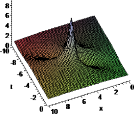
Figure 1. The dynamical evolution of $|{q}^{[1]}_{rw}|^{2}$ with specific parameters $K_{0}=1,J_{0}=L_{0}=10,a=1,c=-1$.

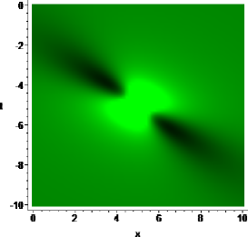
Figure 2. Contour plot of the wave amplitudes of $|{q}^{[1]}_{rw}|^{2}$ for the values used in Figure 1.

Substituting eigenfunctions eq.(53) into eqs.(40), we can get the first order rogue wave ${q}^{[1]}_{rw}$ in the form of determinant. The dynamical evolution of ${q}^{[1]}_{rw}$ for the parametric choice $K_{0}=1,J_{0}=L_{0}=10$ is plotted in the Figure 1, which control the position of the first-order rogue wave by choosing the parameters $K_{0},J_{0}$ and $L_{0}$. Similarly, the corresponding density plot is portrayed in the Figure 2. Theorem 3. For the n-fold DT, the n-order rogue wave ${q}^{[n]}_{rw}$ is of the form

$$q_{rw}^{[n]}=q+\dfrac{\Omega_{r-(n-1)}}{W_{rn}}.$$ (54)

with

$$W_{rn}=\begin{vmatrix}h_{n1}^{1}&h_{n-12}^{1}&h_{n-21}^{1}&h_{n-32}^{1}&\ldots&h_{-(n-2)1}^{1}&h_{-(n-1)2}^{1}\\ {h_{n2}^{1}}^{*}&{h_{n-11}^{1}}^{*}&{h_{n-22}^{1}}^{*}&{h_{n-31}^{1}}^{*}&\ldots&{h_{-(n-2)2}^{1}}^{*}&{h_{-(n-1)1}^{1}}^{*}\\ \vdots&\vdots&\vdots&\vdots&\vdots&\vdots&\vdots\\ h_{n1}^{n}&h_{n-12}^{n}&h_{n-21}^{n}&h_{n-32}^{n}&\ldots&h_{-(n-2)1}^{n}&h_{-(n-1)2}^{n}\\ {h_{n2}^{n}}^{*}&{h_{n-11}^{n}}^{*}&{h_{n-22}^{n}}^{*}&{h_{n-31}^{n}}^{*}&\ldots&{h_{-(n-2)2}^{n}}^{*}&{h_{-(n-1)1}^{n}}^{*}\\ \end{vmatrix},$$

$$\Omega_{r-(n-1)}=\begin{vmatrix}h_{n1}^{1}&h_{n-12}^{1}&h_{n-21}^{1}&h_{n-32}^{1}&\ldots&h_{-(n-2)1}^{1}&-h_{-n1}^{1}\\ {h_{n2}^{1}}^{*}&{h_{n-11}^{1}}^{*}&{h_{n-22}^{1}}^{*}&{h_{n-31}^{1}}^{*}&\ldots&{h_{-(n-2)2}^{1}}^{*}&-{h_{-n2}^{1}}^{*}\\ \vdots&\vdots&\vdots&\vdots&\vdots&\vdots&\vdots\\ h_{n1}^{n}&h_{n-12}^{n}&h_{n-21}^{n}&h_{n-32}^{n}&\ldots&h_{-(n-2)1}^{n}&-h_{-n1}^{n}\\ {h_{n2}^{n}}^{*}&{h_{n-11}^{n}}^{*}&{h_{n-22}^{n}}^{*}&{h_{n-31}^{n}}^{*}&\ldots&{h_{-(n-2)2}^{n}}^{*}&-{h_{-n2}^{n}}^{*}\\ \end{vmatrix},$$

The final form of $\bar{T}_{rn}(\lambda)$ has the form,

$$T_{rn}=T_{rn}(\lambda;\lambda_{1},\lambda_{2},\cdots,\lambda_{2n})=\left(\begin{array}[]{cc}\dfrac{\widetilde{(T_{rn})_{11}}}{W_{rn}}&\dfrac{\widetilde{(T_{rn})_{12}}}{W_{rn}}\\ \\ \dfrac{\widetilde{(T_{rn})_{21}}}{\widetilde{W_{rn}}}&\dfrac{\widetilde{(T_{rn})_{22}}}{\widetilde{W_{rn}}}\\ \end{array}\right),$$ (55)

with

$$\widetilde{(T_{rn})_{11}}=\begin{vmatrix}\lambda^{n}&0&\lambda^{n-2}&0&\ldots&\lambda^{-(n-2)}&0&\lambda^{-n}\\ h_{n1}^{1}&h_{n-12}^{1}&h_{n-21}^{1}&h_{n-32}^{1}&\ldots&h_{-(n-2)1}^{1}&h_{-(n-1)2}^{1}&h_{-n1}^{1}\\ {h_{n2}^{1}}^{*}&{h_{n-11}^{1}}^{*}&{h_{n-22}^{1}}^{*}&{h_{n-31}^{1}}^{*}&\ldots&{h_{-(n-2)2}^{1}}^{*}&{h_{-(n-1)1}^{1}}^{*}&{h_{-n2}^{1}}^{*}\\ \vdots&\vdots&\vdots&\vdots&\vdots&\vdots&\vdots&\vdots\\ h_{n1}^{n}&h_{n-12}^{n}&h_{n-21}^{n}&h_{n-32}^{n}&\ldots&h_{-(n-2)1}^{n}&h_{-(n-1)2}^{n}&h_{-n1}^{n}\\ {h_{n2}^{n}}^{*}&{h_{n-11}^{n}}^{*}&{h_{n-22}^{n}}^{*}&{h_{n-31}^{n}}^{*}&\ldots&{h_{-(n-2)2}^{n}}^{*}&{h_{-(n-1)1}^{n}}^{*}&{h_{-n2}^{n}}^{*}\\ \end{vmatrix},$$

$$\widetilde{(T_{rn})_{12}}=\begin{vmatrix}0&\lambda^{n-1}&0&\lambda^{n-3}&\ldots&0&\lambda^{-(n-1)}&0\\ h_{n1}^{1}&h_{n-12}^{1}&h_{n-21}^{1}&h_{n-32}^{1}&\ldots&h_{-(n-2)1}^{1}&h_{-(n-1)2}^{1}&h_{-n1}^{1}\\ {h_{n2}^{1}}^{*}&{h_{n-11}^{1}}^{*}&{h_{n-22}^{1}}^{*}&{h_{n-31}^{1}}^{*}&\ldots&{h_{-(n-2)2}^{1}}^{*}&{h_{-(n-1)1}^{1}}^{*}&{h_{-n2}^{1}}^{*}\\ \vdots&\vdots&\vdots&\vdots&\vdots&\vdots&\vdots&\vdots\\ h_{n1}^{n}&h_{n-12}^{n}&h_{n-21}^{n}&h_{n-32}^{n}&\ldots&h_{-(n-2)1}^{n}&h_{-(n-1)2}^{n}&h_{-n1}^{n}\\ {h_{n2}^{n}}^{*}&{h_{n-11}^{n}}^{*}&{h_{n-22}^{n}}^{*}&{h_{n-31}^{n}}^{*}&\ldots&{h_{-(n-2)2}^{n}}^{*}&{h_{-(n-1)1}^{n}}^{*}&{h_{-n2}^{n}}^{*}\\ \end{vmatrix},$$

$$\widetilde{(T_{rn})_{21}}=\begin{vmatrix}0&\lambda^{n-1}&0&\lambda^{n-3}&\ldots&0&\lambda^{-(n-1)}&0\\ h_{n2}^{1}&h_{n-11}^{1}&h_{n-22}^{1}&h_{n-31}^{1}&\ldots&h_{-(n-2)2}^{1}&h_{-(n-1)1}^{1}&h_{-n2}^{1}\\ {h_{n1}^{1}}^{*}&{h_{n-12}^{1}}^{*}&{h_{n-21}^{1}}^{*}&{h_{n-32}^{1}}^{*}&\ldots&{h_{-(n-2)1}^{1}}^{*}&{h_{-(n-1)2}^{1}}^{*}&{h_{-n1}^{1}}^{*}\\ \vdots&\vdots&\vdots&\vdots&\vdots&\vdots&\vdots&\vdots\\ h_{n2}^{n}&h_{n-11}^{n}&h_{n-22}^{n}&h_{n-31}^{n}&\ldots&h_{-(n-2)2}^{n}&h_{-(n-1)1}^{n}&h_{-n2}^{n}\\ {h_{n1}^{n}}^{*}&{h_{n-12}^{n}}^{*}&{h_{n-21}^{n}}^{*}&{h_{n-32}^{n}}^{*}&\ldots&{h_{-(n-2)1}^{n}}^{*}&{h_{-(n-1)2}^{n}}^{*}&{h_{-n1}^{n}}^{*}\\ \end{vmatrix},$$

$$\widetilde{(T_{rn})_{22}}=\begin{vmatrix}\lambda^{n}&0&\lambda^{n-2}&0&\ldots&\lambda^{-(n-2)}&0&\lambda^{-n}\\ h_{n2}^{1}&h_{n-11}^{1}&h_{n-22}^{1}&h_{n-31}^{1}&\ldots&h_{-(n-2)2}^{1}&h_{-(n-1)1}^{1}&h_{-n2}^{1}\\ {h_{n1}^{1}}^{*}&{h_{n-12}^{1}}^{*}&{h_{n-21}^{1}}^{*}&{h_{n-32}^{1}}^{*}&\ldots&{h_{-(n-2)1}^{1}}^{*}&{h_{-(n-1)2}^{1}}^{*}&{h_{-n1}^{1}}^{*}\\ \vdots&\vdots&\vdots&\vdots&\vdots&\vdots&\vdots&\vdots\\ h_{n2}^{n}&h_{n-11}^{n}&h_{n-22}^{n}&h_{n-31}^{n}&\ldots&h_{-(n-2)2}^{n}&h_{-(n-1)1}^{n}&h_{-n2}^{n}\\ {h_{n1}^{n}}^{*}&{h_{n-12}^{n}}^{*}&{h_{n-21}^{n}}^{*}&{h_{n-32}^{n}}^{*}&\ldots&{h_{-(n-2)1}^{n}}^{*}&{h_{-(n-1)2}^{n}}^{*}&{h_{-n1}^{n}}^{*}\\ \end{vmatrix},$$

Here

$$h_{m1}^{l}=\dfrac{\partial^{l}}{\partial{\delta}^{l}}((\lambda_{0}+\delta)^{m}\phi_{1}(\lambda_{1}=\lambda_{0}+\delta))|_{\delta=0},m=-n,-(n-1),\cdots,-1,0,1,\cdots,n-1,n,l=1,2,\cdots 2n.$$

$$h_{m2}^{l}=\dfrac{\partial^{l}}{\partial{\delta}^{l}}((\lambda_{0}+\delta)^{m}\varphi_{1}(\lambda_{1}=\lambda_{0}+\delta))|_{\delta=0},m=-n,-(n-1),\cdots,-1,0,1,\cdots,n-1,n,l=1,2,\cdots 2n.$$

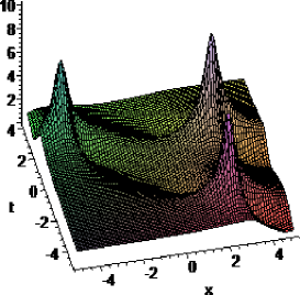
Figure 3. The dynamical evolution of $|{q}^{[2]}_{rw}|^{2}$ with specific parameters $K_{0}=1,J_{0}=-L_{0},J_{1}=L_{1},L_{0}=-5,L_{1}=20,a=1,c=-1$.

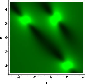
Figure 4. Contour plot of the wave amplitudes of $|{q}^{[2]}_{rw}|^{2}$ for the values used in Figure 3.

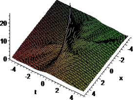
Figure 5. The dynamical evolution of $|{q}^{[2]}_{rw}|^{2}$ with specific parameters $J_{0}=-L_{0},J_{1}=-L_{1},a=1,c=-1$.

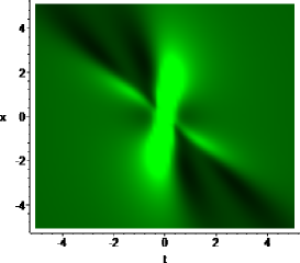
Figure 6. Contour plot of the wave amplitudes of $|{q}^{[2]}_{rw}|^{2}$ for the values used in Figure 5.

Case 1). When $n=2$, substituting eq.(46) into eq.(54), one can construct the second-order rogue waves with seven free parameters. Note that under the condition $J_{1}>>J_{0}$ and $L_{1}>>L_{0}$ except for $J_{0}=-L_{0},J_{1}=-L_{1}$, the second-rogue can split into three first-order rogue wave (triplets rogue wave) [41] rather than two. The dynamical evolution of $|{q}^{[2]}_{rw}|^{2}$ for the parametric choice $K_{0}=1,J_{0}=-L_{0},J_{1}=L_{1},L_{0}=-5,L_{1}=20,a=1,c=-1$ is plotted in the Figure. 3 and the corresponding density plot is shown in the Figure. 4. There is another kind second-order rogue wave, for example, $|{q}^{[2]}_{rw}|^{2}$ is higher than second-rogue above, which is a a fundamental pattern[22]. The dynamical evolution of $|{q}^{[2]}_{rw}|^{2}$ for the parametric choice $J_{0}=-L_{0},J_{1}=-L_{1},a=1,c=-1$ is plotted in the Figure. 5 and the corresponding density map is portrayed in Figure. 6. Note that $|{q}^{[2]}_{rw}|^{2}$ has only two free parameters $a$ and $c$ under the condition $J_{0}=-L_{0},J_{1}=-L_{1}$.

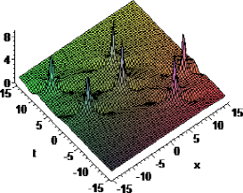
Figure 7. The dynamical evolution of $|{q}^{[3]}_{rw}|^{2}$ with specific parameters $K_{0}=1,J_{0}=-L_{0},J_{1}=-L_{1},J_{2}=L_{2},L_{0}=5,L_{1}=5,L_{2}=3000,a=1,c=-1$.

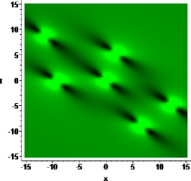
Figure 8. Contour plot of the wave amplitudes of $|{q}^{[3]}_{rw}|^{2}$ for the values used in Figure 7.

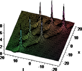
Figure 9. The dynamical evolution of $|{q}^{[3]}_{rw}|^{2}$ with specific parameters $K_{0}=1,J_{0}=-L_{0},J_{1}=L_{1},J_{2}=-L_{2},L_{0}=0,L_{1}=500,L_{2}=0,a=1,c=-1$.

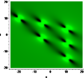
Figure 10. Contour plot of the wave amplitudes of $|{q}^{[3]}_{rw}|^{2}$ for the values used in Figure 9.

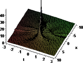
Figure 11. The dynamical evolution of $|{q}^{[3]}_{rw}|^{2}$ with specific parameters $J_{0}=-L_{0},J_{1}=-L_{1},J_{2}=-L_{2},a=1,c=-1$.

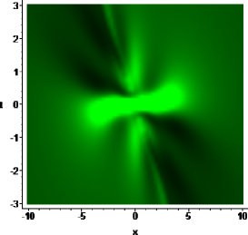
Figure 12. Contour plot of the wave amplitudes of $|{q}^{[3]}_{rw}|^{2}$ for the values used in Figure 11.

Case 2). When $n=3$, substituting eq.(46) into eq.(54) can lead to the third-order rogue waves with nine free parameters. Note that under the condition $J_{2}>>J_{i},L_{2}>>L_{i}(i=0,1)$ or $J_{1}>>J_{i},L_{1}>>L_{i}(i=0,2)$ except for $J_{0}=-L_{0},J_{1}=-L_{1},J_{2}=-L_{2}$, the third-rogue can split into six first-order rogue wave rather. Circular rogue wave [44] may be constructed by the condition $J_{2}>>J_{i},L_{2}>>L_{i}(i=0,1)$ except for $J_{0}=-L_{0},J_{1}=-L_{1},J_{2}=-L_{2}$. The dynamical evolution of $|{q}^{[3]}_{rw}|^{2}$(circular pattern) for the parametric choice $K_{0}=1,J_{0}=-L_{0},J_{1}=-L_{1},J_{2}=L_{2},L_{0}=5,L_{1}=5,L_{2}=3000,a=1,c=-1$ is plotted in the Figure. 7 and the corresponding density plot in Figure. 8. At the same time, triplets rogue wave may be constructed by the condition $J_{1}>>J_{i},L_{1}>>L_{i}(i=0,2)$ except for $J_{0}=-L_{0},J_{1}=-L_{1},J_{2}=-L_{2}$. The dynamical evolution of $|{q}^{[3]}_{rw}|^{2}$(triangular pattern) for the parametric choice $K_{0}=1,J_{0}=-L_{0},J_{1}=L_{1},J_{2}=-L_{2},L_{0}=0,L_{1}=500,L_{2}=0,a=1,c=-1$ is plotted in the Figure. 9 and its density map in Figure. 10. Similarly, there is another kind of third-order rogue wave, for example, $|{q}^{[3]}_{rw}|^{2}$ is higher than third-rogue above. The dynamical evolution of $|{q}^{[3]}_{rw}|^{2}$(fundament pattern) for the parametric choice $J_{0}=-L_{0},J_{1}=-L_{1},J_{2}=-L_{2},a=1,c=-1$ is plotted in the Figure. 11. Similarly, the density plot of Figure. 11 and the corresponding density plot in Figure. 12. Note that $|{q}^{[3]}_{rw}|^{2}$ has only two free parameters $a$ and $c$ under the condition $J_{0}=-L_{0},J_{1}=-L_{1},J_{2}=-L_{2}$.

Case 3). When $n=4$, substituting eq.(46) into eq.(54) one can generate the four-order rogue waves with eleven free parameters. Note that under the condition $J_{3}>>J_{i},L_{3}>>L_{i}(i=0,1,2)$ or $J_{2}>>J_{i},L_{2}>>L_{i}(i=0,1,3)$ or $J_{1}>>J_{i},L_{1}>>L_{i}(i=0,2,3)$ except for $J_{0}=-L_{0},J_{1}=-L_{1},J_{2}=-L_{2},J_{3}=-L_{3}$, the four-rogue waves can split into ten first-order rogue wave rather. One kind of circular rogue wave [44] may be constructed by the condition $J_{3}>>J_{i},L_{3}>>L_{i}(i=0,1,2)$ except for $J_{0}=-L_{0},J_{1}=-L_{1},J_{2}=-L_{2},J_{3}=-L_{3}$. The dynamical evolution of $|{q}^{[4]}_{rw}|^{2}$, which is a fourth order rouge wave consisting of a ring structure (outer,seven peaks) and a fundamental pattern of the second rogue wave (inner), for the parametric choice $K_{0}=1,J_{0}=-L_{0},J_{1}=-L_{1},J_{2}=-L_{2},J_{3}=L_{3},L_{0}=L_{1}=L_{2}=5,L_{3}=2000,a=1,c=-1$ is plotted in the Figure. 13 and the corresponding density plot in Figure. 14. In addition, the dynamical evolution of $|{q}^{[4]}_{rw}|^{2}$, which is another circular pattern rogue wave [44], for the parametric choice $K_{0}=1,J_{0}=L_{0},J_{1}=-L_{1},J_{2}=-L_{2},J_{3}=L_{3},L_{0}=50,L_{1}=10,L_{2}=0,L_{3}=2000,a=1,c=-1$ is plotted in the Figure. 15. and its density map is portrayed in Figure.16. Note that the inner structure of Figure 15 (or 16) is a triangular pattern of a second order rogue wave. At the same time, the triangular pattern of the rogue wave may be constructed by the condition $J_{1}>>J_{i},L_{1}>>L_{i}(i=0,2,3)$ except for $J_{0}=-L_{0},J_{1}=-L_{1},J_{2}=-L_{2},J_{3}=-L_{3}$. The dynamical evolution of $|{q}^{[4]}_{rw}|^{2}$(triangular pattern) for the parametric choice $K_{0}=1,J_{0}=-L_{0},J_{1}=L_{1},J_{2}=-L_{2},J_{3}=-L_{3},L_{0}=0,L_{1}=2000,L_{2}=L_{3}=0,a=1,c=-1$ is plotted in the Figure. 17 and its density plot in Figure. 18. A pentagon pattern of the rogue wave may be constructed by the condition $J_{2}>>J_{i},L_{2}>>L_{i}(i=0,1,3)$ except for $J_{0}=-L_{0},J_{1}=-L_{1},J_{2}=-L_{2},J_{3}=-L_{3}$. The dynamical evolution of $|{q}^{[4]}_{rw}|^{2}$ (pentagon pattern) for the parametric choice $K_{0}=1,J_{0}=-L_{0},J_{1}=-L_{1},J_{2}=L_{2},J_{3}=-L_{3},L_{0}=L_{1}=0,L_{2}=2000,L_{3}=0,a=1,c=-1$ is plotted in the Figure. 19. Similarly, the density plot of Figure. 19 is correspondingly shown in Figure. 20. Similarly, there is another kind four-order rogue wave, for example, $|{q}^{[4]}_{rw}|^{2}$ is higher than four-rogue above. The dynamical evolution of $|{q}^{[4]}_{rw}|^{2}$ (fundamental pattern) for the parametric choice $J_{0}=-L_{0},J_{1}=-L_{1},J_{2}=-L_{2},J_{3}=-L_{3},a=1,c=-1$ is plotted in the Figure. 21 and the corresponding density plot is portrayed in Figure. 22. Note that $|{q}^{[4]}_{rw}|^{2}$ only has two free parameters $a$ and $c$ under the condition $J_{0}=-L_{0},J_{1}=-L_{1},J_{2}=-L_{2},J_{3}=-L_{3}$. According to the above analysis, the n-order rogue waves may be controlled by $2n+3$ free parameters.

4. Conclusions

Thus, in this paper, considering FL system of equation which describes nonlinear pulse propagation through single mode optical fiber, the determinant representation of the N-fold DT for the FL system is given in eqs.(36). The n-order rogue wave in eq.(54) of the FL equation is obtained by this representation from a periodic seed under the reduction condition eq.(41). Several interesting patterns of the rogue wave are plotted by choosing suitable parameters.

Our results provide an alternative possibility to observe rogue waves in optical system. Moreover, from the one-fold DT, it is interesting to observe that the DT of the FL system exhibits the following novelty in comparison with other integrable models like the AKNS and the KN systems: the DT matrix of the FL system has three different terms depending on $\lambda$. Thus, the DT as well as the rogue wave of the FL system holds novel features, in comparison with the DT and rogue wave solutions of the standard integrable counterparts like the AKNS and the KN systems. The n-order rogue waves of the FL equation are constructed by using the determinant representation of the DT with $2n+3$ free parameters.

Acknowledgments This work is supported by the NSF of China under Grant No.10971109 and K.C.Wong Magna Fund in Ningbo University. Jingsong He is also supported by Program for NCET under Grant No.NCET-08-0515 and Natural Science Foundation of Ningbo under Grant No.2011A610179. We thank Prof. Yishen Li(USTC,Hefei, China) for his useful suggestions on the rogue wave. J. He thank Prof. A.S.Fokas (Cambridge University) for many helps on this paper.

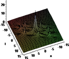
Figure 13. The dynamical evolution of $|{q}^{[4]}_{rw}|^{2}$ with specific parameters $K_{0}=1,J_{0}=-L_{0},J_{1}=-L_{1},J_{2}=-L_{2},J_{3}=L_{3},L_{0}=L_{1}=L_{2}=5,L_{3}=2000,a=1,c=-1$.

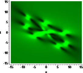
Figure 14. Contour plot of the wave amplitudes of $|{q}^{[4]}_{rw}|^{2}$ for the values used in Figure 13.

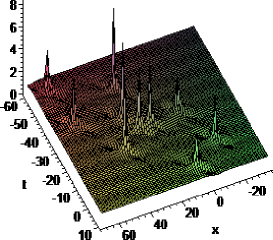
Figure 15. The dynamical evolution of $|{q}^{[4]}_{rw}|^{2}$ with specific parameters $K_{0}=1,J_{0}=L_{0},J_{1}=-L_{1},J_{2}=-L_{2},J_{3}=L_{3},L_{0}=50,L_{1}=10,L_{2}=0,L_{3}=2000,a=1,c=-1$.

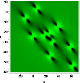
Figure 16. Contour plot of the wave amplitudes of $|{q}^{[4]}_{rw}|^{2}$ for the values used in Figure 15.

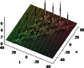
Figure 17. The dynamical evolution of $|{q}^{[4]}_{rw}|^{2}$ with specific parameters $K_{0}=1,J_{0}=-L_{0},J_{1}=L_{1},J_{2}=-L_{2},J_{3}=-L_{3},L_{0}=0,L_{1}=2000,L_{2}=L_{3}=0,a=1,c=-1$.

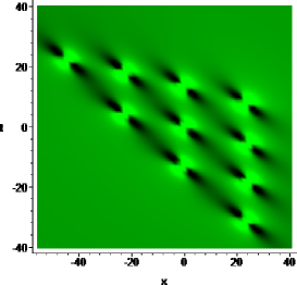
Figure 18. Contour plot of the wave amplitudes of $|{q}^{[4]}_{rw}|^{2}$ for the values used in Figure 17.

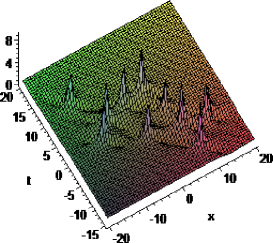
Figure 19. The dynamical evolution of $|{q}^{[4]}_{rw}|^{2}$ with specific parameters $K_{0}=1,J_{0}=-L_{0},J_{1}=-L_{1},J_{2}=L_{2},J_{3}=-L_{3},L_{0}=L_{1}=0,L_{2}=2000,L_{3}=0,a=1,c=-1$.

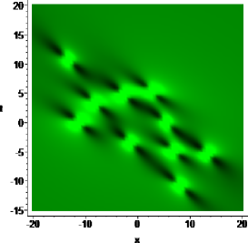
Figure 20. Contour plot of the wave amplitudes of $|{q}^{[4]}_{rw}|^{2}$ for the values used in Figure 19.

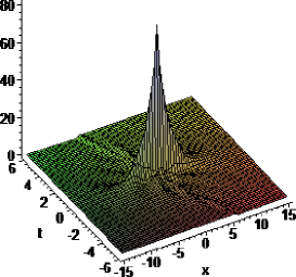
Figure 21. The dynamical evolution of $|{q}^{[4]}_{rw}|^{2}$ with specific parameters $J_{0}=-L_{0},J_{1}=-L_{1},J_{2}=-L_{2},J_{3}=-L_{3},a=1,c=-1$.

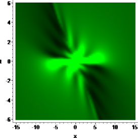
Figure 22. Contour plot of the wave amplitudes of $|{q}^{[4]}_{rw}|^{2}$ for the values used in Figure 21.