Device-Independent Randomness Generation in the Presence of Weak Cross-Talk

Abstract

Device-independent protocols use nonlocality to certify that they are performing properly. This is achieved via Bell experiments on entangled quantum systems, which are kept isolated from one another during the measurements. However, with present-day technology, perfect isolation comes at the price of experimental complexity and extremely low data rates. Here we argue that for device-independent randomness generation – and other device-independent protocols where the devices are in the same lab – we can slightly relax the requirement of perfect isolation, and still retain most of the advantages of the device-independent approach, by allowing a little cross-talk between the devices. This opens up the possibility of using existent experimental systems with high data rates, such as Josephson phase qubits on the same chip, thereby bringing device-independent randomness generation much closer to practical application.

Introduction – The great advantage of device-independent (DI) protocols is their reliance on a small set of tests, which are nevertheless sufficient to certify that they are performing properly. This is achieved by carrying out nonlocality tests on entangled quantum systems. In particular, no assumptions are made regarding the inner workings of the devices, such as the Hilbert space dimension of the underlying quantum systems, etc. Mayers ; Acin . Each device is treated as a ‘black box’ with knobs and registers for selecting and displaying (classical) inputs and outputs. Applications include quantum key-distribution Barrett ; Acin ; McKague ; Masanes ; Reichardt ; Vazirani , coin flipping Silman , state tomography Bardyn ; McKague 3 ; Reichardt , genuine multi-partite entanglement detection Bancal , self-testing of quantum computers Magniez ; McKague 2 , as well as DI randomness generation (RG) Colbeck ; Pironio ; Pironio 2 ; Fehr ; Vazirani 2 .

It is often remarked that DI cryptographic protocols remain secure even if the devices have been provided, or sabotaged, by an adversary. This scenario, while conceptually fascinating, is of little (if any) practical relevance. This is because (i) there are many types of attacks available to a malicious provider – the majority being classical – that eliminating them all is an enormous task; (ii) in any case we assume the existence of honest providers of e.g. the source of randomness, the jamming technology to prevent information leakage from the labs, or the classical devices used to process the data. A scenario where one can trust the latter, but an honest provider for the quantum devices cannot be found, is highly implausible.

The actual advantage of DI protocols is that they allow us to monitor the performance of the devices irrespectively of noise, imperfections, lack of knowledge regarding their inner workings, or limited control over them. Indeed, even if the devices were obtained from a trusted provider and thoroughly inspected, many things can still unintentionally go wrong (as demonstrated by the attacks on commercial quantum key-distribution systems Zhao ; Xu ; Lydersen , which exploited unintentional design flaws).

This problem is particularly acute in the case of DI RG, as it is very difficult even for honest parties to maufacture reliable randomness generators (whether classical or quantum) and monitor them for malfunction. The generation of randomness in a DI manner solves many of the shortcomings of customary RG protocols, since, as mentioned above, the degree of violation of a Bell inequality provides an accurate estimate of the amount of randomness generated irrespectively of experimental imperfections and lack of control. DI RG has so far been proven secure against adversaries with classical side-information about the devices (which is the relevant case when the provider is trusted) for arbitrary Bell inequalities and degrees of violation Pironio 2 ; Fehr , and against adversaries with quantum side-information in the case of very high violation of the CHSH inequality Vazirani 2 .

Unfortunately, DI RG is experimentally highly challenging. It requires a Bell experiment with the detection loophole closed and with the quantum systems isolated from one another.

A proof of principle experiment was reported in Pironio using two ions in separate vacuum traps, but this system operates at an extremely low rate ($\sim 1\,\mathrm{mHz}$), precluding any practical application. Nevertheless, there exist today experiments involving, for example, two Josephson phase qubits on the same chip coupled by a radio frequency resonator Ansmann , or two ions in the same trap coupled via their vibrational modes Rowe ; Monz , which allow for Bell violating experiments (with the detection loophole closed) at much higher data rates ($\gtrsim 1\,\mathrm{kHz}$).

In these experiments the quantum systems are very close to one another. This proximity provides the non-negligible coupling required for high entanglement generation rates. Adapting DI RG to these types of experiments would bring it much closer to real-life application. The problem is that precisely because the systems are close to one another and non-negligibly coupled, they can no longer be considered as completely isolated (see Martinis and Haffner for a discussion of the couplings involved). The aim of the present work is to show how to take this coupling into account by relaxing slightly the assumptions behind the DI approach, while keeping as much as possible all of its advantages.

We begin by showing how to derive bounds on the RG rate in a DI setting given a known amount of cross-talk (CT). Next, we present methods for estimating the amount of CT present in an experiment. Our approach is then illustrated on Josephson phase qubits, showing that efficient DI RG is possible using already established technology. We start first, however, by recalling briefly the essential ingredients of DI RG relevant to our analysis. We refer to Pironio ; Pironio 2 ; Fehr for a more detailed presentation.

Bell inequalities and device-independent randomness generation – A Bell experiment is characterized by the probabilities $\mathcal{P}=\left\{P_{ab\mid xy}\right\}$ of obtaining the outcomes (or outputs) $a$ and $b$ given the measurement settings (or inputs) $x$ and $y$. A Bell expression $\mathcal{I}\left(\mathcal{P}\right)=\sum_{abxy}c_{abxy}P_{ab|xy}$ is a linear function of these probabilities. For instance, the CHSH inequality has the form $\mathcal{I}\left(\mathcal{P}\right)=\sum_{a,\,b,\,x,\,y\in\left\{0,\,1\right\}}\left(-1\right)^{a\oplus b\oplus xy}P_{ab\mid xy}\leq 2$. To any Bell expression, one can associate a bound on the randomness of the outputs given the inputs $x$ and $y$ through a function $P_{xy}^{*}\left(I\right)$ such that $\max_{a,\,b}P_{ab\mid xy}\leq P_{xy}^{*}\left(I\right)$ holds for any $\mathcal{P}$ for which $\mathcal{I}\left(\mathcal{P}\right)=I$ Pironio ; Pironio 2 ; Fehr . The function $P_{xy}^{*}\left(I\right)$ should be monotonically decreasing and concave in $I$ (if not we can take its concave hull). Higher values of $P_{xy}^{*}(I)$ imply less randomness, in particular when $\min_{x,\,y}P_{xy}^{*}(I)=1$ the system is fully deterministic.

Given knowledge of such a function and the degree of Bell violation $I$ observed in an experiment where the devices are used $n$ times in succession, one can infer a lower bound on the min-entropy of the measurement outcomes. By applying a randomness extractor to the resulting string of outcomes, one then obtains a new private string of random numbers of length $\simeq-n\log_{2}P^{*}_{xy}(I)$ which is arbitrarily close (up to a security parameter) to the uniform distribution. Depending on the assumptions made regarding the devices and the adversary, such a protocol may also require an initial random seed (in which case one talks about DI randomness expansion) that may be polynomially Pironio or exponentially Pironio 2 ; Fehr smaller than the output string.

Device-independent randomness generation with weak cross-talk – In the security analysis of DI RG protocols the assumption that the two Bell violating devices are isolated from one another only appears in the derivation of the bound $P_{xy}^{*}\left(I\right)\geq\max_{a,\,b}P_{ab\mid xy}$. If we introduce a similar bound $P_{xy}^{*}\left(I,\chi\right)$ that is valid in the presence of a given amount of CT $\chi$ (defined below), then the rest of the reasoning of Pironio ; Pironio 2 ; Fehr will apply without modification.

To define such a CT-dependent bound, we write the probabilities observed in a Bell experiment as $P_{ab|xy}=\mathrm{Tr}\left(\rho\Pi_{ab|xy}\right)$, where $\rho\in\mathcal{H}_{A}\otimes\mathcal{H}_{B}$ and $\{\Pi_{ab|xy}\}$ is a POVM on $\mathcal{H}_{A}\otimes\mathcal{H}_{B}$ (i.e. $\Pi_{ab|xy}\succeq 0$ and $\sum_{ab}\Pi_{ab|xy}=\mathds{1}$). The novelty with respect to the standard mathematical description of Bell experiments is in allowing the measurement $\Pi_{ab|xy}$ to act collectively on the two systems. We will say that such a collective measurement requires no more than $\chi$ amount of CT if there exists a product POVM $\{\Pi_{a|x}\otimes\Pi_{b|y}\}$ satisfying

$$-\chi\mathds{1}\preceq\Pi_{ab|xy}-\Pi_{a|x}\otimes\Pi_{b|y}\preceq\chi\mathds{1}$$ (1)

for all combinations of $a$ and $b$. This condition restricts how far each collective POVM may be from a product of two independent POVMs. In particular, when $\chi=0$ the $\Pi_{ab|xy}$ can be expressed as products, while when $\chi=1$ they are unconstrained.

Consider now a fixed value of $\chi$ and a Bell violation $I$. Then the solution of the following program provides the minimal amount of randomness $P^{*}_{xy}(I,\chi)$ compatible with $I$ and $\chi$:

$$P_{xy}^{*}(I,\chi)=\max_{a,\,b}\max_{Q}\quad P_{ab\mid xy}$$ (2)

$$\mathrm{s.t.}\quad P_{ab\mid xy}=\mathrm{Tr}\left(\rho\Pi_{ab|xy}\right),\quad\mathcal{I}\left(\mathcal{P}\right)=I,$$

$$-\chi\mathds{1}\preceq\Pi_{ab|xy}-\Pi_{a|x}\otimes\Pi_{b|y}\preceq\chi\mathds{1}\,,$$

where the optimization runs over the set $Q=\{\rho,\,\{\Pi_{a|x}\},\,\{\Pi_{b|y}\},\,\{\Pi_{ab|xy}\},\,\mathcal{H}_{A},\,\mathcal{H}_{B}\}$ specifying the state, measurements, and the Hilbert spaces. This formulation is therefore DI in spirit, since the bound is formulated without fixing the dimension of the Hilbert spaces, nor how the measurements are implemented, etc.

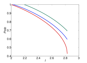
Figure 1: DI upper bounds on $P^{*}_{00}$. The middle (top) curve gives an SDP based upper bound obtained from Eq. (2) (Eq. (3)), as a function of the CHSH violation $I$, given $\chi=0.01$. The bottom curve bounds $P^{*}_{00}$ when $\chi=0$.

Upper bounds on the optimization problem Eq. (2) can be obtained using the techniques of Navascues ; Pironio 3 , which relax the problem to a hierarchy of semi-definite programs (SDPs). In particular, the resulting series of bounds is guaranteed to converge to the true solution. Nevertheless, depending on the problem, even the lowest order relaxation may be computationally intractable. We may then obtain a weaker bound in terms of $P_{xy}^{*}\left(I,\,0\right)$ – the solution in the absence of CT. Let $\rho^{\prime}$, $\{\Pi_{a|x}^{\prime}\}$, $\{\Pi_{b|y}^{\prime}\}$, and $\{\Pi_{ab|xy}^{\prime}\}$ be the state and POVMs corresponding to the solution of Eq. (2), and let $P^{\prime}_{ab\mid xy}=\mathrm{Tr}(\rho^{\prime}\Pi_{a|x}^{\prime}\otimes\Pi_{b|y}^{\prime})$ and $\mathcal{P}^{\prime}=\{P^{\prime}_{ab|xy}\}$. From the last constraint in Eq. (2) we have that $|P_{ab\mid xy}-P^{\prime}_{ab\mid xy}|\leq\chi$, and so $\mathcal{I}(\mathcal{P}^{\prime})\geq\mathcal{I}(\mathcal{P})-\gamma\chi$ where $\gamma=\sum_{a,\,b,\,x,\,y}\left|c_{abxy}\right|$ (in the case of the CHSH inequality for instance $\gamma=16$). Taken together, the last two inequalities imply that

$$P_{xy}^{*}\left(I,\,\chi\right)\leq P_{xy}^{*}\left(I-\gamma\chi,\,0\right)+\chi\,.$$ (3)

Fig. 1 displays upper bounds on $P_{00}^{*}$ obtained from Eq. (2) and Eq. (3) in the case of the CHSH inequality.

Finally, we note that the last constraint in Eq. (2) implies that the signaling – the extent to which the output of one device depends on the input of the other – is constrained. Specifically, if to each input $x$ and each input $y$ correspond $N$ outputs, $|P_{a|xy}-P_{a|xy^{\prime}}|\leq 2N\chi$ for all $a,\,x,\,y,\,y^{\prime}$, etc. (in the case of zero signaling, one has $P_{a|xy}=P_{a|xy^{\prime}}$). This allows us to derive a simpler bound on $P^{*}_{xy}$, depending solely on the amount of signaling present, in contrast to the bounds Eqs. (2) and (3), which rely on the full structure of quantum mechanics. To this end we define the maximal amount of signaling allowed as

$$\delta=\max\Bigl{\{}\max_{a,\,x,\,y,\,y^{\prime}}|P_{a|xy}-P_{a|xy^{\prime}}|,\,\max_{b,\,y,\,x,\,x^{\prime}}|P_{b|xy}-P_{b|x^{\prime}y}|\Bigr{\}}\,.$$ (4)

When $\delta=0$, $\mathcal{P}$ resides within the no-signaling polytope Barrett 2 , while when $\delta>0$ $\mathcal{P}$ resides within a larger, higher-dimensional polytope. The bound can be obtained by solving the linear program $P^{*}_{xy}(I,\,\delta)=\max_{ab}P_{ab|xy}$, given that $I(\mathcal{P})=I$, $|P_{a|xy}-P_{a|xy^{\prime}}|\leq\delta$, and $|P_{b|xy}-P_{b|x^{\prime}y}|\leq\delta$. In the case of the CHSH inequality, one can show that (see Appendix A)

$$P^{*}_{xy}(I,\delta)\leq\frac{3}{2}-\frac{1}{4}I+2\delta\,.$$ (5)

This bound applies to any post-quantum theory which restricts the amount of signaling (as well as to quantum mechanics).

Estimating the amount of cross-talk – We have just seen how the introduction of a new security parameter $\chi$, quantifying the amount of CT between the devices, allows us to extend the scope of DI RG to settings with a limited amount of CT. To apply this approach, we therefore need a reliable prior estimate of $\chi$, and means of guaranteeing or verifying that the CT will not exceed this estimate during latter operations of the devices. This obviously requires some modeling of the devices’ inner workings. Indeed, it is impossible to upper-bound the amount of CT from first principles only or from any set of observed data $\mathcal{P}$ alone, since communicating devices can deterministically reproduce any $\mathcal{P}$, and therefore simulate any degree of Bell violation.

At first, this may seem an unwelcome departure from the purely DI approach (i.e. $\chi=0$). Nevertheless, our approach has the advantage over fully device-dependent approaches that only a single parameter $\chi$ must be device-dependently estimated to ensure that the protocol performs properly, and this same parameter is used irrespectively of the underlying physical realization. Morever, even in purely DI protocols the absence of communication cannot be deduced from the observed data alone, and to verify that there is indeed no-communication will necessarily involve putting our trust in certain general assumptions regarding the behavior of the devices, or relying on some trusted external hardware. Seen in this light, our approach is not very different from the standard (DI) one, except that instead of verifying in some trusted way that $\chi=0$, we must verify that $\chi$ is no greater than some finite value. Finally, we note that our approach allows as a safeguard to set $\chi$ to be greater than its expected value – a feature that may be useful even in for purely DI protocols with (allegedly) non-communicating devices.

Even though a maximal amount of CT $\chi$ cannot be guaranteed without some modeling of the devices, there are several ways to lower-bound $\chi$ from the observed data $\mathcal{P}$ only. If the devices were not fabricated by an adversary and do not act maliciously, then these lower bounds may provide good estimates of $\chi$.

A simple way to lower-bound $\chi$ in a DI manner is via the degree of violation of the no-signaling conditions Eq. (4), computed from the observed data $\mathcal{P}$. From Eq. (4) it follows that $\chi\geq\delta/2N$. Improved DI bounds are obtainable, however, reflecting the fact that $\delta$ does not capture all of the information contained in $\mathcal{P}$. The minimal amount of CT that is compatible with a given $\mathcal{P}$ is given by the solution of the following optimization problem

$$\min_{\mathcal{Q}}\quad\chi$$ (6)

$$\mathrm{s.t.}\quad\mathrm{Tr}\left(\rho\Pi_{ab|xy}\right)=P_{ab\mid xy},$$

$$-\chi\mathds{1}\preceq\Pi_{ab|xy}-\Pi_{a|x}\otimes\Pi_{b|y}\preceq\chi\mathds{1},$$

which can be lower-bounded using the techniques of Navascues ; Pironio 3 . It is clear that this bound is optimal, since the optimization runs over all possible states $\rho$ and sets of projectors $\{\Pi_{a|x}\}$, $\{\Pi_{b|y}\}$ and $\{\Pi_{ab|xy}\}$ satisfying the constraints in Eq. (2). That it constitutes an improvement over the bound provided by Eq. (4) is seen by considering the case of post-quantum non-signaling distributions (including those that do not violate Tsirelson’s bound Tsirelson ). Such distributions will not give rise to a non-vanishing bound via Eq. (4). However, since they cannot be realized quantumly without communication, they will give rise to a non-vanishing bound via Eq. (6). See Fig. 2.

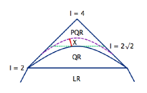
Figure 2: Part of the no-signaling polytope. The curved solid line separates the post-quantum region (PQR) from the quantum region (QR) – the set of probabilities that can be realized by product measurements on quantum states. The straight dashed line represents Tsirelson’s bound. The horizontal solid line separates QR from the classical or local region (LR). The top vertex corresponds to the PR box Popescu . Although non-signaling, points in PQR cannot be realized by product measurements, but only by non-product ones. Restricting the amount of CT to $\chi$, only points below the curved dahsed line are (quantumly) realizable.

It is possible of course that the true value of $\chi$ is not revealed by the above lower bounds (for instance, points in QR in Fig. 2 can be reproduced either with or without CT and thus the real value of $\chi$ cannot be unambiguously determined from the observed data $\mathcal{P}$ alone). Nevertheless, one can also adopt a more device-dependent approach to estimating $\chi$. In particular, if the lower bound provided by Eq. (6) equals zero, one can vary the state and the measurements. Such a procedure could in principle reveal the presence of any fixed interaction Hamiltonian $H$, since it has been shown that for any such interaction there exists a strategy involving only local operations and classical communication that reveals the presence of the interaction as signaling Bennett . However, we do not know of any systematic way for finding this strategy if $H$ is unknown, nor do we know how to relate in a systematic way the observed signaling to $H$.

Finally, by modeling the physical systems, their interaction and the measurement procedure, it is possible to estimate the amount of CT. An example of this last approach are given below.

Candidates for real-life implementation – A system ideally suited for the implemenation of DI RG will (i) give rise to a sufficiently high Bell violation with the detection loophole kept closed, (ii) exhibit a negligible amount of CT, and (iii) allow for very high data rates. We discuss below an experiment based on Josephson phase qubits, which meets all of these requirements. Another possibility is based on trapped ions, as discussed in Appendix B.

In the CHSH experiment of Ansmann two Josephson phase qubits, coupled by a radio frequency strip resonator, are used. The qubits are located on the same chip, separated by $3.1\,\mathrm{mm}$, and are entangled by successively coupling them to the strip resonator. Single qubit rotations are effected by applying microwaves at the resonance frequency of the corresponding qubit. Read-out is effected by letting the excited state tunnel to an auxiliary state macroscopically distinct from both the ground state and the excited state. All operations can be carried out on time scales significantly shorter than $1\,\mu\mathrm{s}$. (For a recent review of Josephson phase qubits experiments see Martinis .)

The constant coupling between the qubits gives rise to some CT. From the analysis of the experimental set up performed in Ansmann and Kofman , it appears that the most significant contribution to the CT occurs during the read-out: The tunneling of one qubit from the excited state to a macroscopically distinct state sometimes forces the other qubit to tunnel when in the ground state. This allows us to estimate the CT at $0.0030$ (see Appendix C). The same value is also obtained by solving the second order relaxation of Eq. (6) using the set of observed data found in in the Supplementary Information for Ansmann .

For the reported degree of CHSH violation $I=2.0732$, and the above value of the CT, we find that $P_{00}^{*}\leq 0.983$. To establish robustness we note that for as a low a violation as $I=2.002$ $P_{00}^{*}\leq 0.998$. This shows that useful randomness is extractable from this experiment.

Conclusion – The analysis of any DI protocol requires that we specify the amount of CT between the devices (irrespectively of whether it is vanishing or finite) – a requirement that cannot be fully verified or implemented in a DI manner. In this work we have shown that one can relax the maxims appearing previous works on DI RG, by allowing for a small amount of CT between the quantum systems. In this way we can keep most of the advantages of the DI approach and at the same time reach data rates of practical interest. Finally, we note that our approach can be generalized to other DI protocols where the devices are in the same lab, such as DI tests of genuine multi-partite entanglement Bancal .

Appendix A

We prove here Eq. (5). Eq. (5) can be re-expressed as $4P^{*}_{xy}(I,\,\delta)\geq\left(4-I\right)+\left(2+8\delta\right)$. The first term on the right-hand side is now seen to be a sum of probabilities, all of which appear in the CHSH inequality with a minus sign:

$$4-I=\sum_{a,\,b,\,x,\,y}\left[1-(-1)^{a\oplus b\oplus xy}\right]P_{ab\mid xy}$$

$$=2\sum_{a}\left(P_{a\bar{a}\mid 00}+P_{a\bar{a}\mid 01}+P_{a\bar{a}\mid 10}+P_{aa\mid 11}\right)\,,$$ (7)

where $\bar{a}=a\oplus 1$. Hence, any probability, appearing in the CHSH inequality with a negative sign, is smaller or equal to $2-I/2$.

Consider now the following relation

$$2+8\delta\geq 2+2\sum_{x,\,y}\left[\left(-1\right)^{y}P_{a\mid xy}+\left(-1\right)^{x}P_{b\mid xy}\right]$$

$$=2+2\bigl{(}2P_{ab\mid 00}+P_{a\bar{b}\mid 00}-P_{a\bar{b}\mid 01}+P_{a\bar{b}\mid 10}-2P_{ab\mid 11}-P_{a\bar{b}\mid 11}+P_{\bar{a}b\mid 00}-P_{\bar{a}b\mid 10}+P_{\bar{a}b\mid 01}-P_{\bar{a}b\mid 11}\bigr{)}$$

$$\geq 2+2\bigl{(}2P_{ab\mid 00}-P_{a\bar{b}\mid 01}-2P_{ab\mid 11}-P_{a\bar{b}\mid 11}-P_{\bar{a}b\mid 10}-P_{\bar{a}b\mid 11}\bigr{)}$$ (8)

$$\geq 2+2\bigl{(}2P_{ab\mid 00}-P_{a\bar{b}\mid 01}-P_{ab\mid 11}-1+P_{\bar{a}\bar{b}\mid 11}-P_{\bar{a}b\mid 10}\bigr{)}$$

$$\geq 2\bigl{(}2P_{ab\mid 00}-P_{a\bar{b}\mid 01}-P_{ab\mid 11}-P_{\bar{a}b\mid 10}\bigr{)}\,.$$

Setting $b=a$ and summing $4-I$ and $2+8\delta$, we get

$$6-I+8\delta\geq 4P_{aa\mid 00}+2\left(P_{a\bar{a}\mid 00}+P_{\bar{a}a\mid 00}+P_{\bar{a}a\mid 01}\right.$$

$$\left.+P_{a\bar{a}\mid 10}+P_{\bar{a}\bar{a}\mid 11}\right)\,,$$ (9)

and so

$$P_{aa\mid 00}\leq\frac{3}{2}-\frac{1}{4}I+2\delta\,.$$ (10)

Similarly, from

$$4\delta\geq\sum_{x,\,y}\bigl{[}\left(-1\right)^{x+y+1}P_{a\mid xy}+\left(-1\right)^{x}P_{b\mid xy}\bigr{]}\,,$$ (11)

it follows that

$$P_{aa\mid 01}\leq\frac{3}{2}-\frac{1}{4}I+2\delta\,,$$ (12)

from

$$4\delta\geq\sum_{x,\,y}\bigl{[}\left(-1\right)^{y}P_{a\mid xy}+\left(-1\right)^{x+y+1}P_{b\mid xy}\bigr{]}$$ (13)

it follows that

$$P_{aa\mid 10}\leq\frac{3}{2}-\frac{1}{4}I+2\delta\,,$$ (14)

and from

$$4\delta\geq\sum_{x}\Bigl{[}\sum_{y}\left(-1\right)^{x+y}P_{a\mid xy}+\left(-1\right)^{x+1}\bigl{(}P_{b\mid x0}+P_{\bar{b}\mid x1}\bigr{)}\Bigr{]}$$ (15)

it follows that

$$P_{a\bar{a}\mid 11}\leq\frac{3}{2}-\frac{1}{4}I+2\delta\,,$$ (16)

and so any probability appearing in the CHSH inequality with a positive sign is smaller or equal to $\frac{3}{2}-\frac{1}{4}I+2\delta$. We therefore have that whenever $I\geq 2$ (the case $I\leq 2$ being trivial)

$$P^{*}_{xy}(I,\,\delta)\leq\max\Bigl{\{}2-\frac{1}{2}I,\,\frac{3}{2}-\frac{1}{4}I+2\delta\Bigr{\}}=\frac{3}{2}-\frac{1}{4}I+2\delta\,$$ (17)

for all pairs of inputs $x$ and $y$.

Appendix B

We derive here a rough estimate for the amount of CT present in the experiments such as Monz . Vibrationally coupled ions in the same trap are one of the most advanced quantum information processing systems. The system is initialized by preparing the ions in their vibrational ground state, following which they are entangled via the vibrational coupling. Measurements can be realized on each ion individually: First, to choose the measurement setting, single qubit gate operations are performed by addressing the ions individually with focused light beams. The state of each ion is then measured in the computational basis using fluorescence. The whole process takes $\lesssim 1\,\mathrm{ms}$ and the fidelities of the gates and measurements are high ($\sim 99\,\%$). (For a recent review of quantum information processing using ion traps see Haffner .)

In these experiments the ions are typically separated by $\sim 5\,\mu\mathrm{m}$, resulting in some CT. It seems that the main contribution to the CT is due to the single qubit rotations performed to select the measurement settings. Indeed, the light beams used to address the ions have a width of $2\,\mu\mathrm{m}$. As a result, if the state of one ion is rotated by $\theta$ on the Bloch sphere, the neighbouring ion will be rotated by $\varepsilon\simeq 0.03\theta$ (this is the ratio of Rabi frequencies, as discussed in Haffner ). More specifically, with no loss of generality we may assume that the ideal entangled state shared by the parties is such that the corresponding ideal measurements are projectors onto the states $\left|\psi_{abxy}\right\rangle=\left|a_{\varphi_{x}}\right\rangle\otimes|b_{\varphi_{y}}\rangle$, where $\left|a_{\varphi_{x}}\right\rangle$ ($|b_{\varphi_{y}}\rangle$) denotes a state on the Bloch sphere parametrized by $\theta=\pi/2$ and $\varphi=\varphi_{x}=\left(-1\right)^{x}\pi/4$ ($\varphi=\varphi_{y}=\left(-1\right)^{y}\pi/4$). As explained above, due to the CT, the rotation of one ion by $\theta$ induces a rotation of the other by $\varepsilon\simeq 0.03\theta$. The actual measurements therefore consist of projectors onto $\left|\xi_{abxy}\left(\varepsilon\right)\right\rangle=\left|a_{\varphi_{x}\left(\varepsilon\right)}\right\rangle\otimes\left|b_{\varphi_{y}\left(\varepsilon\right)}\right\rangle$ with $\varphi_{x}\left(\varepsilon\right)=\left[\left(-1\right)^{x}+\left(-1\right)^{y}\varepsilon\right]\pi/4$ and $\varphi_{y}\left(\varepsilon\right)=\left[\left(-1\right)^{y}+\left(-1\right)^{x}\varepsilon\right]\pi/4$.

An upper bound on $\chi$ is given by the largest eigenvalue (up to a sign) out of the set of eigenvalues of the 16 matrices $\left|\xi_{abxy}\left(\varepsilon\right)\right\rangle\left\langle\xi_{abxy}\left(\varepsilon\right)\right|-\left|\psi_{abxy}\right\rangle\left\langle\psi_{abxy}\right|$. Since in the CHSH experiment $\varphi_{x},\,\varphi_{y}=\pm\pi/4$, we get that $\chi\lesssim 0.015$.

Appendix C

We derive here the estimate for the amount of CT present in the experiment reported in Ansmann . Denote the ground and excited states by $\left|0\right\rangle$ and $\left|1\right\rangle$, respectively. Then, as explained in the main body of the text, the probability of obtaining anti-correlated outcomes is attenuated. Specifically, let $p_{A}$ ($p_{B}$) be the probability that the tunneling of qubit $A$ ($B$) – i.e. obtaining the outcome $1$ for the measurement of the state of qubit $A$ ($B$) – forces qubit $B$ ($A$) to tunnel when in the ground state. We can model the presence of the CT as follows:

$$\Pi_{00|xy}=\Pi_{0|x}\otimes\Pi_{0|y}\,,$$

$$\mbox{$\Pi$}_{01|xy}=\left(1-p_{B}\right)\Pi_{0|x}\otimes\Pi_{1|y}\,,$$ (18)

$$\mbox{$\Pi$}_{10|xy}=\left(1-p_{A}\right)\Pi_{1|x}\otimes\Pi_{0|y}\,,$$

$$\mbox{$\Pi$}_{11|xy}=\Pi_{1|x}\otimes\Pi_{1|y}+p_{B}\Pi_{0|x}\otimes\Pi_{1|y}+p_{A}\Pi_{1|x}\otimes\Pi_{0|y}\,,$$

where using the notation of Appendix B $\Pi_{a|x}=\left|a_{\varphi_{x}}\right\rangle\left\langle a_{\varphi_{x}}\right|$, etc. To estimate the amount of CT we need to find the nearest set of product POVMs. For simplicity, we assume them to have the form

$$M_{0|x}=\left(1-q_{A}\right)\Pi_{0|x}+q_{A}\Pi_{1|x}\,,$$

$$M_{0|y}=\left(1-q_{B}\right)\Pi_{0|y}+q_{B}\Pi_{1|y}\,.$$ (19)

Even if this is not the optimal choice it will still provide an upper bound on $\chi$. Setting $p_{A}=0.0059$ and $p_{B}=0.0031$ (the values reported in the Supplementary Information for Ansmann ), the largest eigenvalue (up to a sign) out of the set of eigenvalues of the 16 matrices $\Pi_{ab|xy}-M_{a|x}\otimes M_{b|y}$, after minimization with respect to $q_{A}$ and $q_{B}$, equals $\simeq 0.0030$ and is obtained when $q_{A}\simeq 0.0001$ and $q_{B}\simeq 0.0029$.

References

- (1) D. Mayers and A. Yao, Quantum Inf. Comput. 4, 273 (2004).
- (2) J. Barrett, L. Hardy, and A. Kent, Phys. Rev. Lett. 95, 010503 (2005).
- (3) A. Acín et al., Phys. Rev. Lett. 98, 230501 (2007); S. Pironio et al., New J. Phys. 11, 045021 (2009).
- (4) M. McKague, New J. Phys. 11, 103037 (2009).
- (5) Ll. Masanes, S. Pironio, and A. Acín, Nat. Commun. 2, 238 (2011).
- (6) B.W. Reichardt, F. Unger, and U. Vazirani, arXiv:1209.0448 [quant-ph].
- (7) U. Vazirani, T. Vidick, arXiv:1210.1810 [quant-ph].
- (8) J. Silman et al., Phys. Rev. Lett. 106, 220501 (2011).
- (9) C.-E. Bardyn et al., Phys. Rev. A 80, 062327 (2009).
- (10) M. McKague, T.H. Yang, and V. Scarani, arXiv:1203.2976 [quant-ph].
- (11) J.-D. Bancal et al., Phys. Rev. Lett. 106, 250404 (2011).
- (12) F. Magniez et al., in Proceedings of the 33rd International Colloquium on Automata, Languages and Programming (Springer, 2006), p. 72.
- (13) M. McKague and M. Mosca, in Proceedings of the 5th Conference on Theory of Quantum Computation, Communication, and Cryptography (Springer, 2011), p. 113.
- (14) R. Colbeck, PhD dissertation, Univ. Cambridge (2007), arXiv:0911.3814 [quant-ph]; R. Colbeck and A. Kent, J. Phys. A 44, 095305 (2011).
- (15) S. Pironio et al., Nature 464, 1021 (2010).
- (16) S. Pironio and S. Massar, arXiv:1111.6056 [quant-ph].
- (17) S. Fehr, R. Gelles, and C. Schaffner, arXiv:1111.6052 [quant-ph].
- (18) U. Vazirani and T. Vidick, Phil. Trans. R. Soc. A 370, 3432 (2012).
- (19) Y. Zhao et al., Phys. Rev. A 78, 042333 (2008).
- (20) F. Xu, B. Qi, and H.-K. Lo, New J. Phys. 12, 113026 (2010).
- (21) L. Lydersen et al., Nature Photonics 4, 686 (2010).
- (22) M. Ansmann et al., Nature 461, 504 (2009).
- (23) M.A. Rowe et al., Nature 409, 791 (2001).
- (24) T. Monz et al., Phys. Rev. Lett. 106, 130506 (2011).
- (25) J.M. Martinis, Quantum Inf. Process. 8, 81 (2009).
- (26) H. Häffner, C.F. Roosa, and R. Blatt, Phys. Rep. 469, 155 (2008).
- (27) J.F. Clauser et al., Phys. Rev. Lett. 23, 880 (1969).
- (28) M. Navascués, S. Pironio, and A. Acín, Phys. Rev. Lett. 98, 010401 (2007); M. Navascués, S. Pironio, and A. Acín, New. J. Phys. 10, 073013 (2008).
- (29) S. Pironio, M. Navascués, and A. Acín, SIAM J. Optim. 20, 2157 (2010).
- (30) J. Barrett et al., Phys. Rev. A 71, 022101 (2005).
- (31) B.S. Cirel’son, Lett. Math. Phys. 4, 93 (1980).
- (32) S. Popescu and D. Rohrlich, Found. Phys. 24, 379 (1994).
- (33) C.H. Bennett, et al., IEEE Trans. Inf. Theory 49, 1895 (2003).
- (34) A.G. Kofman and A.N. Korotkov, Phys. Rev. B 77, 104502 (2008).
- (35) J. Löfberg, YALMIP: A Toolbox for Modeling and Optimization in MATLAB. Available at http://users.isy.liu.se/johanl/yalmip.
- (36) J.F. Sturm and I. Pólik, SeDuMi: a package for conic optimization. Available at http://sedumi.ie.lehigh.edu.