Bayesian learning of noisy Markov decision processes

Abstract.

We consider the inverse reinforcement learning problem, that is, the problem of learning from, and then predicting or mimicking a controller based on state/action data. We propose a statistical model for such data, derived from the structure of a Markov decision process. Adopting a Bayesian approach to inference, we show how latent variables of the model can be estimated, and how predictions about actions can be made, in a unified framework. A new Markov chain Monte Carlo (MCMC) sampler is devised for simulation from the posterior distribution. This step includes a parameter expansion step, which is shown to be essential for good convergence properties of the MCMC sampler. As an illustration, the method is applied to learning a human controller.

1. Introduction

1.1. Motivation

The problem of fitting a statistical model to observed actions has received significant attention in a variety of disciplines. These include Optimal Control (Rust,, 1988), Economics (Gotz and McCall,, 1980; Wolpin,, 1984; Rust,, 1987; Hotz and Miller,, 1993; Geweke and Keane,, 2000; Geweke et al.,, 1994; Aguirregabiria and Mira,, 2002; Imai et al.,, 2009), and Machine Learning (Ng and Russell,, 2000; Abbeel and Ng,, 2004). Across these cases there is some variety in the estimation aims and the assumed mechanisms which generate observed actions. We focus on the case in which it is assumed that the observations arise from an underlying Markov Decision Process (a full model specification is given in the next section). In this case, given the current state $X$ of the system, the controller chooses an action $A$ and receives an instantaneous reward specified by the function $r$,

$$(X,A)\rightarrow r(X,A)\in\mathbb{R}$$

where $(X,A)$ is the state-action pair. The state then evolves according to a Markov kernel $p(\cdot|X,A)$, the controller chooses the next action, receives a reward and so on. The controller chooses its actions to maximize the average reward it will accrue over an infinite horizon. However, the controller may take sub-optimal decisions from time to time. This is captured by a “noisy” Markov Decision Process (MDP) model.

A generic approach to automating a task is to model it as a control problem, see Chapter 8 of Bertsekas and Tsitsiklis, (1996), and also Bertsekas, (2005), Bertsekas, (2007), which involves specifying a reward function and other elements of the model, and then solving for the optimal controller. Putting aside the difficulties associated with the last step, specifying the reward function is non-trivial and often achieved in practice by a heuristic process of trial and error, i.e. by observing the system under the computed optimal controller and then adjusting the reward function to avoid observed undesired behavior. After this adjustment, the optimal controller is re-computed and this process is repeated until satisfaction.

An alternative, often simpler approach is to obtain a sample path which is characteristic of desired behavior, e.g. by a human controller, and then estimate the control policy generating this sample path: this is known as the inverse reinforcement learning problem (Ng and Russell,, 2000; Abbeel and Ng,, 2004). Learning to mimic a controller has many potential applications in applied fields such as robotics and artificial intelligence (Coates et al.,, 2009); biology, e.g. the study of animal learning (Watkins,, 1987; Schmajuk and Zanutto,, 1997), economics (Rust,, 1987), and other fields.

Our aim is to develop a purely statistical, and computationally tractable, solution to this problem of mimicking behaviour based on a statistical model for the controller’s actions, and the Bayesian approach. This is advantageous because it gives us a unified and principled framework for the following tasks: (a) to properly model uncertainty (i.e. the human controller may make mistakes); (b) to estimate jointly the control policy and the model parameters, (c) to predict future actions.

In a parametric approach to estimation, the reward function and other elements of the model are assumed to be specific functional forms of a parameter vector $\theta$ (Gotz and McCall,, 1980; Wolpin,, 1984; Rust,, 1987, 1988; Aguirregabiria and Mira,, 2002; Hotz and Miller,, 1993; Imai et al.,, 2009). The best parametric estimate may then be computed, for example, by maximizing the likelihood of the observed data with respect to $\theta$. From a computational perspective, we shall see that this approach is cumbersome for a noisy MDP model because the likelihood of an observed action given observed states is an intractable integral. We avoid this difficulty by targeting the control policy directly; as we shall see, a specific quantity called the optimal value function. This gives an additional justification to the Bayesian approach in this context, as the data augmentation principle (Tanner and Wong,, 1987) makes it possible to estimate the model without computing the difficult integral mentioned.

1.2. Contributions

The contributions of this work are as follows. We adopt a Bayesian approach to modelling state/action data derived from the structure of an MDP. Our approach is inspired by the pioneering work of Albert and Chib, (1993) and McCulloch and Rossi, (1994) in the context of statistical inference in discrete choice models, where the computations are performed using a Gibbs sampler applied to an enlarged (or augmented) model. In subsequent work, Nobile, (1998) and Imai and van Dyk, (2005) enhanced the computational efficiency of the Gibbs sampling technique while McCulloch et al., (2000) and Imai and van Dyk, (2005) devised new priors for the identified parameters of the model.

We devise a new Gibbs sampling algorithm for inferring the optimal value function. The proposed algorithm is a Parameter Expanded Data Augmentation (PX-DA) algorithm (Liu and Wu,, 1999; Meng and van Dyk,, 1999). PX-DA improves upon the efficiency of standard DA by reducing the correlation between the samples. This is achieved by inserting an additional simulation step into the algorithm which involves moving in the augmented data space. This extra simulation step is computationally inexpensive and leads to improved performance over standard DA algorithms. In fact, we give examples where the DA algorithm does not converge after a large number of iterations, whereas PX-DA does. The PX-DA algorithm we propose involves movement of the augmented data in the extra simulation step with a combination of translation and scaling. We also implement an efficient Metropolis-Hastings kernel with independent proposals when sampling the augmented data.

As an illustrative example of learning a human controller we apply our framework to the game of Tetris. Automating Tetris is a challenging benchmark problem in the control literature, see for example Bertsekas and Tsitsiklis, (1996), and treating it is difficult because the control model has a very large state space. Moreover, data from a human player is noisy, as we are prone to making errors. We show the proposed method can quite accurately mimic a given human player by performing posterior prediction from a limited amount of observed data from that player. By contrast, existing approaches from the control literature focus solely on, having specified the reward function, solving the associated difficult optimization problem using reinforcement learning or other dynamic programming algorithms (Bertsekas,, 2005, 2007; Tsitsiklis and Roy,, 1994; Bertsekas and Tsitsiklis,, 1996). We also demonstrate the effect of the amount of data available from a player on posterior distributions which, under the proposed model, characterise their action preferences.

1.3. Plan, notation

The organization of this paper is as follows. Section 2 defines the problem in detail and states the inference objectives. Section 3 describes the PX-DA method generally and then the specific implementation for the model we consider. Section 4 presents the PX-DA sampler in detail for the assumed priors and discusses some practical issues and extensions. Numerical results highlighting various properties of the proposed PX-DA algorithm are presented in Section 5, as well as implementation details and results for Tetris. A proof of the correctness of the proposed PX-DA algorithm is presented in the Appendix along with implementation details of the MCMC algorithm.

This section is concluded with a description of the notation used. Capital letters are used for random variables and lower case for their realizations. We use the colon short-hand for sequence of random variables, e.g. $X_{0:k}=(X_{0},\ldots,X_{k})$. The letters $f$ and $p$ are reserved for the probability densities or probability mass functions of random variables. For two jointly distributed random variables $(X,Y)$, $f_{X|Y}$, $f_{X,Y}$ and $f_{X}$ denote, respectively, the conditional probability density, the joint density and the marginal density. When the subscript is omitted, the arguments of $f$ or $p$ will indicate precisely the random variables to which the density corresponds. For example, $p(x|y)$ is $p_{X|Y}(x|y)$. The value at $x$ of the multivariate normal probability density with mean $\mu$ and covariance $\Sigma$ is denoted $\mathcal{N}(x;\mu,\Sigma)$. For a vector $v$, the $i$-th component is denoted $v(i)$. All vectors are column vectors and the transpose of $v$ is indicated by $v^{\text{T}}$. The $m$-dimensional vector comprised of ones (respectively zeros) only is denoted by $\mathbf{1}_{m}$ (respectively $\mathbf{0}_{m}$). The subscript $m$ is omitted when the dimension is obvious from context. $I_{m}$ will denote the $m$ by $m$ identity matrix. Similarly, $[\Sigma]_{i,j}$ will denote the $(i,j)$-th element of the matrix $\Sigma$. $\mathbb{I}_{A}$ is the indicator function of the set $A$, i.e. $\mathbb{I}_{A}(x)=1$ if $x\in A$ and 0 otherwise. $\mathbb{R}$ denotes the real line, $\mathbb{R}_{+}$ its strictly positive part and $\mathbb{E}$ is the mathematical expectation operator. The cardinality of a finite set $A$ is denoted by $\left|A\right|$. The Dirac measure concentrated at a point $x$ is denoted by $\delta_{x}$.

2. Problem Statement

2.1. Markov decision processes

An MDP is comprised of a controlled Markov chain, a control process, a reward function and an optimality criterion. Each of these are defined in turn below; see Bertsekas, (2005, 2007) for additional background and details of other MDP optimality criteria.

The state process, denoted $\{X_{t}\}_{t\geq 1}$, is a $\mathcal{X}$-valued controlled discrete time (so $t$ is always an integer) Markov chain where $\mathcal{X}$ is the finite set $\{1,2,\ldots,N\}$. Let $\{A_{t}\}_{t\geq 1}$ be the $\mathcal{A}$-valued control (or action) process where $\mathcal{A}=\{1,2,\ldots,M\}$ is the set of all possible controls. Given the entire realization of the state and actions up to time $t\geq 1$, the evolution of the state to time $t+1$ is determined by the selected action and state at time $t$ only, i.e.

(1) $$\left.X_{t+1}\right|\left(X_{1:t}=x_{1:t},\,A_{1:t}=a_{1:t}\right)\sim p(\cdot|x_{t},a_{t}),$$

where for each state-action pair $(x,a)$, $p(\cdot|x,a)$ is a probability distribution on $\mathcal{X}$. The evolution of the action process is determined by a policy $\mu$ which is a mapping from the set of states to the set of actions. Particularly, for $k\geq 1$

$$\left.A_{t}\right|\left(X_{1:t}=x_{1:t},\,A_{1:t-1}=a_{0:t-1}\right)\sim\delta_{\mu(x_{t})}(\cdot).$$

Let $r$ be a real valued function on $\mathcal{X}$ which is called the reward function. The reward at time $t$ for being in state $X_{t}$ is $r(X_{t})$. We consider the following standard optimality criterion: a discounted sum of accumulated rewards over an infinite horizon,

(2) $$C_{\mu}(x_{1})=\mathbb{E}_{\mu}\left[\left.\sum\limits_{t=1}^{\infty}\beta^{t}r(X_{t})\right|X_{1}=x_{1}\right]$$

where $\beta\in(0,1)$ is the discount factor ensuring the expectation is well defined. (If there exists a zero reward state which is absorbing, and all policies lead to this state with probability one for all initial states $x_{1}$ then the expectation is well defined, provided $\mathcal{X}$ is a finite set, without the discount $\beta$.) The subscript on the expectation operator denotes the policy controlling the evolution of $\{X_{t}\}_{t\geq 1}$. A policy $\mu^{\ast}$ is said to be optimal if $C_{\mu^{\ast}}(x_{1})\geq C_{\mu}(x_{1})$ for all $(\mu,x_{1}).$

It is well known that $\mu^{\ast}$ is characterized by the real valued function on $\mathcal{X}$, denoted $V$, which satisfies the following fixed point equation,

(3) $$V(x)=\max_{a\in\mathcal{A}}\left\{r(x)+\beta\sum\limits_{x^{\prime}\in\mathcal{X}}p(x^{\prime}|x,a)V(x^{\prime})\right\}.$$

In the literature on MDPs (Bertsekas and Tsitsiklis,, 1996; Bertsekas,, 2005, 2007), $V$ is referred to as the (optimal) value function. Since $V$ is a $\mathcal{X}\rightarrow\mathbb{R}$ function, it will be treated as a vector in $\mathbb{R}^{N}$ from now on. Given $V$, the optimal policy $\mu^{\ast}$ is, for all $x\in\mathcal{X}$,

(4) $$\mu^{\ast}(x)=\arg\max_{a\in\mathcal{A}}\left\{\sum\limits_{x^{\prime}\in\mathcal{X}}p(x^{\prime}|x,a)V(x^{\prime})\right\}=\arg\max_{a\in\mathcal{A}}\left\{\left(R_{t}V\right)(a)\right\}$$

where $R_{t}$ is a short-hand for $R_{x_{t}}$, and, for each $x\in\mathcal{X}$, $R_{x}$ is the $M\times N$ transition probability matrix with elements

(5) $$[R_{x}]_{i,j}=p(j|x,i),\quad 1\leq i\leq M,\quad 1\leq j\leq N,$$

with $p(j|x,i)$ defined as in (1). Recall that in our notations $(R_{t}V)(a)$ is the $a$-th component of vector $R_{t}V$.

2.2. A statistical model for imperfect policy execution

We consider the following statistical model for the action component $a_{t}$ of each observed state-action pair $(x_{t},a_{t})$ built around the MDP framework. It is assumed that

(6) $$A_{t}=\arg\max_{a\in\mathcal{A}}\left\{\epsilon_{t}(a)+\left(R_{t}V\right)(a)\right\}$$

where $R_{t}$ has been defined at the end of the previous section, and the $\epsilon_{t}$’s, $t\geq 1$, are independent and identically distributed $M$-dimensional Gaussian variates,

$$\epsilon_{t}^{\text{T}}=\left(\epsilon_{t}(1),\ldots,\epsilon_{t}(M)\right)\sim\mathcal{N}(\mathbf{0}_{M},\Sigma).$$

(The choice of the Gaussian distribution is for computational and inferential convenience.) The inclusion of this noise process renders the model more versatile. It may be interpreted in two different ways. First, if there are several actions that are near optimal, in the sense quantified by the numerical value of the expression in the right hand side of (4), then the controller could have selected one of the near optimal actions in error. Thus while the policy is optimal, the execution of the policy is subject to disturbance. Second, it can be shown that (6) characterizes the optimal policy of an MDP with a mixed discrete-continuous state process, $(x,\epsilon)\in\mathcal{X}\times\mathbb{R}^{M}$, and reward function $r:\mathcal{X}\times\mathbb{R}^{M}\times\mathcal{A}\rightarrow\mathbb{R}$ given by $r(x,\epsilon,a)=r(x)+\epsilon(a)$. Given the state $(x_{t},\epsilon_{t})$ at time $t$, and action $a_{t}$, the discrete component of the next state, $X_{t+1}$, is drawn from (1) while the continuous component $\epsilon_{t+1}$ is drawn from $\mathcal{N}(\mathbf{0}_{M},\Sigma)$. It follows from this separation in the evolution of the state components that there exists a vector $V\in$ $\mathbb{R}^{\left|\mathcal{X}\right|}$ such the optimal policy for this MDP is given by (6) (Rust,, 1988, Theorems 3.1, 3.3). In this model, the statistician only observes the discrete component of the state process and the action taken at each time, while $\epsilon_{t}$ is the unobserved random component of the reward known only to the decision maker.

With respect to the interpretation of the model, note that, if $\beta$ and $V$ are fixed, then the reward function is entirely determined by (3). Thus, when inferring $V$ from the model defined by (1) and (6), (and fixing $\beta$), one is also implicitly inferring the optimality criterion (or equivalently the reward function) that governed the controller’s behaviour, and that criterion is presumably unknown to the observer, prior to collecting data. In practical terms, this also means that it remains reasonable to apply this model even when the controller’s actions seem inefficient or even erratic to the observer, as the observer and the controller may simply have very different policy criteria.

2.3. Inference objectives

The data $d$ consist of a sequence of state-action pairs, $d=\left\{d_{t}\right\}_{t=1}^{T}=\left\{(x_{t},a_{t})\right\}_{t=1}^{T}$ observed for $T$ epochs and the aim is to infer $V$. It is assumed that the law of the controlled process, which is specified by the collection of transition matrices $\left\{P_{a}\right\}_{a\in\mathcal{A}}$ is known, but the reward function $r$ is unknown. This implies (3) cannot be used to solve for $V$. The approach below can be generalized to the case when $\left\{P_{a}\right\}_{a\in\mathcal{A}}$ is unknown. However, assuming $\left\{P_{a}\right\}_{a\in\mathcal{A}}$ is known is reasonable in a number of applications, in particular the human controller example studied in Section 5.

In Bayesian setting, a prior for $V$ is chosen and inference will be based on samples from the posterior $p_{V|D}(v|d)$, henceforth denoted as $p(v|d).$ (The specification of the prior over the optimal value function is postponed to Section 4.) These samples may then also be used via (4) to estimate the optimal policy $\mu^{\ast}$ and thus predict the behavior of the system. In the context of the human controller example, $d$ consists of the observed actions of a person.

The likelihood of the observed data is

$$p(d\left|v,\Sigma\right.)=\prod\limits_{t=1}^{T}p(x_{t}|x_{t-1},a_{t-1})p(a_{t}\left|v,\Sigma,x_{t}\right.)\propto\prod\limits_{t=1}^{T}p(a_{t}\left|v,\Sigma,x_{t}\right)$$

where, abusing notation, $p(x_{1}|x_{0},a_{0})$ denotes the prior distribution for $X_{1}$. The terms $p(x_{t}|x_{t-1},a_{t-1})$ may be omitted as they have no bearing on the desired posterior.

The likelihood $p(a_{t}\left|v,\Sigma,x_{t}\right.)$, or conditional choice probability, is the intractable integral

(7) $$p(A_{t}=a_{t}\left|v,\Sigma,x_{t}\right.)=\int_{\{u\in\mathbb{R}^{M}:\,u(a_{t})\geq u(j)\mbox{ for all }j\neq a_{t}\}}\mathcal{N}(u;R_{t}v,\Sigma)du.$$

Henceforth $p(A_{t}=a_{t}\left|v,\Sigma,x_{t}\right.)$ will be abbreviated to $p(a_{t}\left|v,\Sigma\right.)$. The likelihood is invariant to both translations of the vector $v$ and multiplications of it by positive scalars,

(8) $$p(d\left|v,\Sigma\right.)=p(d\left|\sqrt{z_{1}}(v+z_{2}\mathbf{1}),z_{1}\Sigma\right.),\quad\forall(z_{1},z_{2})\in\mathbb{R}_{+}\times\mathbb{R}.$$

The design of the PX-DA algorithm presented in the following Section is based on this property.

The assumed model for the noise corrupting the action selection process results in a target distribution similar to the multinomial probit (MNP) problem (Albert and Chib,, 1993; Geweke et al.,, 1994; McCulloch and Rossi,, 1994; McCulloch et al.,, 2000; Imai and van Dyk,, 2005) and the stated invariance of the likelihood to scaling ($z_{1}$) is well documented in this literature. Specifically, in (6), the observed actions $A_{t}$ correspond to the observed chosen outcomes (among $M$ alternatives), the random terms $\epsilon_{t}(a)$ may be interpreted as the non-observed part of the utility function, and the observed part of the utility function $(R_{t}V)(a)$ may be interpreted as a linear combination of covariates, where the covariates are the probabilities $p(x_{t+1}=j|x_{t},a_{t})$, $j=1,\ldots,N$, and the unknown regression coefficients are the components of $V$.

In the context of MNP models, the main existing approach to ensure the posterior is well defined for improper priors is to constrain enough parameters of the model to ensure identifiability of the remaining ones and then introduce priors for them. For example, by setting the last component of $V$ to zero and then introducing a suitable prior for the remaining $N-1$ non-zero components. We shall use a different approach as detailed in Section 4.

3. The PX-DA Method

Let $f_{X}:\mathbb{R}^{p}\rightarrow\mathbb{R}$ be a target probability density from which samples are sought. In many applications, it is not possible to simulate from $f_{X}$ directly. However, it is often possible to introduce a random vector $Y\in\mathbb{R}^{q}$ which is jointly distributed with $X$ such that sampling from the conditional densities $f_{X|Y}$ and $f_{Y|X}$ is straightforward. This is the principle of data augmentation (DA) (Tanner and Wong,, 1987). Simulating from these densities sequentially as follows,

(9) $$Y_{n+1}|X_{n}=x_{n}\sim f_{Y|X}(\cdot|x_{n}),\text{\quad}X_{n+1}|Y_{n+1}=y_{n+1}\sim f_{X|Y}(\cdot|y_{n+1}),\text{\quad}n\geq 0,$$

results in a Markov chain $\{X_{n}\}_{n\geq 0}$ with the correct asymptotic distribution for any initial state $x_{0}$ (under weak regularity assumptions) (Hobert,, 2011):

(10) $$\lim_{n\rightarrow\infty}\mathbb{P}(X_{n}\in A)=\int_{A}f_{X}(x)dx.$$

As noted by Liu and Wu, (1999), Meng and van Dyk, (1999) in some situations it is possible to improve the efficiency of this sampler by introducing auxiliary variables. This technique was termed parameter expanded (PX) DA by Liu and Wu, (1999).

Let $\Lambda\subseteq\mathbb{R}^{d}$ and let $\{\varphi_{\lambda}\}_{\lambda\in\Lambda}$ be a class of one-to-one differentiable functions  mapping $\mathbb{R}^{q}$ to itself. Let

(11) $$J_{\lambda}(y^{\prime})=\left|\det\left(\left[\left.\frac{\partial\varphi_{\lambda,i}(y)}{\partial y(j)}\right|_{y=y^{\prime}}\right]_{i,j}\right)\right|$$

where $\varphi_{\lambda,i}(y)$ is $i$-th component function of $\varphi_{\lambda}(y).$ $J_{\lambda}$ is the Jacobian determinant of the mapping $\varphi_{\lambda}:\mathbb{R}^{q}\rightarrow\mathbb{R}^{q}$. Let $Z$ be a random vector in $\Lambda\subseteq\mathbb{R}^{d}$ with probability density $f_{Z}$. The aim is to reduce the auto-correlation between $X_{n}$ and $X_{n+1}$ generated by the Gibbs sampler and PX-DA achieves this by inserting an extra simulation step as follows.

A generic PX-DA sampler

Given $X_{n}=x_{n}$ at iteration $n+1$, perform the following steps to sample $X_{n+1}$:

Step 1. Sample $Y_{n+1}$ from $f_{Y|X}(\cdot|x_{n})$ and call the sampled value $y_{n+1}$. (If exact sampling from $f_{Y|X}$ is not possible, sample $Y_{n+1}$ from a Markov kernel that leaves $f_{Y|X}(\cdot|x_{n})$ invariant.)

Step 2a. Sample $Z_{n+1}^{(1)}$ from $f_{Z}(\cdot)$, call the sample $z_{n+1}^{(1)}$ and let $\widetilde{y}_{n+1}=\varphi_{z_{n+1}^{(1)}}^{-1}(y_{n+1})$.

Step 2b. Sample another $\Lambda$-valued random variable, $Z_{n+1}^{(2)}$, from the density which is defined (upto a proportionality constant) by

(12) $$f_{Y}(\varphi_{z}(\widetilde{y}_{n+1}))J_{z}(\widetilde{y}_{n+1})f_{Z}(z).$$

Call the result $z_{n+1}^{(2)}$ and set $y_{n+1}^{\prime}=\varphi_{z_{n+1}^{(2)}}(\widetilde{y}_{n+1})$.

Step 3. Sample $X_{n+1}$ from $f_{X|Y}(\cdot|y_{n+1}^{\prime})$

The difference between the standard DA algorithm in (9) and PX-DA is step 2. Per iteration, PX-DA has a slightly greater computational cost due to the need to sample the variables $(Z_{n}^{(1)},Z_{n}^{(2)})$. However, in cases of practical interest, these variables are typically of a much lower dimension than $X$ or $Y$ and the increase in computational cost is often negligible. The benefit though, in terms of the mixing rate of the sampler, has been observed to be quite substantial in some situations (Liu and Wu,, 1999). Direct simulation from the probability density on $\Lambda$ given by (12) is possible for the specific family of mappings $\{\varphi_{\lambda}\}_{\lambda\in\Lambda}$ we consider in the sequel. When a direct draw from (12) is possible the resulting PX-DA algorithm is termed exact.

Step 2 transforms the simulated random variable in step 1 from $y_{n+1}$ to $y_{n+1}^{\prime}$ via the intermediate value $\widetilde{y}_{n+1}$. Essentially step 2 is implementing a Markov transition from $\mathbb{R}^{q}$ to $\mathbb{R}^{q}$ using the kernel

$$Q(y_{n+1},B)=\mathbb{E}\left\{\mathbb{I}_{B}(Y_{n+1}^{\prime})|Y_{n+1}=y_{n+1}\right\}=\mathbb{E}\left\{\mathbb{I}_{B}(\varphi_{Z_{n+1}^{(2)}}\circ\varphi_{Z_{n+1}^{(1)}}^{-1}(Y_{n+1}))|Y_{n+1}=y_{n+1}\right\}$$

It can be shown that $Q$ is reversible with respect to the marginal distribution $f_{Y}$ of $Y$, and thus$\ f_{Y}\$is also invariant for $Q(y_{n},B)$ (Liu and Wu,, 1999, Theorem 1). This in turn implies that the invariant probability density of the Markov chain $\{X_{n}\}_{n\geq 0}$ generated by the PX-DA algorithm is indeed $f_{X}$; if $X_{n}\sim f_{X}$ then the law of $Y_{n+1}\$is $f_{Y}$ and, since $f_{Y}$ is invariant for $Q$, the law of $Y_{n+1}^{\prime}\$is also $f_{Y}$.

As was noted by Liu and Wu, (1999), Meng and van Dyk, (1999), it is possible to reduce the auto-correlation between the successive $X_{n}$ samples generated by the PX-DA algorithm by making the prior $f_{Z}$ more diffuse. In fact, with a trivial modification, the PX-DA algorithm can still remain valid as an MCMC scheme when the prior is improper. The random draw in step 2a is then no longer well defined, but as we shall now see in the context of a specfic transformation, the correct procedure in this case is to omit this draw and set $\widetilde{y}_{n+1}$ to $y_{n+1}$ from step 1. All other steps remain unchanged.

Let $\Lambda=\mathbb{R}_{+}\times\mathbb{R}$ and

(13) $$\varphi_{z}(y)=\frac{y}{z_{1}}-z_{2}\mathbf{1},\qquad z=(z_{1},z_{2})\in\mathbb{R}_{+}\times\mathbb{R}.$$

A result concerning the correctness of the PX-DA method when $f_{Z}$ is improper is now stated. Although this has been established explicitly in the case of either scaling or translation only (Liu and Wu,, 1999; Meng and van Dyk,, 1999), the extension to the present setting is not difficult. (See also Proposition 3 of Hobert and Marchev, (2008).)

Proposition 1.

Consider the transformation in (13) and suppose that
$c(y):=\int_{\mathbb{R}_{+}\times\mathbb{R}}f_{Y}(\varphi_{z}(y))J_{z}(y)dz_{1}dz_{2}$, $y\in\mathbb{R}^{q}$ is positive and finite almost everywhere. Then the Markov transition density on $\mathbb{R}^{q}$ defined by

$$Q(y,B)=\int_{\mathbb{R}_{+}\times\mathbb{R}}\mathbb{I}_{B}(\varphi_{z}(y))\frac{f_{Y}(\varphi_{z}(y))J_{z}(y)}{c(y)}dz_{1}dz_{2}$$

is reversible with respect to $f_{Y}$.

(Proof is in the Appendix.)

For any $h:\mathbb{R}^{p}\rightarrow\mathbb{R}$ which is square-integrable with respect to $f_{X}$, i.e. $\int h^{2}(x)f_{X}(x)dx<\infty$, if a central limit theorem holds, then

(14) $$\frac{1}{\sqrt{L}}\sum_{n=1}^{L}h(X_{n})\overset{d}{\rightarrow}\mathcal{N}(\mathbb{E}_{f_{X}}(h(X)),\sigma^{2}(h))$$

where

(15) $$\sigma^{2}(h) =c_{0}(h)+2\sum_{i=1}^{\infty}c_{i}(h), c_{i}(h) =\mathbb{E}_{f_{X}}(h(X_{i})h(X_{0}))-\mathbb{E}_{f_{X}}(h(X_{0}))^{2},\quad i\geq 0.$$

The convergence in (14) is in distribution and the expectations in the expression for $\sigma^{2}(h)$ are computed with respect to the law of the Markov chain $\{X_{n}\}_{n\geq 0}$ with initial distribution $f_{X}$.

Hobert and Marchev, (2008) studied the relative performance of DA and PX-DA algorithms, addressing the case of Haar PX-DA - a class of algorithms involving transformations derived from a particular group structure. The full details of Haar PX-DA are beyond the scope of this article, but we note, for example, that if Algorithm 3 is modified to perform only a scaling transformation and not translation, then it is an instance of Haar PX-DA (the reader is also directed to Liu and Wu, (1999) for details of the group structure underlying scaling and translations).

The following inequality for the asymptotic variance of DA, PX-DA (for any proper prior for $Z$) and Haar PX-DA is due to Hobert and Marchev, (2008),

$$\sigma^{2}(h)\geq\sigma_{\text{P}}^{2}(h)\geq\sigma_{\text{H}}^{2}(h)$$

where the subscripts indicate the algorithm generating $\{X_{n}\}_{n\geq 0}$; the standard DA is without subscript, the subscript P denotes PX-DA with a proper prior on $Z$ and H denotes Haar PX-DA. Haar PX-DA is said to be the most efficient since it has a smallest asymptotic variance as measured by (14). It should also be noted that Roy, (2012) has recently established that a general “sandwich” data augmentation algorithm always converges as fast as its standard DA counterpart. Subject to the transition kernel $Q$ in Proposition 1 being well defined, it is immediate that our algorithm using that $Q$ is a sandwich data augmentation algorithm, and thus enjoys this ordering property.

We stress that this variance inequality has only been shown to hold when $f_{Y|X}$ can be sampled from exactly in step 1 of Algorithm 3. In our numerical experiments, this step is performed using a Metropolis-Hastings kernel, but as we shall see, empirical results suggest that with this modification the PX-DA algorithm still out-performs standard DA.

4. A PX-DA sampler for the MDP model

The transformation of the augmented data will be as in (13). This section completes the description by specifying the prior for the optimal value function, the auxiliary variable $Z$ and culminates with a statement of the complete sampling algorithm for these specific choices. Extensions to a more general reward function and the practicality of the approach for large problem sizes, specifically large $\mathcal{X}$, are discussed at the end of the section.

Regarding the prior for $V$, the following requirements seem reasonable: (a) it should respect the symmetry of the model regarding the $N$ states; specifically, it should be invariant with respect to permutation of the state labels; (b) it should be conjugate, so that Gibbs steps can be implemented; and (c) to ease interpretation of the output, it should make the model identifiable. These requirements are met by the following prior distribution: a Gaussian $\mathcal{N}(\mathbf{0}_{N},\kappa I_{N})$ distribution (where $\kappa$ is a fixed hyper-parameter), but conditional on the event $\sum_{i=1}^{N}V(i)=0$. This prior distribution may be alternately described as follows: take $U\sim\mathcal{N}(\mathbf{0}_{N},\kappa I_{N})$, then set $V=U-N^{-1}\mathbf{1}_{N}\mathbf{1}_{N}^{\text{T}}U$, that is, remove the mean of the $U(i)$ to force the components of $V$ to sum to zero.

The constraint $\sum_{i=1}^{N}V(i)=0$ addresses the additive unidentifiability of the model, i.e. the fact that the likelihood is unchanged if the same constant is added to all the $V(i)$. To fix multiplicative unidentifiability, i.e. the likelihood is unchanged if both $V$ and $\Sigma$ are multiplied by the same constant, we take $\Sigma=I$ for the remainder of this Section. This choice presents an important advantage: it makes it possible to implement Step 1 of Algorithm 1 using an efficient Metropolis-Hastings step, as described below. In Section 4.1, we explain briefly how to consider a more general matrix $\Sigma$, and why we believe that $\Sigma=I$ should be sufficient in many practical (MDP) applications.

We note in passing a different way to treat additive unidentifiability inspired by multivariate probit models (McCulloch and Rossi,, 1994): i.e. set one of the $N$ components of the value function to zero, e.g. $V(N)=0$. In our context however, this would suppress the symmetry between the $N$ states, complicate the notations, and bring no obvious benefit. Also, additive unidentifiability can be exploited to yield a better PX-DA sampler.

The augmented data is

$$Y=(W_{1},\ldots,W_{T}),\text{ with }p(\left.w_{1},\ldots,w_{T}\right|v)=\prod\limits_{i=1}^{T}p(\left.w_{i}\right|v)=\prod\limits_{i=1}^{T}\mathcal{N}(w_{i};R_{i}v,I_{M}),$$

which may be viewed as arising from “disintegration” of (7). Indeed, the PX-DA algorithm defined below will be derived from the joint density ($f_{X,Y}(x,y)$ in section 3, with $x=v$ and $y=w_{1},\ldots,w_{T}$):

$$p(v,w_{1},\ldots,w_{T}|d)$$

(16) $$\propto\mathcal{N}\left(v;\mathbf{0}_{N-1},\kappa I_{N-1}-\kappa N^{-1}\mathbf{1}_{N-1}\mathbf{1}_{N-1}^{\text{T}}\right)\prod\limits_{i=1}^{T}\mathbb{I}_{\{w_{i}\in\mathbb{R}^{M}:\,w_{i}(a_{i})\geq w_{i}(j),j\neq a_{i}\}}\mathcal{N}(w_{i};R_{i}v,I_{M}),$$

with the slight abuse of notation that the vector $v$ in $\mathcal{N}(w_{i};R_{i}v,I_{M})$ is $N$ dimensional where $N$-th component is

$$v(N)=-\sum_{i=1}^{N-1}v(i).$$

(This convention will hold for the remainder of this section wherever $R_{i}v$ occurs.) The density (16) clearly admits the posterior over $v$ as a marginal. Direct simulation from $p(w_{1},...,w_{T}|v,d)$ is difficult in general, due to the presence of truncated Gaussian distributions. This is where our Metropolis-Hastings step will come in; further discussion is postponed until the end this section. Putting aside this difficulty for now, we next describe a PX-DA algorithm for this model, i.e. derived from the standard DA algorithm which iteratively samples from the conditionals $p(v|w_{1},...,w_{T},d)$ and $p(w_{1},...,w_{T}|v,d)$.

The transformation of the augmented data for the PX-DA scheme is given in (13). We set $f_{Z_{1},Z_{2}}(z_{1},z_{2})=f_{Z_{2}}(z_{2})f_{Z_{1}}(z_{1})$ and

(17) $$Z_{1}\sim IG(a,b),\quad Z_{2}\sim\mathcal{N}(0,\kappa/N),$$

where $IG$ is the inverse Gamma density. We stress that here $\kappa$ is the same parameter as appearing in the prior distribution over $U$, specified earlier in this section. It is this structure which allows us to construct a PX-DA algorithm incorporating a translation move.

To clarify the connection with the description of the generic PX-DA sampler in section 3, with a slight abuse of the definition of $\varphi_{z}^{-1}$,

$$Y^{\prime}=\varphi_{z}^{-1}(Y)=\left(\sqrt{z_{1}}(W_{1}^{\text{T}}+z_{2}\mathbf{1}_{M}^{\text{T}}),\ldots,\sqrt{z_{1}}(W_{T}^{\text{T}}+z_{2}\mathbf{1}_{M}^{\text{T}})\right)^{\text{T}},$$

and the Jacobian in (11) is

$$J_{z}(y^{\prime})=z_{1}^{-\frac{MT}{2}}.$$

With this choice of transformation of the variables, step 1 and 2a of the generic PX-DA algorithm 3 can be combined into step 1 of algorithm 4.1.1 below. Similarly, step 2b and 3 of algorithm 3 may be combined into step 2 of algorithm 4.1.1.

The Metropolis Hastings kernel (with independent proposals) for step 1 of Algorithm 4.1.1 presented in the Appendix is quite efficient with acceptance rates typically around 70 percent for the numerical examples in Section 5. Step 2 can be implemented as detailed in Section 7.3. When improper priors are used for $V$, $Z_{1}$ and $Z_{2}$, the corresponding terms in (20) should be omitted. As discussed in Section 3, when improper priors are used for $Z_{1}$ and $Z_{2}$, these variables should not be sampled in step 1 above. However, one should be careful that (16) is still well defined when $\kappa=\infty$ otherwise $\kappa$ should always be set to a finite value. (For instance, if the observed process is constant, then $\kappa=\infty$ gives an improper posterior. However, we have been able to establish that $\kappa=\infty$ can give a proper posterior under quite general conditions; details may be obtained from the authors.)

4.1. Extensions

4.1.1. Action dependent Rewards

In Section 2 it was assumed that the reward function is not action dependent. The following extension to the criterion in (2) can be considered. Replace $r(X_{t})$ in (2) by

(18) $$r(X_{t},A_{t})=r_{1}(X_{t})+r_{2}(A_{t}).$$

PX-DA for the MDP model

Let $w_{1:T}$ and $v$ be the samples after iteration $n$. At iteration $n+1$, perform the following two steps.

Step 1: Sample $Z_{1}\sim IG(a,b)$, call the result $z_{1}$, sample $Z_{2}\sim\mathcal{N}(0,\kappa/N)$ and let $z_{2}$ denote this sampled value. For each $i=1,...,T$, sample $W_{i}$ from the truncated Gaussian

(19) $$\mathbb{I}_{\{w_{i}\in\mathbb{R}^{M}:\,w_{i}(a_{i})\geq w_{i}(j),j\neq a_{i}\}}\mathcal{N}(w_{i};R_{i}v,I_{M}),$$

call the result $w_{i}$ and set $w_{i}^{\prime}=\sqrt{z_{1}}(w_{i}+z_{2}\mathbf{1}_{M})$. (This step can be achieved directly or using the Metropolis-Hastings kernel detailed in Section 7.2.)

Step 2: Sample $(V(1),\ldots,V(N-1),Z_{2},Z_{1})$ from the joint density

$$\mathcal{N}\left(v;\mathbf{0}_{N-1},\kappa I_{N-1}-\kappa N^{-1}\mathbf{1}_{N-1}\mathbf{1}_{N-1}^{\text{T}}\right)\prod\limits_{i=1}^{T}\mathcal{N}\left(\frac{w_{i}^{\prime}}{\sqrt{z_{1}}}-z_{2}\mathbf{1}_{M};R_{i}v,I_{M}\right)$$

(20) $$\times\mathcal{N}(z_{2};0,\kappa/N)z_{1}^{-\frac{MT}{2}}IG(z_{1};a,b)$$

and $z_{1}^{-0.5}w_{i}^{\prime}-z_{2}\mathbf{1}_{M}$, $i=1,$…$,T$, are now the final $w_{1:T}$ for iteration $n+1$.

Note that $V$ for this new problem still satisfies (3) with the reward function therein replaced by (18). In this case the action generation model is now

$$A_{t}=\arg\max_{a\in\mathcal{A}}\left\{\epsilon_{t}(a)+r_{2}(a)+\beta\left(R_{t}V\right)(a)\right\}$$

and

$$p(A_{t}=i\left|v,r_{2},\Sigma,x_{t}\right.)=\int_{\{u\in\mathbb{R}^{M}:\,u(i)\geq u(j)\mbox{for all }j\neq i\}}\mathcal{N}(u;r_{2}+R_{t}v,\Sigma)du.$$

It can be verified that, for all $(z_{1},z_{2},z_{3})\in\mathbb{R}_{+}\times\mathbb{R}\times\mathbb{R}$,

$$p(A_{t}=i\left|\sqrt{z_{1}}(v+z_{2}\mathbf{1}),\sqrt{z_{1}}(r_{2}+z_{3}\mathbf{1}),z_{1}\Sigma,x_{t}\right.)=p(A_{t}=i\left|v,r_{2},\Sigma,x_{t}\right.).$$

The prior for $V$ could be the same as before (see Section 4) and one could also use a prior with the same structure for $r_{2}$.

4.1.2. Large State-spaces

Since $V$ is a vector of length $|\mathcal{X}|$, the approach detailed thus far will be impractical for a very large state-space $\mathcal{X}$. In this setting we may regress the optimal value function onto a set of basis functions. (A similar approach was proposed by Geweke and Keane, (1996), Geweke and Keane, (2000) for a finite horizon dynamic discrete choice problem and the idea goes back some way in the control literature, see for example Schweitzer and Seidmann, (1985)) Let $\{\phi_{i}\}_{1\leq i\leq K}$ be a collection of basis functions, mapping $\mathcal{X}$ to the real line. Typically $K$ is much smaller than $\left|\mathcal{X}\right|$. It is assumed that the conditional expectation, $\sum_{x^{\prime}\in\mathcal{X}}\phi_{i}(x^{\prime})p(x^{\prime}|x,a),$ can be computed easily for each state-action pair $(x,a)$ and $i$. For example, this would be true if $p(x^{\prime}|x,a)$ is non-zero for only a handful of values of $x^{\prime}$, see the human controller example considered in Section 5.2. The action generation model is (for an action independent reward),

$$a_{t}=\arg\max_{a\in\mathcal{A}}\left\{\epsilon_{t}(a)+\sum_{i=1}^{K}V(i)\left(R_{t}\phi_{i}\right)(a)\right\},$$

and the corresponding likelihood satisfies

$$p(A_{t}=i\left|\sqrt{z_{1}}v,z_{1}\Sigma,x_{t}\right.)=p(A_{t}=i\left|v,\Sigma,x_{t}\right.).$$

The likelihood is no longer invariant to scalar translations of the value function. As the model is no longer additively unidentifiable, an unconstrained prior may thus be defined over all $N$ components of $V$. For example, the prior $N(\mathbf{0}_{N},\kappa I_{N})$ is admissible even as $\kappa\rightarrow\infty$. The PX-DA implementation for this model will involve transforming the augmented data by a scalar multiplication only.

4.1.3. Constrained Actions

In some applications, state dependent action constraints are present, i.e. not every action in $\mathcal{A}$ is permitted in every state. The modification to Algorithm 4.1.1 is trivial. For example, if action $j$ is not permitted in state $x_{i}$, then row $j$ of the $R_{x_{i}}$ defined in (5) is deleted. Action constraints are present in the example studied in Section 5.

4.1.4. Non-identity Noise Covariance Matrix

We think that restricting the model to an identity covariance matrix for the noise term is very reasonable for the following reasons. First, in the MDP context, one is mostly interested in inferring $V$ as $\Sigma$ is merely a nuisance parameter. Second, since only one action is observed at a time, it seems hard to estimate correlations between the different components of the noise vector. Third, considering a general $\Sigma$ means that the dimension of the parameter space becomes $O(M^{2})$, and the computational burden $O(M^{3})$, as opposed to $O(M)$ for both quantities in the $\Sigma=I$ case. (The computational burden increases also because of the greater difficulty to sample the latent variables $W_{i}$, as explained below.) This is clearly impractical when $M$ is large.

However, for the sake of completeness, we now explain how to account for a general covariance matrix $\Sigma$. The prior suggested in Imai and van Dyk, (2005) may adapted to the present setting. A prior for the covariance matrix $\Sigma$ subject to the constraint $[\Sigma]_{1,1}=1$ is constructed by normalizing the samples from an inverse Wishart distribution. Specifically, $\widetilde{\Sigma}\sim\mathcal{IW}(\nu,\widetilde{S})$ and $\Sigma=\widetilde{\Sigma}/[\widetilde{\Sigma}]_{1,1}$. Let $z_{1}=[\widetilde{\Sigma}]_{1,1}$ then,

$$p(z_{1},\Sigma)\propto|\Sigma|^{-(\nu+M+1)/2}\exp\left(-\frac{\alpha^{2}}{2z_{1}}\text{tr}(S\Sigma^{-1})\right)(z_{1})^{-\frac{\nu M}{2}-1}$$

where constant $\alpha^{2}$ satisfies $\widetilde{S}=\alpha^{2}S$. The conditional density

$$p(z_{1}|\Sigma)=IG\left(\frac{\nu M}{2},\frac{\alpha^{2}}{2}\text{tr}(S\Sigma^{-1})\right)$$

is now the new distribution for the scaling parameter in the PX-DA transformation of the augmented data; see (17). To infer $\Sigma$ as well, Algorithm 4.1.1 would be modified to sample $W_{1:T}$, $V$ and then $\Sigma$ in turn. For a non-diagonal covariance matrix, step 1 cannot be implemented with the Metropolis-Hastings kernel described in Section 7.2. A possible alternative is to use a Gibbs sampling step where, for each $i$, each component of $W_{i}$ is sampled conditioned on the remaining components. Once a complete cycle has been performed, then the transformation at the end of step 1 can be applied. Step 2 will be modified to sample $(Z_{1},Z_{2},V,\Sigma)$ conditioned on $w_{1:T}$, which can be performed by an appropriate blocking scheme after the change of variable in (30). Roughly speaking, $(Z_{1},Z_{2},V)$ is sampled conditioned on $\left(\Sigma,w_{1:T}\right)$ and then $(Z_{1},\Sigma)$ conditioned on $\left(Z_{2},V,w_{1:T}\right)$. The samples produced may suffer from much more correlation than in the case of Algorithm 4.1.1 which is catered to $\Sigma=I$.

5. Numerical Examples

5.1. Toy Example

To demonstrate the performance improvements of PX-DA over standard DA, a data record of $20$ state-action pairs was generated from the model with 7 states, 3 actions. The true optimal value function was drawn from the prior. Algorithm 4.1.1 was run for $5\times 10^{5}$ iterations and half were discarded for burn in. The parameters of the priors in (17) were chosen $a=b=1$, $\kappa=2500$. Figure 1 shows the empirical auto-correlation of the MCMC output for some of the components of the estimated optimal value function. The improvements due to scaling and translation of the augmented data are isolated. For the components of the value function not shown, the improvements were comparable.The acceptance rate for the Metropolis-Hastings kernel used to implement step 1 of Algorithm 4.1.1 was in excess of $95\%$.

Figure 1. Post-burn in autocorrelation plots of posterior samples for components (left) 4 and (right) 7 of the value function. Solid line is standard DA, dash-dot is PX-DA with scale move only, dashed line is PX-DA with scale and translation move.

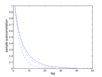
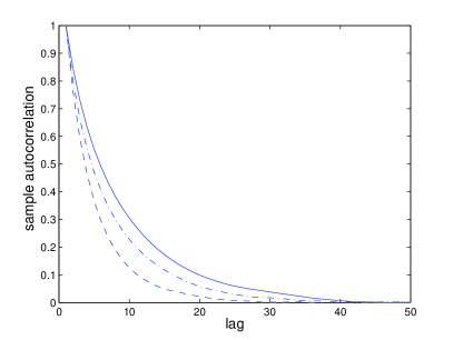
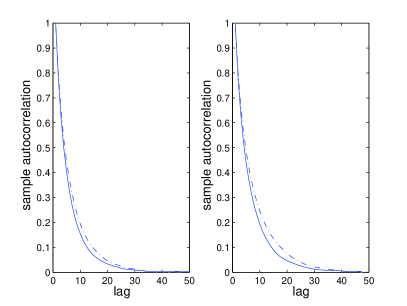
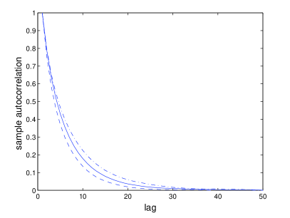
Figure 2 isolates the effect of an improper prior in PX-DA (i.e. $a=b=0$, $\kappa=\infty$). This study is restricted to PX-DA that scales the augmented data only since the prior for the value function in (16) also depends on the parameter $\kappa$ that controls the variance of the law of the translation parameter (17). Figure 2 shows the computed autocorrelation for components 4 and 7 of the estimated value function. For the proper prior, $a=5$, $b=0.5$. In this case the improper prior for the scaling parameter yields a modest improvement in performance over the proper prior. (Note though there no longer the issue of tuning the prior for the scaling parameter.)

Figure 2. PX-DA post-burn in autocorrelation plots of posterior samples for component 4 (left) and 7 (right) of the value function. Dash-dot line is PX-DA with scale move only and a proper prior with $a=5$, $b=0.5$. Solid line is PX-DA with scale move only and an improper prior.

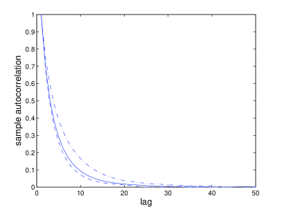
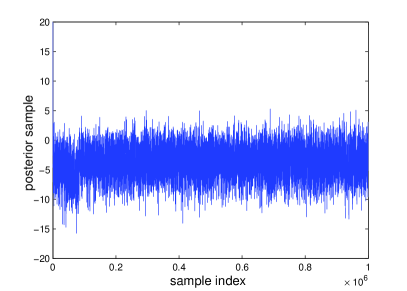
The final experiment demonstrates a situation where PX-DA converges but DA does not. The data comprising of $20$ state-action pairs of the previous examples is extended to $50$ by appending $30$ more. In this example, the priors for $V$, $Z_{1}$ and $Z_{2}$ are improper. The posterior mean of the value function calculated with PX-DA with scaling and translation is $[2.34,-0.92,-1.02,4.12,5.69,-1.79,-8.41]^{\text{T}}$. ($1.5\times 10^{6}$ posterior samples but half discarded for burn in. The posterior mean for PX-DA with scaling or translation only was practically the same.) The PX-DA implementations were initialized with the value function set to $100\times\mathbf{1}_{7}$. Shown in Figure 3 is the trace plot of the samples of component 7 of the value function obtained using the DA method initialized with the value function set to $10\times\mathbf{1}_{7}$. The mean of the second half of the samples in Figure 3 is $-3.56$. (In fact all other components of the mean of the posterior value function calculated with DA are quite far out.) In this case we see that DA fails to converge even though initialized far closer to the true values than PX-DA. Finally, to isolate the improvements due to scaling and translation, the autocorrelation plots of certain components of the posterior samples of the value function are compared in Figure 3 for PX-DA implemented with both additive and scaling, scaling only and additive only. In this example, the translation move appears more beneficial than scaling.

Figure 3. From left to right: PX-DA post-burn in autocorrelation plots of posterior samples for component 4 and 7 of the value function; and DA trace plot of posterior samples of component 7 of the value function, lack of stationarity is apparent. For the autocorrelation plots, solid line is PX-DA with translation move only, dash-dot is PX-DA with scale move only, dashed line is PX-DA with scale and translation move. The mean of the second half of the samples from DA is $-3.56$ whereas the true posterior mean (calculated with PX-DA for which the three implementations are in agreement) is $-8.4.$. It appears the DA algorithm has not converged.

5.2. Application to Human Controller Learning

In this section we apply the proposed method to an MDP which arises in the context of the popular computer game Tetris. In this game the player controls the positions and orientations of random two-dimensional shapes, henceforth the blocks, which arrive over time and occupy a field of play, henceforth the board, in a non-overlapping manner.

Figure 4. The seven blocks of Tetris.

Figure 5. Example iteration of Tetris. From left to right: 1) A block appears at the top of the board. 2) An action is taken to rotate and translate the block. 3) The block then falls until it reaches occupied squares. 4) Fully occupied rows of the board are removed.

5.2.1. Model Definition

In the MDP formulation of Tetris, the state $X=(\zeta,\eta)$ consists of two components. The first component, $\zeta$, is the current configuration of the board and is expressed as a $30\times 10$ binary matrix. The second component, $\eta$, is the index of a block. We consider $7$ distinct blocks, shown in Figure 4, and thus $\eta$ takes values in $\{1,2,...,7\}$. Each action $A$ consists of the angle through which to rotate the current block ($0^{\circ}$, $90^{\circ}$, $180^{\circ}$, $270^{\circ}$), and the number of squares by which to move it left or right. For each state not all combinations of horizontal translation and rotation are necessarily permitted as the block must remain entirely within the boundaries of the board and must not overlap with any occupied squares. We write $\mathcal{A}(x)$ for the set of actions which are valid in state $X=x$.

From the current state $X_{t}=(\zeta_{t},\eta_{t})$ and an action $A_{t}\in\mathcal{A}(X_{t})$, the evolution of the state occurs according to

(21) $$\zeta_{t+1}=\psi(\zeta_{t},\eta_{t},A_{t}), \eta_{t+1}\sim\mathcal{U}(1,2,...,7),$$

where $\psi$ is a deterministic mapping which describes the evolution of the board configuration once the action has been chosen. For a configuration $\zeta_{t}$ with no occupied squares in the top row, $\psi$ yields the new configuration $\zeta_{t+1}$ by moving the block $\eta_{t}$ according to $A_{t}$, then allowing the block to “fall” until it reaches an occupied square or the bottom row of the board, and then removing any fully occupied rows. For a configuration $\zeta_{t}$ which has an occupied square in the top row, $\psi$ sets $\zeta_{t+1}=\zeta_{t}$ irrespective of $A_{t}$ and $\eta_{t}$. The latter corresponds to “termination” of the game; once such a state is reached, subsequent actions do not influence the state. A pictorial representation of one iteration of the game is given in Figure 5.

As each state consists of a single board configuration and block type, the total number of states in the Tetris model is rather large. We therefore adopt the approach outlined in Section 4 and regress the value function on to a collection of $K$ basis functions $\{\phi_{1},\phi_{2},...,\phi_{K}\}$, which depend on the board configuration $\zeta$ but not on the randomly falling piece $\eta$. (Note that the latter is not controlled as new blocks arrive independently of the action and the previous state.) Specific details of the basis functions are given in section 5.2.

We assume that the reward is independent of the action and the action generation model is then

(22) $$A_{t}=\arg\max_{a\in\mathcal{A}(x_{t})}\left\{\epsilon_{t}(a)+\sum_{i=1}^{K}V(i)\cdot\left(\phi_{i}\circ\psi\right)(\zeta_{t},\eta_{t},a)\right\}.$$

We assume that the noise corrupting the action choice has identity covariance. The likelihood of observed data is

$$p(d|v,\Sigma)=\prod_{t=1}^{T}p(a_{t}|v,x_{t},\Sigma),$$

where for each $k=1,...,T$,

$$p(A_{t}=i\left|v,x_{t},\Sigma\right.)=\int_{\{\epsilon\in\mathbb{R}^{M_{t}}:\,\epsilon(i)\geq\epsilon(j)\mbox{ for all }j\neq i\}}\mathcal{N}(\epsilon;R_{t}v,I_{M_{t}})d\epsilon.$$

Here $M_{t}:=|\mathcal{A}(x_{t})|$ and $R_{t}$ is the $M_{t}\times N$ matrix with entries specified by

$$[R_{t}]_{ij}:=(\phi_{j}\circ\psi)(\zeta_{t},\eta_{t},i).$$

In this case the likelihood is invariant to scaling in the sense that

$$p(d|v,\sigma^{2}I)=p(d|\sqrt{z_{1}}v,z_{1}\sigma^{2}I),\;\;\;\forall z_{1}\in\mathbb{R}_{+}.$$

The sampling algorithm for inference is Algorithm 4.1.1 where the augmented data and transformation are given by

$$Y=(W_{1},\ldots,W_{T}), Y^{\prime}=\varphi_{z_{1}}^{-1}(Y)=\left(\sqrt{z_{1}}W_{1}^{\text{T}},\ldots,\sqrt{z_{1}}W_{T}^{\text{T}}\right)^{\text{T}},$$

where the scaling factor $Z_{1}\sim IG(a,b)$. The Jacobian for this transformation is

$$J_{z_{1}}(y^{\prime})=z_{1}^{-\frac{\sum_{t=1}^{T}M_{t}}{2}}.$$

The prior for $V$ is $\mathcal{N}(\mathbf{0}_{N},\kappa I_{N})$.

We consider the following $K=3$ basis functions which were found to capture various features of the board configuration. $\phi_{1}$, the height of the top-most occupied square in the board, across all the columns; $\phi_{2}$, the number of unoccupied squares which have at least one occupied square above them in the same column; $\phi_{3}$ the sum of the squared differences between occupied heights of adjacent columns.

In Tsitsiklis and Roy, (1994), Bertsekas and Tsitsiklis, (1996), for a board with $c$ columns, $\phi_{1}$, $\phi_{2}$ and $2c-1$ additional features were used to construct an automated self-improving Tetris playing system using Reinforcement Learning techniques. In contrast, the emphasis here is to make predictions about actions and mimic play on the basis of observed state-action data. In our setup the latter amounts to posterior prediction, which can be performed in the following manner. Let $\{V_{n}\}_{n=1}^{L}$ be a collection of post-burn-in samples from the posterior distribution over the value function, obtained from the PX-DA algorithm. Then for each state in a given sequence $\{(\zeta_{t},\eta_{t})\}_{t=1}^{T}$ we would like to make predictions under our model about the corresponding action, on the basis of the posterior samples $\{V_{n}\}_{n=1}^{L}$. To this end, for each $(\zeta_{t},\eta_{t})$ we define the MAP predicted action as

$$\widehat{A}_{t}^{\text{MAP}}(\zeta_{t},\eta_{t}) :=\arg\max_{a\in\mathcal{A}(x_{t})}\sum_{n=1}^{L}\mathbb{I}\left[\widehat{A}_{n,k}(\zeta_{t},\eta_{t})=a\right],$$

(23) $$\widehat{A}_{n,k}(\zeta_{t},\eta_{t}) :=\arg\max_{a\in\mathcal{A}(x_{t})}\left\{\epsilon_{n,k}(a)+\sum_{j=1}^{N}V_{n}(j)\cdot\left(\phi_{j}\circ\psi\right)(\zeta_{t},\eta_{t},a)\right\},$$

where for each $1\leq n\leq L$, $1\leq k\leq T$ and $a\in\mathcal{A}(x_{t})$, $\epsilon_{n,k}(a)$ is an independent $\mathcal{N}(0,1)$ random variable.

In the following section the predictive performance of the model is assessed for a number of data sets. Each data set is divided into two subsets. The PX-DA algorithm is used to draw samples from the posterior corresponding to the first subset and then the accuracy of the posterior prediction is assessed using the second subset. This assessment is performed in terms of the empirical action error, defined as

(24) $$\mathcal{E}_{a}:=\frac{1}{T}\sum_{t=1}^{T}\mathbb{I}\left[\widehat{A}_{t}^{\text{MAP}}(\zeta_{t},\eta_{t})\neq a_{t}\right].$$

where $\{(\zeta_{t},\eta_{t},a_{t})\}_{t=1}^{T}$ is the second data subset.

Finally we note that in practical situations computation of (23) may be expensive if $L$ is large, in which case one may resort to heuristic action prediction based on a posterior point estimate of $V$. We do not explore this issue further.

5.2.2. Experiment 1

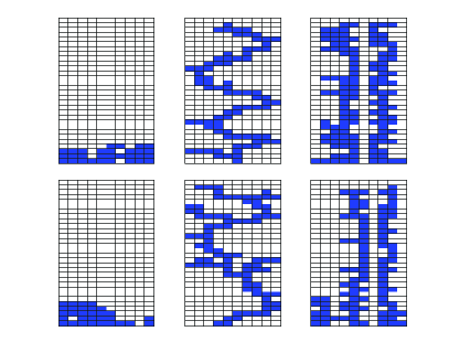
The aim of the first numerical experiment is to verify that it is possible to recover a value function and perform accurate prediction from data when the truth is known. We consider three different value functions $(-3,-15,-1)$, $(0,5,0)$ and $(-20,0,1)$. These value functions were chosen for purposes of exposition; the corresponding optimal policies lead to qualitatively distinct styles of play. Snap-shots of typical board configurations under play according to the action generation model for each of these value functions are given in the top row of Figure 7. The first value function, $(-3,-15,-1)$, led to an “efficient” style of play in which the upper region of the board is rarely occupied. The second value function, $(0,5,0)$, yields a policy which encloses many unoccupied spaces, leading to the distinctive zig–zag pattern displayed in the second columns of Figure 7. The third value function, $(-20,0,1)$, corresponds to a policy which tends to produce “towers” of occupied squares.

For each of the three value functions, $500$ observations (state/action pairs) were generated according to the model (22) with the state updated according to (21). During generation of the data, if the game terminated it was immediately restarted. For the value function $(-3,-15,-1)$, termination did not occur within $500$ time steps of the game. For the other two, termination typically occurred after $10$ to $20$ time steps so the full data record of length $500$ consisted of the concatenation of several data sets. In all three cases, the first $100$ observations were reserved for inference and the remaining $400$ used for assessment of predictive performance.

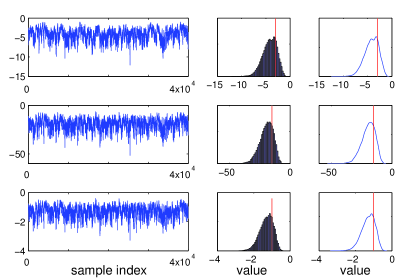
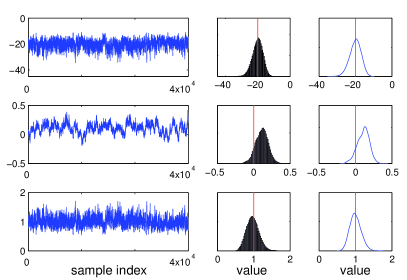
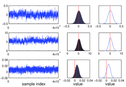
For each value function the PX-DA algorithm, incorporating the Metropolis-Hastings kernel, was run independently targeting the posterior distributions corresponding to the first $10$, $20$, $50$ and $100$ observations. In each case the algorithm was run for $5\times 10^{5}$ iterations, with a burn in of $10^{4}$ iterations. The Metropolis-Hastings acceptance rate was found to be between $0.5$ and $0.9$ in all cases. The parameters of the model were set to $\kappa=2500$ to give a relatively uninformative prior over the value function, and for the prior on the parameter $z_{1}$, $a=3$ and $b=10^{5}$. For these tuned values of $a$ and $b$, using an improper prior over $z_{1}$ led to negligible improvements in performance. Post-burn in trace plots, histograms and kernel density estimates are shown in Figure 6 along with the true value function values for the case of inference from $50$ observations. In all cases, the posterior marginals have significant mass in the neighborhood of the true value function values.

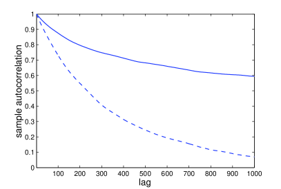
Figure 6 also shows the autocorrelation for one component of one of the value function, from the output of the PX-DA and standard DA algorithms. This indicates that the PX-DA algorithm yields a significantly lower autocorrelation than the standard DA scheme.

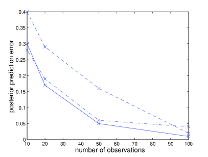
Figure 7 shows the predictive performance in terms of the prediction error $\mathcal{E}_{a}$ defined in equation (24) as a function of the number of observations used for inference. In all cases $\mathcal{E}_{a}$ was computed using the remaining $400$ observations, i.e. in (24) $T=400$. These results verify that the predictive performance improves as the number of observations used for inference increases.

The qualitative characteristics of play according to the three true value functions and according to the posterior predictions are also summarized in Figure 7. In this Figure, the top row shows snap-shots of board configurations. The bottom row shows snap-shots of play according to posterior predicted actions (with inference based on $50$ observations) for a different block sequence $\{\eta_{k}\}$ and with the state updated according to

$$\zeta_{t+1}=\psi\left(\zeta_{t},\eta_{t},\widehat{A}_{t}^{\text{MAP}}(\zeta_{k},\eta_{k})\right), \eta_{t+1}\sim\mathcal{U}(1,2,...,7).$$

These results indicate that the predicted actions result in a style of play which is qualitatively similar to that obtained from actions generated according to the true value function.

Lastly, with moves played according to $\hat{A}_{t}^{\text{MAP}}$ based on inference from the $100$ observations generated using the value function $(-3,-15,-1)$, termination of the game did not occur within $250$ time steps in $80$ out of $100$ trials. In this sense, play according to $\hat{A}_{t}^{\text{MAP}}$ compared quite well with play according to $A_{t}$, where no termination occurred within $500$ time steps.

Figure 6. Experiment 1. PX-DA post burn-in trace plots of $4\times 10^{5}$ samples, histograms and kernel density estimates of the posterior marginal distributions corresponding to $50$ observations for the three value functions. Top left: value function $(-3,-15,-1)$. Top right: $(-20,0,1)$. Bottom left: $(0,5,0)$. True values are shown with vertical lines. Bottom right: auto-correlation as a function of lag of the first component of $V$ for PX-DA (dashed) and DA (solid) algorithms in the case of the true value function $(-3,-15,-1)^{T}$, from $4\times 10^{5}$ post burn-in samples.

Figure 7. Experiment $1$. Right top row: Board snap-shots. From left to right the true value functions are $(-3,-15,-1)$, $(0,5,0)$ and $(-20,0,1)$. Right bottom row: Board snapshots during play according to posterior predictive actions for a different block sequence. Left: Posterior prediction errors as a function of the number of observations used for inference for the three value functions: $(-3,-15,-1)$ solid, $(0,5,0)$ dashed and $(-20,0,1)$ dash-dot.

5.2.3. Experiment 2

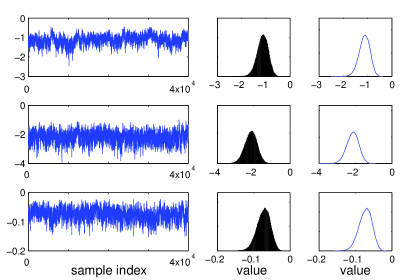
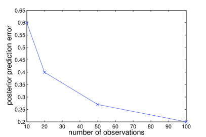
The aim of the second experiment is to demonstrate inference and prediction from a data set of a human player, i.e. in this case the true value function is unknown. The game was played for $500$ iterations and again, the first $100$ observations were reserved for inference and the subsequent $400$ observations were reserved for assessment of predictive performance. The PX-DA algorithm was run using the same settings as in Experiment 1. Again, the Metropolis-Hastings acceptance rate was found to be between $0.5$ and $0.9$. Trace plots, histograms and kernel density estimates are displayed in Figure 8 for the case of inference from $50$ observations. Figure 8 also shows the empirical action error as function of the number of observations used for inference. The result indicates that even with three basis functions, it is possible to capture significant information about the player’s policy.

Figure 8. Left: trace plots, histograms and kernel density estimates for of posterior marginals for the three components of the value function. Inference based on $50$ observations. Right: Posterior prediction error as a functions of the number of observations used for inference.

5.2.4. Experiment 3

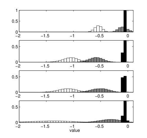
In the third experiment, the play of a human was recorded under time-pressure: at each iteration of the game a fixed time was allocated for an action to be chosen. The aim of this experiment was to validate the statistical treatment of the problem, by exhibiting the influence of the amount of data recorded on inferences drawn about a player’s action preferences. The experiment concerns a situation in which the amount of data recorded is driven by the speed at which the player is forced to play; upon the appearance of a block at the top of the board, the player was allowed $\tau$ seconds to decide how to move the block. If this time limit was exceeded, no action was recorded and the board was updated by allowing the block to fall without any rotation or translation.

Figure 9 shows histograms of post-burn-in MCMC samples approximating posterior marginals. Each panel corresponds to a different value of the time-pressure parameter $\tau$ (see caption for details). For each of the four values of $\tau$, the player was presented with the same sequence of $100$ blocks. The hyper-parameters were set to the same values as in Experiment 2. The results indicate that, as the time allocated for decision making was increased, the data provide more information about their action preferences, and this is manifested in the concentration of the posterior marginals. A striking feature is the difference between the top two panels, especially in terms of mode locations. These two panels correspond respectively to $\tau=10$ and $\tau=5$ seconds for decision making. The player made $28$ more decisions within the allocated time in the former case than in the latter, evidently leading to differences in posterior distributions over components of the value function.

Figure 9. Experiment 3. Histogram approximations of posterior marginals from MCMC output of $250\times 10^{3}$ samples. Each panel corresponds to a different constraint on the time $\tau$ allowed per decision. Top to bottom: $\tau=10,5,3,1$ seconds. The player was presented with $100$ blocks in total and made respectively/Users/sumeetpalsingh/Desktop/untitled folder/refs.bib $100,72,55,17$ decisions within the time constraints. White, grey and black shaded histograms correspond to the three components of the value function.

6. Conclusion

Our approach to inferential computation, based on an MCMC scheme, is well suited to the situation in which one is presented with a batch of state/action data. In some situations, it may be that data actually arrive gradually over time, in which case one is faced with the computational task of approximating a sequence of posterior distributions, defined as the data become available. Sequential Monte Carlo methods (Chopin,, 2002; Del Moral et al.,, 2006) are amenable to this kind of sequential inference computations and a possible extension of the work presented here is to develop such methods for the class of models we consider. Recently, Zhang and Singh, (2012) have applied the same probabilistic model and PX-DA sampler developed in this paper to Microsoft’s skill-based ranking model. The goal is to estimate the joint probability distribution of the skills of all players (where the skill of each player is represented by a real number) from the observation of the outcomes of multiple games involving subsets of these players. Preliminary results indicate that the PX-DA sampler is more accurate in predicting the outcome of games involving closely ranked players compared to Microsoft’s variational Bayes approach (called TrueSkill.) This research is being developed further by the authors.

7. Appendix

7.1. Proof of Proposition 1

The proof is essentially that of Hobert and Marchev, (2008, Proposition 3) specialized to our specific choice for the PX-DA move which comprises of both a scale and translation.

An operation on $\mathbb{R}_{+}\times\mathbb{R}$ is defined as follows. For any constants $\tilde{z}=(\tilde{z}_{1},\tilde{z}_{2}),z=(z_{1},z_{2})\in\mathbb{R}_{+}\times\mathbb{R}$, let

$$\tilde{z}z:=(\tilde{z}_{1}z_{1},\tilde{z}_{2}+\frac{z_{2}}{\tilde{z}_{1}}), z^{-1}:=(z_{1}^{-1},-z_{1}z_{2}).$$

As a consequence of these definitions, $\varphi_{\tilde{z}}(\varphi_{z}(y))=\varphi_{\tilde{z}z}(y)$, $\varphi_{z^{-1}}(\varphi_{z}(y))=\varphi_{z}(\varphi_{z^{-1}}(y))=y$ and $\varphi_{z}^{-1}(y)=\varphi_{z^{-1}}(y)$. The following equivalences may be established by routine integration. For any $z\in\mathbb{R}_{+}\times\mathbb{R}$ and integrable functions $h_{1},h_{2}:\mathbb{R}^{q}\rightarrow\mathbb{R}$, $g:\mathbb{R}_{+}\times\mathbb{R}\rightarrow\mathbb{R}$,

(25) $$\int h_{1}(\varphi_{z}(y))J_{z}(y)dy=\int h_{1}(y)dy,$$

(26) $$\int_{\mathbb{R}_{+}\times\mathbb{R}}g(z\tilde{z})dz_{1}dz_{2}=\frac{1}{\tilde{z}_{1}}\int_{\mathbb{R}_{+}\times\mathbb{R}}g(z)dz_{1}dz_{2},$$

(27) $$c(\varphi_{z}(y))=\frac{c(y)}{z_{1}J_{z}(y)},$$

(28) $$\int_{\mathbb{R}_{+}\times\mathbb{R}}g(z_{1}^{-1},-z_{1}z_{2})\frac{1}{z_{1}}dz_{1}dz_{2}=\int_{\mathbb{R}_{+}\times\mathbb{R}}g(z_{1},z_{2})dz_{1}dz_{2}.$$

(25) and (26) follow from the change of variable formula while (27) follows from (26) and the fact that

$$J_{z}(\varphi_{\tilde{z}}(y))=\frac{J_{z\tilde{z}}(y)}{J_{\tilde{z}}(y)}.$$

Then,

$$\int_{\mathbb{R}_{+}\times\mathbb{R}}\left[\int_{\mathbb{R}^{q}}h_{1}(y)h_{2}(\varphi_{z}(y))\frac{f_{Y}(\varphi_{z}(y))J_{z}(y)}{c(y)}f_{Y}(y)dy\right]dz_{1}dz_{2}$$

$$=\int_{\mathbb{R}_{+}\times\mathbb{R}}\left[\int_{\mathbb{R}^{q}}h_{1}(\varphi_{z^{-1}}(\varphi_{z}(y)))h_{2}(\varphi_{z}(y))\frac{f_{Y}(\varphi_{z}(y))J_{z}(y)}{c(\varphi_{z^{-1}}(\varphi_{z}(y)))}f_{Y}(\varphi_{z^{-1}}(\varphi_{z}(y)))dy\right]dz_{1}dz_{2}$$

$$=\int_{\mathbb{R}_{+}\times\mathbb{R}}\left[\int_{\mathbb{R}^{q}}h_{1}(\varphi_{z^{-1}}(y))h_{2}(y)\frac{f_{Y}(y)}{c(\varphi_{z^{-1}}(y))}f_{Y}(\varphi_{z^{-1}}(y))dy\right]dz_{1}dz_{2}$$

$$=\int_{\mathbb{R}^{q}}\left[\int_{\mathbb{R}_{+}\times\mathbb{R}}h_{1}(\varphi_{z^{-1}}(y))h_{2}(y)\frac{f_{Y}(y)J_{z^{-1}}(y)}{z_{1}c(y)}f_{Y}(\varphi_{z^{-1}}(y))dz_{1}dz_{2}\right]dy$$

$$=\int_{\mathbb{R}^{q}}\left[\int_{\mathbb{R}_{+}\times\mathbb{R}}h_{1}(\varphi_{z}(y))h_{2}(y)\frac{f_{Y}(y)J_{z}(y)}{c(y)}f_{Y}(\varphi_{z}(y))dz_{1}dz_{2}\right]dy$$

where the final three lines are established by invoking (25), (27) and (28). This establishes the stated reversibility.

7.2. Metropolis Hastings Kernel

For each $i=1,...,T$, one must sample $W_{i}$ from the truncated Gaussian given in (19). The procedure for performing this step is discussed below for $W_{1}$, with the subscript omitted from the notation.

Let $W(i)\sim\mathcal{N}(\mu(i),1)$ independently, $i=1,\ldots,M$. The aim is to sample the scalar random variables $W(i)$’s conditional on the event $W(i)<W(l)$, for a fixed $l$ and all $i\neq l$. Without loss of generality, take $l=1$. The corresponding distribution for the $W(i)$’s may be decomposed as follows. The marginal density of $W(1)$ is

$$p(w(1))\propto p_{u}(w(1))=\mathcal{N}(w(1);\mu(1),1)\prod_{i=2}^{M}\Phi(w(1)-\mu(i)),$$

and, conditional on $W(1)=w(1)$, $W(i)|\{W(1)=w(1)\}\sim\mathcal{TN}_{(-\infty,w(1)]}(\mu(i),1)$ for $i=2,\ldots,M$, independently, where $\Phi$ denotes the cumulative distribution function of  $\mathcal{N}(0,1)$, and $\mathcal{TN}_{[a,b]}(m,s^{2})$ stands for the $\mathcal{N}(m,s^{2})$ distribution truncated to the interval $[a,b]$.

Several efficient algorithms exists for sampling from a truncated Gaussian distribution, see Chopin, (2011). We focus on the marginal of $W(1)$. We derive an efficient independent Metropolis-Hastings step for $W(1)$ based on a $\mathcal{N}(m,s^{2})$ proposal distribution. The acceptance rate reads:

$$1\wedge\frac{p_{u}(w^{\prime}(1))\mathcal{N}(w(1);m,s^{2})}{p_{u}(w(1))\mathcal{N}(w^{\prime}(1);m,s^{2})}$$

where $w(1)$ and $w^{\prime}(1)$ denote, respectively, the current value and the proposed value $W^{\prime}(1)\sim\mathcal{N}(m,s^{2})$. The main issue is to derive a method for calculating a good Gaussian approximation $\mathcal{N}(m,s^{2})$ of $p(w(1))$.

The Gaussian approximation $\mathcal{N}(m,s^{2})$ is obtained iteratively. At each iteration, we use the following crude approximation: the function $\Phi(x)$ is replaced by constant one for $x>0$, and by function $\mathcal{N}(x;0,1)$ for $x<0$. The latter approximation is justified by the fact that, for $x\rightarrow-\infty$, $x\Phi(x)/\mathcal{N}(x;0,1)\rightarrow-1$ quickly.

At first iteration, set $(m,s^{2})=(mu(1),1)$. Then repeat the following steps: select the factor $i$ with largest $\mu(i)$ and multiply the current Gaussian approximation $\mathcal{N}(x;m_{0},s_{0}^{2})$ by either the density $\mathcal{N}(x;\mu(i),1)$ if $\mu(i)>m_{0}$, or by $1$ otherwise. Discard factor $i$ and repeat this procedure until all $M-1$ factors have been accounted for. Set $(m,s^{2})$ to be the mean and variance of this resulting proposal.

To refine this proposal, perform several Newton-Raphson iterations for finding the mode and the curvature of the mode of $\log p(w(1))$ by using $(m,s^{2})$ as the starting values. All these operations take very little time, and leads to an acceptance rate close to one in most cases. This program is available upon request.

7.3. Implementing Step 2 of Algorithm 4.1.1

The density (20) can be written as

$$\mathcal{N}\left(v;\mathbf{0}_{N-1},\kappa I_{N-1}-\kappa N^{-1}\mathbf{1}_{N-1}\mathbf{1}_{N-1}^{\text{T}}\right)\prod\limits_{i=1}^{T}\mathcal{N}(w_{i}^{\prime}-R_{i}\sqrt{z_{1}}\left(v+z_{2}\mathbf{1}_{N}\right);\mathbf{0}_{M},z_{1}I_{M})$$

(29) $$\times\mathcal{N}(z_{2};0,\kappa N^{-1})IG(z_{1};a,b).$$

By implementing the change of variable

$$(v(1),\ldots,v(N-1),z_{2})$$

(30) $$\rightarrow(u(1),\ldots,u(N))=\sqrt{z_{1}}\left(\left[v(1),\ldots,v(N-1),-\sum_{i=1}^{N-1}v(i)\right]+z_{2}\mathbf{1}_{N}^{\text{T}}\right),$$

(29) becomes

$$\mathcal{N}\left(u;\mathbf{0}_{N},\kappa z_{1}I_{N}\right)\prod\limits_{i=1}^{T}\mathcal{N}(w_{i}^{\prime}-R_{i}u;\mathbf{0}_{M},z_{1}I_{M})\times IG(z_{1};a,b).$$

Sampling $(U,Z_{1})$ is now straightforward:

$$Z_{1}\sim IG(\frac{TM}{2}+a,b+SSR/2+H/2),\quad U|Z_{1}=z_{1}\sim\mathcal{N}(\frac{1}{z_{1}}S^{-1}\widetilde{R}^{\text{T}}\widetilde{w},S^{-1}).$$

where

$$SSR=\widetilde{w}^{\text{T}}\widetilde{w}-\widetilde{w}^{\text{T}}\widetilde{R}(\widetilde{R}^{\text{T}}\widetilde{R})^{-1}\widetilde{R}^{\text{T}}\widetilde{w}, u_{LS}=(\widetilde{R}^{\text{T}}\widetilde{R})^{-1}\widetilde{R}^{\text{T}}\widetilde{w},$$

$$H=u_{LS}^{\text{T}}(I_{N}\kappa+(\widetilde{R}^{\text{T}}\widetilde{R})^{-1})^{-1}u_{LS}, S=I_{N}z_{1}^{-1}\kappa^{-1}+z_{1}^{-1}(\widetilde{R}^{\text{T}}\widetilde{R}).$$

and $\widetilde{w}^{\text{T}}=\left[(w_{1}^{\prime})^{\text{T}},\ldots,(w_{T}^{\prime})^{\text{T}}\right]$, $\widetilde{R}^{\text{T}}=\left[R_{1}^{\text{T}},\ldots,R_{T}^{\text{T}}\right]$. Here $u_{LS}$ refers to the least squares estimate of $u$ and $SSR$ is the minimum mean-squared error. To recover $(V,Z_{2})$ from $(U,Z_{1})$, let $u$ denote the sampled random vector $U$, then $(Z_{2},V)$ is obtained as $\left(z_{1}^{-1/2}\frac{\boldsymbol{1}_{N}^{\text{T}}u}{N},z_{1}^{-1/2}(u-\frac{\boldsymbol{1}_{N}^{\text{T}}u}{N}\boldsymbol{1}_{N})\right)$.

References

- Abbeel and Ng, (2004) Abbeel, P. and Ng, A. (2004). Apprenticeship learning via inverse reinforcement learning. In Brodley, C., editor, Proceedings of the Twenty-first International Conference on Machine Learning, volume 69, Banff, Alberta, Canada. ACM.
- Aguirregabiria and Mira, (2002) Aguirregabiria, V. and Mira, P. (2002). Swapping the nested fixed point algorithm: a class of estimators for discrete Markov decision models. Econometrica, 70:1519 –1543.
- Albert and Chib, (1993) Albert, J. and Chib, S. (1993). Bayesian analysis of binary and polychotomous response data. Journal of the American Statistical Association, 88(422):669–679.
- Bertsekas, (2005) Bertsekas, D. (2005). Dynamic programming and optimal control. Vol. 1, 3rd Ed. Athena Scientific, Belmont, Mass.
- Bertsekas, (2007) Bertsekas, D. (2007). Dynamic programming and optimal control. Vol. 2, 3rd Ed. Athena Scientific, Belmont, Mass.
- Bertsekas and Tsitsiklis, (1996) Bertsekas, D. and Tsitsiklis, J., editors (1996). Neuro-dynamic programming. Athena Scientific, Belmont.
- Chopin, (2002) Chopin, N. (2002). A sequential particle filter method for static models. Biometrika, 89(3):539–552.
- Chopin, (2011) Chopin, N. (2011). Fast simulation of truncated gaussian distributions. Statistics and Computing, 21(2):275–288.
- Coates et al., (2009) Coates, A., Abbeel, P., and Ng, A. Y. (2009). Apprenticeship learning for helicopter control. Commun. ACM, 52:97–105.
- Del Moral et al., (2006) Del Moral, P., Doucet, A., and Jasra, A. (2006). Sequential Monte Carlo samplers. Journal of the Royal Statistical Society: Series B (Statistical Methodology), 68(3):411–436.
- Geweke and Keane, (1996) Geweke, J. and Keane, M. (1996). Bayesian inference for dynamic discrete choice models without the need for dynamic programming. Working Paper 564, Federal Reserve Bank of Minneapolis.
- Geweke and Keane, (2000) Geweke, J. and Keane, M. (2000). Bayesian inference for dynamic discrete choice models without the need for dynamic programming. In Mariano, R., Schuermann, T., and Weeks, M., editors, Simulation-based inference in econometrics: methods and applications, chapter 4, pages 100–131. Cambridge University Press, Cambridge.
- Geweke et al., (1994) Geweke, J., Keane, M., and Runkle, D. (1994). Alternative computational approaches to inference in the multinomial probit model. Review of Economics and Statistics, pages 609–632.
- Gotz and McCall, (1980) Gotz, G. and McCall, J. (1980). Estimation in sequential decision making models: a methodological note. Economic Letters, 6:131 –136.
- Hobert, (2011) Hobert, J. (2011). The data augmentation algorithm: theory and methodology. In Handbook of Markov Chain Monte Carlo, pages 253–293. Chapman & Hall/CRC Handbooks of Modern Statistical Methods.
- Hobert and Marchev, (2008) Hobert, J. and Marchev, D. (2008). A theoretical comparison of data augmentation, marginal augmentation and PX-DA algorithms. The Annals of Statistics, 36(2):532 –554.
- Hotz and Miller, (1993) Hotz, J. and Miller, R. (1993). Conditional choice probabilities and estimation of dynamic models. Review of Economic Studies, 60:497–529.
- Imai and van Dyk, (2005) Imai, K. and van Dyk, D. (2005). A Bayesian analysis of the multinomial probit model using marginal data augmentation. Journal of Econometrics, 124:311–334.
- Imai et al., (2009) Imai, S., Jain, N., and Ching, A. (2009). Bayesian estimation of dynamic discrete choice models. Econometrica, 77(6):1865–1899.
- Liu and Wu, (1999) Liu, J. and Wu, Y. (1999). Parameter expansion for data augmentation. Journal of the American Statistical Association, 94:1264 –1274.
- McCulloch et al., (2000) McCulloch, R., Polson, N., and Rossi, P. (2000). A Bayesian analysis of the multinomial probit model with fully identified parameters. Journal of Econometrics, 99:172–193.
- McCulloch and Rossi, (1994) McCulloch, R. and Rossi, P. (1994). An exact likelihood analysis of the multinomial probit model. Journal of Econometrics, 64:207–240.
- Meng and van Dyk, (1999) Meng, X.-L. and van Dyk, D. (1999). Seeking efficient data augmentation schemes via conditional and marginal augmentation. Biometrika, 86:301–320.
- Ng and Russell, (2000) Ng, A. and Russell, S. (2000). Algorithms for inverse reinforcement learning. In Langley, P., editor, Proceedings of the Seventeenth International Conference on Machine Learning, pages 663–670, San Franciso, CA. Morgan Kaufmann.
- Nobile, (1998) Nobile, A. (1998). A hybrid Markov chain for Bayesian analysis of the multinomial probit model. Statistics and Computing, 8:229–242.
- Roy, (2012) Roy, V. (2012). Spectral analytic comparisons for data augmentation. Statistics and Probability Letters, 82(1):103–108.
- Rust, (1987) Rust, J. (1987). Optimal replacement of GMC bus engines: an empirical model of Harold Zurcher. Econometrica, 55:999–1033.
- Rust, (1988) Rust, J. (1988). Maximum likelihood estimation of discrete control processes. SIAM Jour. Control and Optim., 26:1006–1024.
- Schmajuk and Zanutto, (1997) Schmajuk, N. A. and Zanutto, B. S. (1997). Escape, Avoidance, and Imitation: A Neural Network Approach. Adaptive Behavior, 6(1):63–129.
- Schweitzer and Seidmann, (1985) Schweitzer, P. J. and Seidmann, A. (1985). Generalized polynomial approximations in markovian decision processes. Journal of Mathematical Analysis and Applications, 110(2):568–582.
- Tanner and Wong, (1987) Tanner, M. and Wong, W. (1987). The calculation of posterior distributions by data augmentation (with discussion). Journal of the American Statistical Association, 82:528–550.
- Tsitsiklis and Roy, (1994) Tsitsiklis, J. and Roy, B. V. (1994). Feature-based methods for large scale dynamic programming. Technical Report LIDS-P 2277, Massachusetts Institute of Technology, Laboratory for Information and Decision Systems.
- Watkins, (1987) Watkins, C. (1987). Learning from delayed rewards. PhD thesis, University of Cambridge.
- Wolpin, (1984) Wolpin, K. (1984). An estimable dynamic stochastic model of fertility and child mortality. Journal of Political Economy, 92:852 –874.
- Zhang and Singh, (2012) Zhang, X. and Singh, S. (2012). A comparison of Trueskill and Gibbs sampling. Unpublished report.