Classical heat transport in anharmonic molecular junctions: exact solutions

Abstract

We study full counting statistics for classical heat transport through anharmonic/nonlinear molecular junctions formed by interacting oscillators. Analytical result of the steady state heat flux for an overdamped anharmonic junction with arbitrary temperature bias is obtained. It is found that the thermal conductance can be expressed in terms of temperature dependent effective force constant. The role of anharmonicity is identified. We also give the general formula for the second cumulant of heat in steady state, as well as the average geometric heat flux when two system parameters are modulated adiabatically. We present an anharmonic example for which all cumulants for heat can be obtained exactly. For a bounded single oscillator model with mass we found that the cumulants are independent of the nonlinear potential.

I Introduction

Anharmonicity or nonlinearity plays an important role in many physical processes. For example, it is crucial for umklapp scattering which gives rise to a finite thermal conductivity for bulk systems as pointed out by Peierls Peierls (1955). It is also an essential ingredient required for developing functional phononic devices Li et al. (2012), such as thermal rectifier Terraneo et al. (2002); Chang et al. (2006) and heat pump Segal and Nitzan (2006); Segal (2008); Ren et al. (2010).

Comprehensive understanding of the general behaviors of nonlinearity in transport is a fundamental problem in condensed matter physics and nonequilibrium statistical physics. Although elegant approaches exist to deal with ballistic transport in harmonic systems Dhar and Roy (2006); Wang et al. (2008), solving an anharmonic model analytically is extremely challenging due to the intrinsic non-integrability of equations of motion. As a result, for classical heat transport, the major approaches are limited to molecular dynamics simulations Lepri et al. (2003); Dhar (2008), perturbation theories such as Boltzmann equation Peierls (1955); Pereverzev (2003), mode coupling theory Lepri et al. (1998); Delfini et al. (2007), and/or mean–field theory Li et al. (2006); He et al. (2008). There does not exist analytic solutions of heat transport problem for general anharmonic potentials.

Moreover, in heat transport problems, not only the heat flux, but also the higher order fluctuations (noises) are of significant interest as they contain valuable information about the transport properties and satisfy universal symmetry known as Fluctuation Theorems (FT) Jarzynski (1997); Crooks (1999); Gallavotti and Cohen (1995). Therefore, methods to obtain these higher order moments and to verify this symmetry for arbitrary anharmonic potentials are also highly desirable.

In this article, we present a general approach to nonlinear heat transport by working in an enlarged space, which includes the heat $Q$ as an extra variable in the Fokker-Planck (FP) equation Ren et al. (2012). The heat current can be expressed as the expectation value of certain operator. If the steady state of the problem is known, then the analytic expression for the current can be obtained. We show this is the case for two different anharmonic oscillator systems, i.e., the overdamped interacting double-oscillator model (Model I) and the bounded single-oscillator model (Model II).

For Model I, the complete cumulants, as well as the geometric contribution to the heat flux, can be obtained if the full spectrum of the original FP equation is solvable. One such example is the V-shaped potential $V(y)=k|y|$. For Model II, the complete cumulants can always be analytically obtained no matter what the nonlinear interacting potential is. For both models, the Gallavotti-Cohen (GC) symmetry can be verified for arbitrary anharmonic interactions.

In the rest of the article, Sec. II is devoted to Model I and Sec. III is devoted to Model II. After that, we briefly summarize the article in Sec. IV.

II Model I

Model I consists of two coupled Brownian oscillators which are connected to two Langevin heat baths (Fig. 1(a)). The dynamics is described by the Langevin equations: $m_{i}\ddot{x}_{i}=-\partial_{x_{i}}{V}(x_{1}-x_{2})-\gamma_{i}\dot{x}_{i}+\xi_{i}$, ($i=1,2$), where $m_{i}$ and $x_{i}$ are the mass and displacement of oscillator $i$. $\gamma_{i}$ is the coupling strength between the oscillator $i$ and the bath $i$, $T_{i}$ is the temperature of bath $i$ and $\xi_{i}$ is a white noise with variance $\left\langle\xi_{i}(t)\xi_{j}(t^{\prime})\right\rangle=2\gamma_{i}T_{i}\delta_{ij}\delta(t-t^{\prime})$ ($k_{B}$ is set to 1). $V$ depicts the interaction potential, which is assumed to be bounded and depend only on the distance between the two oscillators.

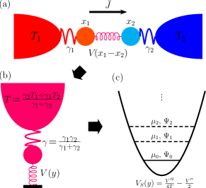
Figure 1: Schematic picture for the process of mathematical formalism for model I. (a) The original problem: two coupled oscillators connected to heat baths. (b) The reduced problem: single particle in contact with single heat bath. (c) The ultimate problem: Schrödinger equation for a single particle.

This model is a minimal model for heat transport in interacting oscillator systems. At low Reynolds number, we can neglect the inertia and thus obtain the overdamped dynamics Purcell (1977):

$$\gamma_{1}\dot{x}_{1}+V^{\prime}(x_{1}-x_{2})=\xi_{1};$$ (1)

$$\gamma_{2}\dot{x}_{2}-V^{\prime}(x_{1}-x_{2})=\xi_{2},$$ (2)

in which the prime ^′ denotes the derivative with respect to its argument. The total heat transferred from bath 1 to bath 2 up to time $t$, denoted as $Q(t)$, satisfy

$$\dot{Q}=V^{\prime}(x_{1}-x_{2})\dot{x}_{1}.$$ (3)

By introducing the relative coordinate $y=x_{1}-x_{2}$, we obtain two stochastic differential equations for the random variables $y$ and $Q$:

$$\dot{y} =-\frac{V^{\prime}(y)}{\gamma_{1}}-\frac{V^{\prime}(y)}{\gamma_{2}}+\frac{\xi_{1}}{\gamma_{1}}-\frac{\xi_{2}}{\gamma_{2}};$$ (4)

$$\dot{Q} =\frac{V^{\prime}(y)}{\gamma_{1}}\left(\xi_{1}-V^{\prime}(y)\right).$$ (5)

Their joint probability distribution $\rho(y,Q,t)$ then evolves according to the FP equation Risken (1998); Kundu et al. (2011)

$$\begin{split}\frac{\partial{\rho}}{\partial{t}}=&\left[\frac{T}{\gamma}\frac{\partial^{2}{}}{\partial{y}^{2}}+\frac{1}{\gamma}\frac{\partial{}}{\partial{y}}V^{\prime}+\frac{T_{1}}{\gamma_{1}}\frac{\partial^{2}{}}{\partial{Q}^{2}}V^{\prime 2}\right.\\ &\left.+\frac{\partial{}}{\partial{Q}}\left(\frac{V^{\prime 2}}{\gamma_{1}}-\frac{T_{1}V^{\prime\prime}}{\gamma_{1}}\right)+\frac{2T_{1}}{\gamma_{1}}\frac{\partial^{2}}{\partial Q\partial y}V^{\prime}\right]\rho,\\ \end{split}$$ (6)

where $\frac{1}{\gamma}=\frac{1}{\gamma_{1}}+\frac{1}{\gamma_{2}}$ and $\frac{T}{\gamma}=\frac{T_{1}}{\gamma_{1}}+\frac{T_{2}}{\gamma_{2}}$.

By taking the Fourier transformation on $Q$ in Eq. (6), we obtain the equation for the characteristic function (CF) $z(y,i\chi,t)=\int\rho(y,Q,t)e^{i\chi Q}dQ$, where $\int$ is short for $\int_{-\infty}^{\infty}$ throughout the paper. Moreover, we introduce $\lambda\equiv i\chi$ and use tilde ( $\tilde{}$ ) to express the $\lambda$-dependence (in such a notation, $\lambda$ is omitted in the parameter list). Then the equation reads

$$\partial_{t}{\tilde{z}(y,t)}=\tilde{L}\tilde{z}(y,t)$$ (7)

with twisted FP operator

$$\begin{split}\tilde{L}=&\frac{T}{\gamma}\frac{\partial^{2}{}}{\partial{y}^{2}}+\frac{1}{\gamma}\frac{\partial{}}{\partial{y}}V^{\prime}+\\ &\lambda\left(\frac{T_{1}V^{\prime\prime}}{\gamma_{1}}-\frac{V^{\prime 2}}{\gamma_{1}}-\frac{2T_{1}}{\gamma_{1}}\frac{\partial{}}{\partial{y}}V^{\prime}\right)+\lambda^{2}\frac{T_{1}V^{\prime 2}}{\gamma_{1}}\\ \equiv&L^{(0)}+\lambda L^{(1)}+\lambda^{2}L^{(2)},\end{split}$$ (8)

For any quantity or operator $\tilde{\mathcal{A}}$, We shall also use $\mathcal{A}$ to be short for $\tilde{\mathcal{A}}$ evaluated at $\lambda=0$. For example, $L=\tilde{L}(\lambda=0)=L^{(0)}$ and $z(y,t)=\int\rho(y,Q,t)dQ$ is the probability distribution for $y$. Moreover, for $\lambda=0$, the equation $\partial_{t}{z}(y,t)=Lz(y,t)$ actually depicts a single Brownian oscillator connected with a single heat bath at an effective temperature $T$ and subjected to a potential $V$ (see Fig. 1(b)). Therefore, the stationary solution will be in the form of Boltzmann distribution $z(y,t)\to P^{\mathrm{st}}_{T}(y)=\frac{1}{Z_{T}}e^{-V(y)/T}$ with $Z_{T}=\int e^{-V(y)/T}dy$ as the partition function.

We are only interested in the heat $Q$. Therefore, by integrating over $y$, we obtain the CF of $Q$ as $\tilde{Z}(t)=\int\tilde{z}(y,t)dy=\int P_{Q}(Q,t)e^{\lambda Q}dQ$, with $P_{Q}(Q,t)=\int\rho(y,Q,t)dy$. The cumulant generating function (CGF) reads $\tilde{G}\equiv\ln{\tilde{Z}}$, which generates the $n$th-order cumulant as $\left\langle\!\left\langle Q^{n}\right\rangle\!\right\rangle=\left.\partial_{\lambda}^{n}{\tilde{G}}\right|_{\lambda=0}$.

Obviously, if we are able to solve Eq. (7) for general potential $V$, then the problem can be completely solved, which is the case for harmonic potential Ren et al. (2012). For anharmonic cases, a general method is not available.

However, using separation of variables $\tilde{z}(y,t)=\tilde{\varphi}(y)\tilde{F}(t)$, Eq. (7) can still be casted into an eigenvalue problem

$$\tilde{F}(t)=e^{-\tilde{\mu}t},\quad\quad\tilde{L}\tilde{\varphi}(y)=-\tilde{\mu}\tilde{\varphi}(y).$$ (9)

with natural boundary conditions for $y\to\pm\infty$. The structure of the solutions is clearer if we introduce a transformation $\tilde{\varphi}(y)=e^{-{V(y)}/{2\tilde{T}}}\tilde{\Psi}(y)$ with $\tilde{T}=(\frac{T_{1}}{\gamma_{1}}+\frac{T_{2}}{\gamma_{2}})/(\frac{1}{\gamma_{1}}+\frac{1}{\gamma_{2}}-\frac{2T_{1}}{\gamma_{1}}\lambda)$. By direct substitution, it turns out that $\tilde{\Psi}(y)$ satisfy the following time independent Schrödinger equation

$$\tilde{L}_{S}\tilde{\Psi}\equiv\frac{1}{\gamma}\left(-T\frac{\partial^{2}{}}{\partial{y}^{2}}+\tilde{V}_{S}\right)\tilde{\Psi}=\tilde{\mu}\tilde{\Psi},$$ (10)

which describes a single particle moving in the effective potential $\tilde{V}_{S}$ (see Fig. 1(c)), given by

$$\tilde{V}_{S}=\frac{V^{\prime 2}}{4T}\left[1+\frac{4T_{1}T_{2}\gamma}{\gamma_{1}+\gamma_{2}}\lambda\!\left(\!\frac{1}{T_{1}}\!-\!\frac{1}{T_{2}}-\lambda\!\right)\right]-\frac{1}{2}V^{\prime\prime}.$$ (11)

Then the well-known results in quantum mechanics for single particle can be directly evoked to discuss our situation. Two of them are that all the eigenvalues are real (regard $\lambda$ as a real quantity) which can be ordered as $\quad\tilde{\mu}_{0}\leq\tilde{\mu}_{1}\leq\cdots$, and upon normalization, all the eigenfunctions form a complete orthonormal basis set, which satisfy $(\tilde{\Psi}_{n},\tilde{\Psi}_{m})=\delta_{nm}$ and $\quad\sum_{n=0}^{\infty}\tilde{\Psi}_{n}(y)\tilde{\Psi}_{n}(y^{\prime})=\delta(y-y^{\prime}).$ We use $(f,g)$ to denote the inner product $\int f(y)g(y)dy$.

The original operator $\tilde{L}$ is not Hermitian, i.e., $\tilde{L}^{\dagger}\neq\tilde{L}$. However, it can be shown that $\tilde{\phi}_{n}=e^{V/2\tilde{T}}\tilde{\Psi}_{n}$ satisfy $\tilde{L}^{\dagger}\tilde{\phi}_{n}=\tilde{\mu}_{n}\tilde{\phi}_{n}$, namely, $\tilde{\phi}_{n}$ is an eigenfunction of $\tilde{L}^{\dagger}$ with eigenvalue $\tilde{\mu}_{n}$. When normalized properly, we will have

$$(\tilde{\phi}_{n},\tilde{\varphi}_{m})=\delta_{nm},\quad\sum_{n=0}^{\infty}\tilde{\phi}_{n}(y)\tilde{\varphi}_{n}(y^{\prime})=\delta(y-y^{\prime}).$$ (12)

Then we can write down the formal solution of Eq. (7) as

$$\tilde{z}(y,t)=\sum_{n=0}^{\infty}\tilde{c}_{n}e^{-\tilde{\mu}_{n}t}\tilde{\varphi}_{n}(y),$$ (13)

where $\tilde{c}_{n}$ is time independent and can be determined using the initial condition, $\tilde{c}_{n}=\left(\tilde{\phi}_{n},\tilde{z}(y,t=0)\right)$.

II.1 Dynamic Heat Fluxes

Based on the formalism above, we come to discuss the heat fluxes in nonequilibrium steady state. It should be pointed out that the discussions here are also applicable to the dynamic heat fluxes Ren et al. (2010, 2012) when system parameters are modulated adiabatically.

If the long-time behavior is of main interest, then the component with smallest eigenvalue ($\tilde{\mu}_{0}$) will dominate, so that $\tilde{z}(y,t)\to\tilde{c}_{0}e^{-\tilde{\mu}_{0}t}\tilde{\varphi}_{0}(y)$ and $\tilde{Z}(t)\to\tilde{c}_{0}e^{-\tilde{\mu}_{0}t}\int\tilde{\varphi}_{0}(y)dy$. Consequently, the CGF $\ln{\tilde{Z}(t)}\to-\tilde{\mu}_{0}t$ and the $n$th cumulant of the heat fluctuations are given by

$$\lim_{t\to\infty}\frac{\left\langle\!\left\langle Q^{n}\right\rangle\!\right\rangle}{t}=-\left.\frac{\partial^{n}{\tilde{\mu}_{0}}}{\partial{\lambda}^{n}}\right|_{\lambda=0}.$$ (14)

Of course, one would not be able to get all the cumulants unless $\tilde{\mu}_{0}$ can be obtained as a function of $\lambda$. However, if one is only interested in the first cumulant, i.e., the average heat flux $\bar{J}=\lim_{t\to\infty}\left\langle\!\left\langle Q\right\rangle\!\right\rangle/t=-\left.\partial_{\lambda}{\tilde{\mu}_{0}}\right|_{\lambda=0}$, then here is an approach.

We differentiate Eq. (9) with respect to $\lambda$ and obtain

$$(\partial_{\lambda}{\tilde{L}})\tilde{\varphi}_{0}+\tilde{L}\partial_{\lambda}{\tilde{\varphi}_{0}}=-(\partial_{\lambda}{\tilde{\mu}_{0}})\tilde{\varphi}_{0}-\tilde{\mu}_{0}\partial_{\lambda}{\tilde{\varphi}_{0}}.$$ (15)

Then we perform $(\tilde{\phi}_{0},\cdots)$ on both sides. Noticing that $(\tilde{\phi}_{0},\tilde{L}\partial_{\lambda}{\tilde{\varphi}_{0}})=(\tilde{L}^{\dagger}\tilde{\phi}_{0},\partial_{\lambda}{\tilde{\varphi}_{0}})=-\tilde{\mu}_{0}(\tilde{\phi}_{0},\partial_{\lambda}{\tilde{\varphi}_{0}})$, we obtain

$$\bar{J}=-\left.\partial_{\lambda}{\tilde{\mu}_{0}}\right|_{\lambda=0}=\left.\left(\tilde{\phi}_{0},(\partial_{\lambda}{\tilde{L}})\tilde{\varphi}_{0}\right)\right|_{\lambda=0}=\left(\phi_{0},L^{(1)}\varphi_{0}\right).$$ (16)

This equation is the analogue of the Hellmann-Feynman theorem in quantum mechanics. Note that $\phi_{0}$ and $\varphi_{0}$ in Eq. (16) are evaluated at $\lambda=0$, therefore, are associated with the FP operator $L=L^{(0)}$. It can be shown that the smallest eigenvalue for $L(L^{\dagger})$ is $\mu_{0}=0$ and the corresponding eigenfunctions are $\varphi_{0}(y)\propto e^{-V(y)/T}\propto P^{\mathrm{st}}_{T}$ and $\phi_{0}(y)\propto 1,$ respectively Risken (1998).

After normalization, Eq. (16) becomes $\bar{J}=\int L^{(1)}P^{\mathrm{st}}_{T}(y)dy$. In this sense, $L^{(1)}$ serves as the heat flux operator, which gives the average heat flux when acted on the stationary state. Using $L^{(1)}=\frac{1}{\gamma_{1}}(T_{1}V^{\prime\prime}-V^{\prime 2}-2T_{1}\frac{\partial{}}{\partial{y}}V^{\prime})$, we finally obtain

$$\bar{J}=\frac{T_{1}}{\gamma_{1}}\left\langle V^{\prime\prime}\right\rangle_{T}-\frac{1}{\gamma_{1}}\left\langle V^{\prime 2}\right\rangle_{T}=\frac{\left\langle V^{\prime\prime}\right\rangle_{T}}{\gamma_{1}+\gamma_{2}}(T_{1}-T_{2}),$$ (17)

where $\left\langle\mathcal{A}\right\rangle_{T}\equiv\int\mathcal{A}P^{\mathrm{st}}_{T}dy$ is the canonical ensemble average of $\mathcal{A}$ at temperature $T$ and we have used $\left\langle V^{\prime 2}\right\rangle_{T}=T\left\langle V^{\prime\prime}\right\rangle_{T}$. Remember that $T=(\gamma_{2}T_{1}+\gamma_{1}T_{2})/(\gamma_{1}+\gamma_{2})$.

Equation (17) is exact for a general potential $V$. It is also applicable to the cases with arbitrarily large temperature differences, i.e., the cases in a far-from-equilibrium state. As far as we know, this is the first exact result for anharmonic heat transport with general interaction, although it is only for a small system with overdamped dynamics.

For harmonic potential $V=\frac{1}{2}ky^{2}$, $\left\langle V^{\prime\prime}\right\rangle_{T}=k$, which is just the force constant and is independent of the temperature. For anharmonic potentials, $\left\langle V^{\prime\prime}\right\rangle_{T}$ will generally be temperature dependent. In analogy with the harmonic case, we define $k_{V}(T)\equiv\left\langle V^{\prime\prime}\right\rangle_{T}$ as the effective force constant.

We notice that the temperature dependence of the effective force constant plays a key role in many of the phenomena for heat control and management. For example, a thermal rectifier is a device that directs the flow of heat Terraneo et al. (2002); Chang et al. (2006). To use this oscillator system as a thermal rectifier, it is required that

$$\left|\frac{\bar{J}(T_{1}=T_{H},T_{2}=T_{L})}{\bar{J}(T_{1}=T_{L},T_{2}=T_{H})}\right|=\frac{\left\langle V^{\prime\prime}\right\rangle_{T=\frac{\gamma_{2}T_{H}+\gamma_{1}T_{L}}{\gamma_{1}+\gamma_{2}}}}{\left\langle V^{\prime\prime}\right\rangle_{T=\frac{\gamma_{2}T_{L}+\gamma_{1}T_{H}}{\gamma_{1}+\gamma_{2}}}}\neq 1.$$ (18)

Obviously, this condition is satisfied only when $k_{V}(T)$ is temperature dependent and the system is asymmetric, namely, $\gamma_{1}\neq\gamma_{2}$.

As another example, in Li et al. (2009), it was demonstrated that heat can be shuttled across a symmetric system when the temperature of one heat bath is modulated adiabatically but with zero average temperature bias, e.g., $T_{1}=T_{2}+f(t)$ with $\overline{f(t)}=0$. If our system is modulated in such a way with $\gamma_{1}=\gamma_{2}=2\gamma$ and $f(t)$ being a periodic function of $t$, one can obtain an average heat flux $\bar{J}=\frac{1}{4\gamma T_{p}}\int_{0}^{T_{p}}k_{V}\!\!\left(\!\frac{2T_{2}+f(t)}{2}\!\right)\ f(t)dt$ in one period. Again, $\bar{J}$ is nonzero only if $k_{V}(T)$ depends on $T$. Actually, when $f(t)\ll T_{2}$, we can expand $k_{V}(\frac{2T_{2}+f(t)}{2})$ into Taylor series and obtain the leading term as $\bar{J}\approx{k^{\prime}_{V}(T_{2})}\overline{f^{2}(t)}/{8\gamma}$, where ^′ denotes derivative and $\overline{\cdots}$ denotes time average over one period. This pump effect is more significant if $k^{\prime}_{V}(T_{2})$ is larger; and is vanishing when $k^{\prime}_{V}(T_{2})=0$.

Since the effective force constant is independent of $T$ for harmonic potential, the phenomena mentioned above cannot be observed using harmonic potential. On the other hand, is harmonic potential the only potential that has such a property? The answer is no. An example is the Toda potential $V=k(e^{-ax}+ax)$ for which $\left\langle V^{\prime\prime}\right\rangle_{T}=ka^{2}$. Interestingly, both the harmonic lattice and Toda lattice are models displaying ballistic heat transport. These facts imply a clue that temperature independent $k_{V}(T)$ is related to ballistic transport.

It is worth mentioning that there are other approximated mean–field theories trying to convert an anharmonic potential in lattices to effective harmonic potential with temperature dependent force constant. For example, for the FPU-$\beta$ model with $V=\frac{k_{2}}{2}y^{2}+\frac{k_{4}}{4}y^{4}$, the effective phonon theory (EPT) estimates it as $k^{\mathrm{EPT}}(T)=k_{2}+k_{4}(\left\langle y^{4}\right\rangle_{T})/(\left\langle y^{2}\right\rangle_{T})$Li et al. (2006, 2010) while the self-consistent phonon theory (SCPT) estimates it as $k^{\mathrm{SCPT}}(T)=\frac{1}{2}\left(k_{2}+\sqrt{k_{2}^{2}+12k_{4}T}\right)$He et al. (2008). In Fig. 2, we compare these results with the present exact result for the two-oscillator model, i.e., $k^{\mathrm{exact}}(T)=k_{2}+3k_{4}\left\langle y^{2}\right\rangle_{T}$. It is shown that both the EPT and SCPT underestimate the nonlinear effect, although at low temperature the deviations are tiny. At the high temperature regime, all these theories result in the $\sim cT^{1/2}$ dependence. For $k_{2}=k_{4}=1$, the coefficient $c$ is $6\Gamma(3/4)/\Gamma(1/4)\approx 2.028$ for the exact value. For the EPT $c=\Gamma(1/4)/2\Gamma(3/4)\approx 1.479$ and for the SCPT $c=\sqrt{3}\approx 1.732$, which are 27% and 14% less than the exact value, respectively.

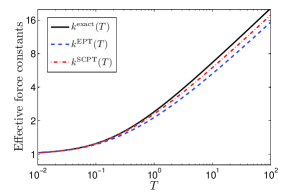
Figure 2: Effective force constant from different theories for the FPU-$\beta$ model with $k_{2}=1$ and $k_{4}=1$.

Upto now we only discussed the first cumulant, i.e., the average heat flux. However, using the standard perturbation theory, all higher order cumulants can be derived. For example, the second cumulant reads (see for example Szabo and Ostlund (1996))

$$\lim_{t\to\infty}\frac{\left\langle\!\left\langle Q^{2}\right\rangle\!\right\rangle}{t}=2L^{(2)}_{00}+2\sum_{m=1}^{\infty}\frac{L^{(1)}_{0m}L^{(1)}_{m0}}{\mu_{m}-\mu_{0}},$$ (19)

where $\mathcal{A}_{mn}\equiv\left(\phi_{m},\mathcal{A}\varphi_{n}\right)$ for short. Note that all the terms in the formula are again evaluated at $\lambda=0$.

The excited states are involved in the expression for higher order cumulants. Therefore, to analytically obtain the higher order cumulants, we should be able to completely solve all the eigenstates of the Schrödinger equation Eq. (10) with $\lambda=0$, which describes a single particle with mass $T$ moving in the potential $V_{S}=V^{\prime 2}/4T-V^{\prime\prime}/2$ (see Fig. 1(c)). This is of course an impossible mission for most of the anharmonic potentials. However, numerically solving it by diagonalizing the operator $L_{S}$ is straightforward. In this sense, our method provides a new numerical approach other than molecular dynamics to investigate the nonlinear heat transport problems.

It can also be noticed that, even we are not able to obtain the CGF $\tilde{G}=-\tilde{\mu}_{0}t$ as a function of $\lambda$ for general $V$, we can still verify the GC symmetry

$$\tilde{G}(\lambda)=\tilde{G}(\Delta\beta-\lambda),$$ (20)

where $\Delta\beta=1/T_{1}-1/T_{2}$. This result can be seen from Eqs. (10) and (11). Because $\tilde{V}$ possess this symmetry, all its eigenvalues $\tilde{\mu}_{n}$ and eigenfunctions $\tilde{\Psi}_{n}$ should possess this symmetry. However, $\tilde{\varphi}_{n}$ and $\tilde{\phi}_{n}$ do not follow it because the transformation $e^{\pm V/2\tilde{T}}$ contains $\tilde{T}$ which is not invariant and hence GC symmetry is not satisfied in the transient stage. It is only valid in the long-time limit when the largest eigenvalue dominates.

II.2 Geometric Heat Fluxes

It has been discovered that in classic heat transport, the geometric curvature might contribute to heat transport when two or more system parameters are modulated adiabatically Ren et al. (2012).

When two parameters $u_{1}$ and $u_{2}$ are modulated, the average geometric heat flux reads

$$\bar{J}_{geom}=-\frac{1}{T_{p}}\iint_{u_{1}u_{2}}\left.\frac{\partial{\tilde{\mathcal{F}}_{u_{1}u_{2}}}}{\partial{\lambda}}\right|_{\lambda=0}du_{1}du_{2},$$ (21)

where $\tilde{\mathcal{F}}_{u_{1}u_{2}}$ is the geometric curvature in the $(u_{1},u_{2})$ space

$$\tilde{\mathcal{F}}_{u_{1}u_{2}}=\left(\frac{\partial{\tilde{\phi}_{0}}}{\partial{u_{1}}},\frac{\partial{\tilde{\varphi}_{0}}}{\partial{u_{2}}}\right)-\left(\frac{\partial{\tilde{\phi}_{0}}}{\partial{u_{2}}},\frac{\partial{\tilde{\varphi}_{0}}}{\partial{u_{1}}}\right).$$ (22)

In the expression, $\tilde{\phi}_{0}$ and $\tilde{\varphi}_{0}$ should satisfy the normalization condition Eq. (12). However, we are free of using different conventions to normalize these eigenfunctions. It can be shown that the curvature shown above will not be affected by how we normalize the eigenfunctions, which is the analogue to “gauge invariance” in quantum mechanics when dealing with Berry curvature.

Typically, in quantum mechanics, to normalize an unnormalized eigenfunction $\tilde{\Psi}_{n}$, we need to choose $\tilde{\Psi}_{n}\to\left(\tilde{\Psi}_{n},\tilde{\Psi}_{n}\right)^{-1/2}\tilde{\Psi}_{n}$. For the Fokker-Planck equation discussed here, we can still use this method and then transform $\tilde{\Psi}_{n}$ to $\tilde{\phi}_{n}(\tilde{\varphi}_{n})=e^{\pm V/2\tilde{T}}\tilde{\Psi}_{n}$. But this will make the later derivation difficult. A more convenient way in our situation is to choose

$$\varphi_{0}(y)=P^{\mathrm{st}}_{T}=\frac{1}{Z_{T}}e^{-\frac{V(y)}{T}}\quad\mathrm{and}\quad\phi_{0}(y)=1.$$ (23)

In other words, $\varphi_{0}(y)$ is the Boltzmann distribution and $\phi_{0}(y)$ is a constant. We call this the Boltzmann convention. In this convention, it can be derived that

$${\tilde{\mathcal{F}}}^{\circ}_{u_{1}u_{2}}=\left(\frac{\partial{{\tilde{\phi}}^{\circ}_{0}}}{\partial{u_{1}}},\frac{\partial{\varphi_{0}}}{\partial{u_{2}}}\right)-\left(\frac{\partial{{\tilde{\phi}}^{\circ}_{0}}}{\partial{u_{2}}},\frac{\partial{\varphi_{0}}}{\partial{u_{1}}}\right),$$ (24)

in which for any quantity $\mathcal{A}$, we use the notation

$${\mathcal{\tilde{A}}}^{\circ}\equiv\left.\frac{\partial{\mathcal{\tilde{A}}}}{\partial{\lambda}}\right|_{\lambda=0}.$$ (25)

II.2.1 Modulating $T_{1}$ and $T_{2}$

It has been discovered that when the two bath temperatures are modulated, there is no geometric contribution to the average heat flux for the harmonic potential. However, for the anharmonic FPU-$\beta$ model, this effect has been observed numerically Ren et al. (2012).

To speculate the role of anharmonic potential $V$ on geometric heat flux when $T_{1}$ and $T_{2}$ are modulated, we derive the following equation for the curvature (see Appendix A)

$${{\tilde{\mathcal{F}}_{T_{1}T_{2}}}}^{\circ}=\frac{\partial{{\tilde{\mathcal{F}}_{T_{1}T_{2}}}}}{\partial{\lambda}}\Big{|}_{\lambda=0}=\frac{1}{T^{2}(\gamma_{1}+\gamma_{2})}\sum_{m=1}^{\infty}\frac{{V^{\prime\prime}}_{0m}V_{m0}}{\mu_{m}-\mu_{0}},$$ (26)

where we still use $\mathcal{A}_{mn}\equiv\left(\phi_{m},\mathcal{A}\varphi_{n}\right)$ for any $\mathcal{A}$. However, since both $V^{\prime\prime}$ and $V$ are functions of $y$ instead of operators, here we can also evaluate them as $\mathcal{A}_{mn}=\left(\Psi_{m},\mathcal{A}\Psi_{n}\right)=\mathcal{A}_{nm}$.

Now we are able to distinguish the effect of anharmonicity to the geometric heat flux. For harmonic potential $V=\frac{1}{2}ky^{2}$, ${V^{\prime\prime}}_{0m}=k\left(\Psi_{0},\Psi_{m}\right)$, which is obviously zero for $m\neq 0$. Therefore, at any point $(T_{1},T_{2})$ in the parameter space, $\left.\frac{\partial{\tilde{\mathcal{F}}_{T_{1}T_{2}}}}{\partial{\lambda}}\right|_{\lambda=0}=0$ and finally $\bar{J}_{geom}=0$. For anharmonic potentials, this term would generally be nonzero, which results in a non-vanishing curvature and geometric heat flux.

Similar to Eq. (19), it can be seen that only when we can obtain all the excited states, are we able to get the final result of Eq. (26). However, for weak nonlinear cases, Eq. (19) and (26) can be used to obtain the approximated values. Consider the case $V(y)=\frac{1}{2}k_{2}y^{2}+\alpha U(y)$, with a small $\alpha$. By regarding $\alpha U(y)$ as the perturbation, we can evaluate Eq. (26) to the first order of $\alpha$ as

$${{\tilde{\mathcal{F}}_{T_{1}T_{2}}}}^{\circ}\!\approx\!\alpha\frac{}{}\frac{\left({\Psi}_{0}^{(0)},U^{\prime\prime}{\Psi}_{2}^{(0)}\right)\left({\Psi}_{2}^{(0)},\frac{1}{2}ky^{2}{\Psi}_{0}^{(0)}\right)}{\mu_{2}^{(0)}(\gamma_{1}+\gamma_{2})T^{2}},$$ (27)

where $(0)$ in the superscript indicates the unperturbed correspondences, which are for the harmonic potential. For the FPU-$\beta$ model with $U(y)=k_{4}y^{4}/4$, Eq. (27) becomes $\frac{3\gamma k_{4}}{2(\gamma_{1}+\gamma_{2})k_{2}^{2}}\alpha$, which is independent of the temperature. Therefore, the heat transfered in one period should be proportional to the area enclosed by the driving path.

II.2.2 Modulating $\gamma_{1}$ and $\gamma_{2}$

If we fix $T_{1}=T_{2}=T_{0}$ and module $u_{1,2}=\gamma_{1,2}$, then we cannot obtain a geometric heat flux, for any $V(y)$. This is because in this case $T=T_{0}$, which is independent of $\gamma_{1}$ and $\gamma_{2}$. As a consequence,

$$\varphi_{0}=\frac{e^{-V(y)/T}}{\int e^{-V(y)/T}dy}$$ (28)

is also independent of $\gamma_{1}$ and $\gamma_{2}$. Inserting this result into Eq. (24) immediately shows ${\tilde{\mathcal{F}}}^{\circ}_{\gamma_{1}\gamma_{2}}=0$ and therefore $\bar{J}_{geom}=0$.

The same result has also been found in Ren et al. (2010) for quantum heat transport and in Ren et al. (2012) for classic case with harmonic potential.

II.3 An Example

Next, we discuss an anharmonic model that is analytically solvable, that is Model I with a V-shaped potential $V(y)=k|y|$. Correspondingly, ${V}_{S}=k^{2}/4T-k\delta(y)$, which is an infinitely deep well potential plus a constant shift. This shift will only lift the eigenvalues and will not affect the eigenstates. Therefore, the full spectrum of the Schrödinger equation with $\lambda=0$, as well as all the cumulants, should be solvable.

Actually, for this potential, we can directly solve Eq. (10). It is easy to show that only the ground state is bounded and the corresponding eigenvalue is

$$\tilde{\mu}_{0}=-\frac{k^{2}T_{1}T_{2}}{T(\gamma_{1}+\gamma_{2})}\left[\lambda-\left(\frac{1}{T_{1}}-\frac{1}{T_{2}}\right)\right]\lambda,$$ (29)

which is a quadratic form. Therefore, in the long-time limit, $Q$ will be a Gaussian random variable, which only has the lowest two cumulants: $\lim_{t\to\infty}\frac{\left\langle\!\left\langle Q\right\rangle\!\right\rangle}{t}=\frac{k^{2}}{(\gamma_{1}+\gamma_{2})T}(T_{1}-T_{2})=\bar{J}$ and $\lim_{t\to\infty}\frac{\left\langle\!\left\langle Q^{2}\right\rangle\!\right\rangle}{t}=\frac{2k^{2}T_{1}T_{2}}{T(\gamma_{1}+\gamma_{2})}.$

To obtain the geometric heat flux, the ground state eigenfunctions are needed, which read

$$\tilde{\phi}_{0} =e^{-k|y|\frac{\lambda T_{1}/\gamma_{1}}{T_{1}/\gamma_{1}+T_{2}/\gamma_{2}}};$$ (30)

$$\tilde{\varphi}_{0} =\frac{k}{2T}e^{-k|y|\frac{1/\gamma_{1}+1/\gamma_{2}-\lambda T_{1}/\gamma_{1}}{T_{1}/\gamma_{1}+T_{2}/\gamma_{2}}}.$$ (31)

It is then easy to obtain $\tilde{\mathcal{F}}_{T_{1}T_{2}}=-\frac{\gamma}{\gamma_{1}+\gamma_{2}}\frac{\lambda}{T}.$ Interestingly, this curvature is proportional to $\lambda$. Therefore, the first cumulant is nonzero and all higher order cumulants are zero.

III Model II

The idea presented above is not restricted to the overdamped two-oscillator model, but generally applicable to all heat transport problems. If the steady state can be solved, then at least the average heat flux can be obtained. This is the situation also for Model II, a bounded single-oscillator model with inertia, following the Langevin dynamics:

$$\dot{y} =u;$$ (32)

$$m\dot{u} =-V^{\prime}(y)-\gamma_{1}u-\gamma_{2}u+\xi_{1}+\xi_{2}.$$ (33)

Meanwhile, the heat $Q$ satisfies

$$\dot{Q}=(-\gamma_{1}\dot{y}+\xi_{1})\dot{y}$$ (34)

and their joint probability $\tilde{P}(y,u)$ satisfies the Fokker-Planck equation

$$\begin{split}&\frac{\partial{}}{\partial{t}}\tilde{P}(y,u)=\tilde{L}\tilde{P}(y,u)\\ &=(L^{(0)}+\lambda L^{(1)}+\lambda^{2}L^{(2)})\tilde{P}(y,u)\\ &=\left[-\frac{\partial{}}{\partial{y}}u+\frac{\partial{}}{\partial{u}}\left(\frac{\gamma}{m}u+\frac{V^{\prime}(y)}{m}\right)+\frac{\partial^{2}{}}{\partial{u}^{2}}\frac{\gamma T}{m^{2}}\right.\\ &\left.-\lambda\left(\gamma_{1}u^{2}-\frac{\gamma_{1}T_{1}}{m}+2\frac{\partial{}}{\partial{u}}\frac{\gamma_{1}T_{1}}{m}u\right)+\lambda^{2}\gamma_{1}T_{1}u^{2}\right]\tilde{P}(y,u),\end{split}$$ (35)

where $T=(\gamma_{1}T_{1}+\gamma_{2}T_{2})/(\gamma_{1}+\gamma_{2})$ and $\gamma=\gamma_{1}+\gamma_{2}$.

For $\lambda=0$, Eq. (35) is a single particle Kramers equation. It has a unique steady state (ground state), which is just the Boltzmann distribution Risken (1998)

$$P_{T}^{\mathrm{s}t}(y,u)=\frac{1}{Z}e^{-H/T}\quad\mathrm{with}\quad H=\frac{1}{2}mu^{2}+V(y),$$ (36)

and $Z$ being the partition function.

Therefore, we can directly use our formalism to obtain the dynamic heat flux as

$$\bar{J}=\iint L^{(1)}P_{T}^{\mathrm{s}t}dydu=\frac{\gamma_{1}\gamma_{2}}{m(\gamma_{1}+\gamma_{2})}(T_{1}-T_{2}),$$ (37)

which is independent of $V(y)$ because $L^{(1)}$ is independent of $y$. The immediate question that can be raised is whether the higher cumulants are also independent of $V(y)$.

In fact, for this model, the ground state of Eq. (35), i.e.,

$$\tilde{L}\tilde{\varphi}_{0}(y,u)\!=\!(L^{(0)}+\lambda L^{(1)}+\lambda^{2}L^{(2)})\tilde{\varphi}_{0}(y,u)\!=\!-\tilde{\mu}_{0}\tilde{\varphi}_{0}(y,u),$$ (38)

as well as the left eigen problem

$$\tilde{L}^{\dagger}\tilde{\phi}_{0}(y,u)=-\tilde{\mu}_{0}\tilde{\phi}_{0}(y,u)$$ (39)

can be solved using trial solutions

$${\tilde{\phi}}_{0}(y,u)\propto e^{-H/\tilde{\mathcal{T}}_{L}}\quad\mathrm{and}\quad{\tilde{\varphi}}_{0}(y,u)\propto e^{-H/\tilde{\mathcal{T}}_{R}},$$ (40)

in which $\tilde{\mathcal{T}}_{L,R}$ is independent of $y$ and $u$.

For the right eigenfunction and eigenvalue, we get

$$\tilde{L}\tilde{\varphi}_{0}=[g(\tilde{\mathcal{T}}_{R})+h(\tilde{\mathcal{T}}_{R})u^{2}]\tilde{\varphi}_{0},$$ (41)

where

$$g(\tilde{\mathcal{T}}_{R}) =\frac{\gamma(\tilde{\mathcal{T}}_{R}-T)-\gamma_{1}\lambda T_{1}\tilde{\mathcal{T}}_{R}}{m\tilde{\mathcal{T}}_{R}};$$ (42)

$$h(\tilde{\mathcal{T}}_{R}) =\frac{\gamma_{1}\lambda(\lambda T_{1}-1)\tilde{\mathcal{T}}_{R}^{2}+(2\gamma_{1}\lambda T_{1}-\gamma)\tilde{\mathcal{T}}_{R}+\gamma T}{\tilde{\mathcal{T}}_{R}^{2}}.$$ (43)

To make it an eigenvalue problem, we demand $h(\tilde{\mathcal{T}}_{R})=0$. Solving it for $\tilde{\mathcal{T}}_{R}$ gives

$$\tilde{\mathcal{T}}_{R}\!=\!\frac{\gamma\!-\!2\gamma_{1}\lambda T_{1}\!\pm\!\sqrt{(\gamma-2\gamma_{1}\lambda T_{1})^{2}\!-\!4\gamma\gamma_{1}\lambda T(\lambda T_{1}-1)}}{2\gamma_{1}\lambda(\lambda T_{1}\!-\!1)}.$$ (44)

There are two possible solutions. However, we know that the ground state should converge to the Boltzmann distribution Eq. (36). Therefore, it is required that

$$\lim_{\lambda\to 0}\tilde{\mathcal{T}}_{R}=T=\frac{\gamma_{1}T_{1}+\gamma_{2}T_{2}}{\gamma_{1}+\gamma_{2}}.$$ (45)

So we need choose the solution with minus “-” sign. Consequently, we obtain the corresponding eigenvalue

$$\begin{split}\tilde{\mu}_{0}&=-g(\tilde{\mathcal{T}}_{R})\\ &=\!\frac{\gamma_{1}\!+\!\gamma_{2}}{2m}\!\left[\sqrt{1\!+\!\frac{4\gamma_{1}\gamma_{2}}{(\gamma_{1}\!+\!\gamma_{2})^{2}}T_{1}T_{2}\lambda\left(\frac{1}{T_{1}}\!-\!\frac{1}{T_{2}}\!-\!\lambda\right)}\!-\!1\right],\end{split}$$ (46)

which is indeed independent of $V$. Therefore, all the higher order cumulants are also independent of $V$ at long time. Previously, this formula has been obtained for the harmonic case Kundu et al. (2011); Fogedby and Imparato (2011) and numerically tested for the FPU-$\beta$ potential Fogedby and Imparato (2011).

Similarly, the left ground state eigenfunction can be obtained, which is in the form of Eq. (40) with

$$\tilde{\mathcal{T}}_{L}\!=\!\frac{2\gamma_{1}\lambda T_{1}\!-\!\gamma\!-\!\sqrt{(\gamma-2\gamma_{1}\lambda T_{1})^{2}\!-\!4\gamma\gamma_{1}\lambda T(\lambda T_{1}-1)}}{2\gamma_{1}\lambda(\lambda T_{1}\!-\!1)},$$ (47)

since the left eigenfunction for $\lambda=0$ should be 1 ($\tilde{\mathcal{T}}_{L}\to\infty$).

With the ground state eigenvalue and eigenfunctions known, we can easily calculate other quantities as well, such as the geometric curvature, which is left to the readers, if interested.

IV Summary

Using the Fokker-Planck equation for the full counting statistics for heat, we have developed a formalism to obtain the dynamic and geometric heat current for arbitrary anharmonic potential. The importance of anharmonicity in manipulating heat is investigated and it is found that the temperature dependent force constant plays a key role. The higher cumulants can also be obtained if the eigenspectrum of the original FP operator $L^{(0)}$ is known. As an example, we choose $V$ shaped potential and obtained all the cumulants explicitly. We also extend this method by including the inertia term for a bounded single particle and found that the cumulants are independent of the nonlinear onsite potential. For arbitrary nonlinear potential, the Gallavotti-Cohen symmetry is verified for both models.

In common sense, the nonlinear transport problems are generally thought to be not exactly solvable. We hope the existance of exact solutions, presented here, for nonlinear transport problems will motivate further investigations on solving more general anharmonic systems, such as heat transport in nonlinear chain models which is one of the ultimate goals in the community of heat transport.

Appendix A Derivation of Eq. (26)

In this appendix, we derive Eq. (26) from Eq. (24) with $u_{1,2}=T_{1,2}$.

We first note that ${\tilde{\phi}}^{\circ}_{0}$ can be obtained using first order perturbation theory, which reads

$${\tilde{\phi}}^{\circ}_{0}=\sum_{m=1}^{\infty}\frac{(\phi_{0},{L^{(1)}}\varphi_{m})}{{\mu}_{m}-{\mu}_{0}}\phi_{m}+a_{00}\phi_{0},$$ (48)

where $a_{00}$ depends on the normalization convention used. However, from Eq. (22), it can be easily shown that the projection of ${\tilde{\phi}}^{\circ}_{0}({\tilde{\varphi}}^{\circ}_{0})$ on $\phi_{0}(\varphi_{0})$ will not contribute to ${\mathcal{F}}^{\circ}_{u_{1}u_{2}}=\partial_{\lambda}\mathcal{F}_{u_{1}u_{2}}|_{\lambda=0}$ for any $u_{1,2}$. Then we can just omit this term and regard $a_{00}=0$.

Then it can be noticed that all the eigenfunctions $\phi_{m}$, $\varphi_{m}$, as well as the eigenvalues $\mu_{m}$, are explicit functions of $T$. Their $T_{1,2}$-dependence comes from $T(T_{1},T_{2})=(\gamma_{2}T_{1}+\gamma_{1}T_{2})/(\gamma_{1}+\gamma_{2})$. Therefore, for $\mathcal{A}=\phi_{m},\varphi_{m}$ or $\mu_{m}$,

$$\big{(}\frac{\partial{\mathcal{A}}}{\partial{T_{1}}}\big{)}_{T_{2}}=\big{(}\frac{\partial{T}}{\partial{T_{1}}}\big{)}_{T_{2}}\frac{d\mathcal{A}}{dT}=\frac{\gamma_{2}}{\gamma_{1}+\gamma_{2}}\frac{d\mathcal{A}}{dT}\quad\mathrm{and}\quad 1\longleftrightarrow 2,$$ (49)

where $\big{(}\cdot\big{)}_{T_{2}}$ means partial derivative while keeping $T_{2}$ invariant. Meanwhile, $L^{(1)}$ is an explicit function of $T_{1}$ only,

$$L_{A}\equiv\big{(}\frac{\partial{L^{(1)}}}{\partial{T_{1}}}\big{)}_{T_{2}}=\frac{V^{\prime\prime}}{\gamma_{1}}-\frac{2}{\gamma_{1}}\frac{\partial{}}{\partial{y}}V^{\prime}\quad\mathrm{and}\quad\big{(}\frac{\partial{L^{(1)}}}{\partial{T_{2}}}\big{)}_{T_{1}}=0.$$ (50)

Therefore, we can regard ${\tilde{\phi}}^{\circ}_{0}$ as an explicit function of $T$ and $T_{1}$. From the chain rule we get

$$\big{(}\frac{\partial{{\tilde{\phi}}^{\circ}_{0}}}{\partial{T_{1}}}\big{)}_{T_{2}}=\big{(}\frac{\partial{{\tilde{\phi}}^{\circ}_{0}}}{\partial{T_{1}}}\big{)}_{T}+\big{(}\frac{\partial{{\tilde{\phi}}^{\circ}_{0}}}{\partial{T}}\big{)}_{T_{1}}\big{(}\frac{\partial{T}}{\partial{T_{1}}}\big{)}_{T_{2}},$$ (51)

and

$$\big{(}\frac{\partial{{\tilde{\phi}}^{\circ}_{0}}}{\partial{T_{2}}}\big{)}_{T_{1}}=\big{(}\frac{\partial{{\tilde{\phi}}^{\circ}_{0}}}{\partial{T}}\big{)}_{T_{1}}\big{(}\frac{\partial{T}}{\partial{T_{2}}}\big{)}_{T_{1}}.$$ (52)

Therefore, in the Boltzmann convention,

$$\begin{split}{\tilde{\mathcal{F}}}^{\circ}_{T_{1}T_{2}}=&\left(\big{(}\frac{\partial{{\tilde{\phi}}^{\circ}_{0}}}{\partial{T_{1}}}\big{)}_{T_{2}},\big{(}\frac{\partial{\varphi_{0}}}{\partial{T_{2}}}\big{)}_{T_{1}}\right)-\left(\big{(}\frac{\partial{{\tilde{\phi}}^{\circ}_{0}}}{\partial{T_{2}}}\big{)}_{T_{1}},\big{(}\frac{\partial{\varphi_{0}}}{\partial{T_{1}}}\big{)}_{T_{2}}\right)\\ =&\left(\big{(}\frac{\partial{{\tilde{\phi}}^{\circ}_{0}}}{\partial{T_{1}}}\big{)}_{T}+\big{(}\frac{\partial{{\tilde{\phi}}^{\circ}_{0}}}{\partial{T}}\big{)}_{T_{1}}\big{(}\frac{\partial{T}}{\partial{T_{1}}}\big{)}_{T_{2}},\frac{d\varphi_{0}}{dT}\big{(}\frac{\partial{T}}{\partial{T_{2}}}\big{)}_{T_{1}}\right)\\ &-\left(\big{(}\frac{\partial{{\tilde{\phi}}^{\circ}_{0}}}{\partial{T}}\big{)}_{T_{1}}\big{(}\frac{\partial{T}}{\partial{T_{2}}}\big{)}_{T_{1}},\frac{d\varphi_{0}}{dT}\big{(}\frac{\partial{T}}{\partial{T_{1}}}\big{)}_{T_{2}}\right)\\ =&\left(\big{(}\frac{\partial{{\tilde{\phi}}^{\circ}_{0}}}{\partial{T_{1}}}\big{)}_{T},\frac{d\varphi_{0}}{dT}\big{(}\frac{\partial{T}}{\partial{T_{2}}}\big{)}_{T_{1}}\right).\end{split}$$ (53)

Noticing that in Eq. (48), only $L^{(1)}$ explicitly contains $T_{1}$, we get (omit the term $a_{00}\varphi_{0}$)

$$\big{(}\frac{\partial{{\tilde{\phi}}^{\circ}_{0}}}{\partial{T_{1}}}\big{)}_{T}\!=\!\sum_{m=1}^{\infty}\frac{(\phi_{0},\big{(}\frac{\partial{L^{(1)}}}{\partial{T_{1}}}\big{)}_{T}\varphi_{m})}{{\mu}_{m}-{\mu}_{0}}\phi_{m}\!=\!\sum_{m=1}^{\infty}\frac{\left(\phi_{0},L_{A}\varphi_{m}\right)}{{\mu}_{m}-{\mu}_{0}}\phi_{m}.$$ (54)

In the Boltzmann convention, $\phi_{0}=1$, so that

$$\begin{split}\left(\phi_{0},L_{A}\varphi_{m}\right)&=\int L_{A}\varphi_{m}(y)dy\\ &=\int\frac{V^{\prime\prime}}{\gamma_{1}}\varphi_{m}(y)dy=\frac{\left(\phi_{0},V^{\prime\prime}\varphi_{m}\right)}{\gamma_{1}}\end{split}$$ (55)

due to the natural boundary conditions.

Finally, inserting Eqs. (54) and (55) into Eq. (53), and noticing

$$\frac{d\varphi_{0}}{dT}=\frac{d}{dT}\frac{e^{-V/T}}{Z_{T}}=\frac{V-\left\langle V\right\rangle_{T}}{T^{2}}\varphi_{0},$$ (56)

we obtain

$$\begin{split}{\tilde{\mathcal{F}}}^{\circ}_{T_{1}T_{2}}&=\sum_{m=1}^{\infty}\frac{\left(\phi_{0},\frac{V^{\prime\prime}}{\gamma_{1}}\varphi_{m}\right)}{{\mu}_{m}-{\mu}_{0}}\left(\phi_{m},\frac{V-\left\langle V\right\rangle_{T}}{T^{2}}\varphi_{0}\right)\frac{\gamma_{1}}{\gamma_{1}+\gamma_{2}}\\ &=\frac{1}{T^{2}(\gamma_{1}+\gamma_{2})}\sum_{m=1}^{\infty}\frac{\left(\phi_{0},V^{\prime\prime}\varphi_{m}\right)\left(\phi_{m},V\varphi_{0}\right)}{{\mu}_{m}-{\mu}_{0}},\end{split}$$ (57)

where $\left(\phi_{m},\left\langle V\right\rangle_{T}\varphi_{0}\right)=0$ for $m\neq 1$ is used.

References

• Peierls (1955) R. E. Peierls, Quantum Theory of Solids (Oxford University Press, London, 1955).
• Li et al. (2012) N. Li, J. Ren, L. Wang, G. Zhang, P. Hänggi, and B. Li, Rev. Mod. Phys. 84, 1045 (2012).
• Terraneo et al. (2002) M. Terraneo, M. Peyrard, and G. Casati, Phys. Rev. Lett. 88, 094302 (2002).
• Chang et al. (2006) C. W. Chang, D. Okawa, A. Majumdar, and A. Zettl, Science 314, 1121 (2006).
• Segal and Nitzan (2006) D. Segal and A. Nitzan, Phys. Rev. E 73, 026109 (2006).
• Segal (2008) D. Segal, Phys. Rev. Lett. 101, 260601 (2008).
• Ren et al. (2010) J. Ren, P. Hänggi, and B. Li, Phys. Rev. Lett. 104, 170601 (2010).
• Dhar and Roy (2006) A. Dhar and D. Roy, J. Stat. Phys. 125, 801 (2006).
• Wang et al. (2008) J.-S. Wang, J. Wang, and J. T. Lü, Euro. Phys. J. B 62, 381 (2008).
• Lepri et al. (2003) S. Lepri, R. Livi, and A. Politi, Phy. Rep. 377, 1 (2003).
• Dhar (2008) A. Dhar, Adv. Phys. 57, 457 (2008).
• Pereverzev (2003) A. Pereverzev, Phys. Rev. E 68, 056124 (2003).
• Lepri et al. (1998) S. Lepri, R. Livi, and A. Politi, Europhys. Lett. 43, 271 (1998).
• Delfini et al. (2007) L. Delfini, S. Lepri, R. Livi, and A. Politi, J. Stat. Mech. 2007, P02007 (2007).
• Li et al. (2006) N. Li, P. Tong, and B. Li, Europhys. Lett. 75, 49 (2006).
• He et al. (2008) D. He, S. Buyukdagli, and B. Hu, Phys. Rev. E 78, 061103 (2008).
• Jarzynski (1997) C. Jarzynski, Phys. Rev. Lett. 78, 2690 (1997).
• Crooks (1999) G. E. Crooks, Phys. Rev. E 60, 2721 (1999).
• Gallavotti and Cohen (1995) G. Gallavotti and E. G. D. Cohen, Phys. Rev. Lett. 74, 2694 (1995).
• Ren et al. (2012) J. Ren, S. Liu, and B. Li, Phys. Rev. Lett. 108, 210603 (2012).
• Purcell (1977) E. M. Purcell, Am. J. Phys 45, 3 (1977).
• Risken (1998) H. Risken, The Fokker-Planck Equation: Methods of Solution and Applications(Second Edition) (Springer, 1998).
• Kundu et al. (2011) A. Kundu, S. Sabhapandit, and A. Dhar, J. Stat. Mech. 2011, P03007 (2011).
• Li et al. (2009) N. Li, F. Zhan, P. Hänggi, and B. Li, Phys. Rev. E 80, 011125 (2009).
• Li et al. (2010) N. Li, B. Li, and S. Flach, Phys. Rev. Lett. 105, 054102 (2010).
• Szabo and Ostlund (1996) A. Szabo and N. S. Ostlund, Modern Quantum Chemistry: Introduction to Advanced Electronic Structure Theory (Dover, 1996).
• Fogedby and Imparato (2011) H. C. Fogedby and A. Imparato, J. Stat. Mech. 2011, P05015 (2011).