Analysis-suitable T-splines: characterization, refineability, and approximation

Abstract

We establish several fundamental properties of analysis-suitable T-splines which are important for design and analysis. First, we characterize T-spline spaces and prove that the space of smooth bicubic polynomials, defined over the extended T-mesh of an analysis-suitable T-spline, is contained in the corresponding analysis-suitable T-spline space. This is accomplished through the theory of perturbed analysis-suitable T-spline spaces and a simple topological dimension formula. Second, we establish the theory of analysis-suitable local refinement and describe the conditions under which two analysis-suitable T-spline spaces are nested. Last, we demonstrate that these results can be used to establish basic approximation results which are critical for analysis.

Keywords: T-splines; isogeometric analysis; local refinement; analysis-suitable; approximation.

1 Introduction

T-splines were originally introduced in Computer Aided Design (CAD) as a superior alternative to NURBS [1] and have since emerged as an important technology across several disciplines including industrial, architectural, and engineering design, manufacturing, and engineering analysis. T-splines can model complicated designs as a single, watertight geometry and can be locally refined [2, 3]. These basic properties make it possible to merge multiple NURBS patches into a single T-spline [4, 1] and any trimmed NURBS model can be represented as a watertight T-spline [5].

The use of T-splines as a basis for isogeometric analysis has gained widespread attention [6, 7, 3, 8, 9, 10, 11, 12, 13]. Isogeometric analysis was introduced in [14] and described in detail in [15]. The isogeometric paradigm is simple: use the smooth spline basis that defines the geometry as the basis for analysis. Traditional design-through-analysis procedures such as geometry clean-up, defeaturing, and mesh generation are simplified or eliminated entirely. Additionally, the higher-order smoothness provides substantial gains to analysis in terms of accuracy and robustness of finite element solutions [16, 17, 18].

An important development in the evolution of isogeometric analysis was the advent of Analysis-suitable T-splines (ASTS). ASTS are a mildly restricted subset of T-splines which are optimized to simultaneously meet the needs of design and analysis [19, 3]. Linear independence of analysis-suitable T-spline blending functions was established in [19]. An efficient local refinement algorithm for ASTS was developed in [3]. Later, it was shown that a dual basis, constructed as in the tensor product settting, could be generalized to ASTS [20]. This characteristic of ASTS is called dual compatibility. These results were then generalized to ASTS surfaces of arbitrary degree in [21].

In this paper we continue to develop the theory of ASTS spaces. Specifically, we provide a rigorous characterization of ASTS and show that the space of smooth parametric bicubic polynomials, defined over the extended T-mesh of an ASTS, is contained in the corresponding ASTS space. To accomplish this, the theory of perturbed ASTS spaces is developed and an ASTS dimension formula is established in terms of the topology of the extended T-mesh. We note that, unlike existing approaches, our dimension formula does not require that the T-mesh have any particular nesting structure. We then show that this characterization, coupled with the dual compatibility of ASTS, can be used to prove that ASTS spaces possess the same optimal approximation properties as tensor product B-spline spaces [22]. Next, we prove under what conditions two ASTS spaces are nested. This provides the theoretical justification for the analysis-suitable local refinement algorithm in [3] and provides a foundation upon which adaptive isogeometric analysis procedures may be developed in the future.

This paper is organized as follows. Section 2 describes the T-mesh in index space, T-junctions, and the extended T-mesh. T-splines in the parametric domain, blending functions, and T-spline spaces are defined in Section 3. Section 4 describes the conditions under which a T-spline is analysis-suitable. The theory of smoothly perturbed ASTS is developed in Section 5. Section 6 proves the conditions under which two ASTS spaces are nested. Using the characterization of ASTS spaces and dual compatibility several basic approximation results are proven in Section 7. Finally, Section 8 proves the dimension of ASTS spaces.

2 The T-mesh

An important object underlying T-spline spaces is the T-mesh. A T-mesh is used to determine T-spline basis functions and how they are arranged with respect to one another. In other words, the mesh topology of the T-mesh determines the functional properties of the resulting space. In an attempt to adhere to a single notation and to reduce confusion, we define a T-mesh following much of the notation given in [19, 20]. For quick reference, A lists the most important notational conventions used throughout the text and where they are defined.

2.1 Definition

A T-mesh $\mathsf{T}$ is a rectangular partition of the index domain $[\underline{m},\overline{m}]\times[\underline{n},\overline{n}]$, $\underline{m},\overline{m},\underline{n},\overline{n}\in\mathbb{Z}$, where all rectangle corners (or vertices) have integer coordinates and all rectangles are open sets. Each vertex in $\mathsf{T}$ is a singleton subset of $\mathbb{Z}^{2}$. We denote all vertices of $\mathsf{T}$ by $\mathsf{V}$. An edge of $\mathsf{T}$ is a segment between vertices of $\mathsf{T}$ that does not intersect any rectangle of $\mathsf{T}$. We note that edges do not contain vertices and they are open at their endpoints. We denote all edges of $\mathsf{T}$ by $\mathsf{E}$. Figure 1 shows an example of a T-mesh. The notation $\mathsf{T}^{1}\subseteq\mathsf{T}^{2}$ will indicate that $\mathsf{T}^{2}$ can be created by adding vertices and edges to $\mathsf{T}^{1}$.

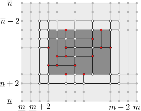
Figure 1: A T-mesh.

The valence of a vertex $V\in\mathsf{V}$ is the number of edges such that $V$ is an endpoint. We only allow valence three (called T-junctions) or four vertices. Note that valence two vertices, other than the four corners, are eliminated from the definition.

The horizontal (resp., vertical) skeleton of a T-mesh is denoted by $h\mathsf{S}$ (resp., $v\mathsf{S}$), and is the union of all horizontal (resp., vertical) edges and all vertices. Finally, we denote the skeleton to be the union $\mathsf{S}=h\mathsf{S}\cup v\mathsf{S}$. For a given vertex $a=\{(i,j)\}$ we define $h\mathsf{J}(a):=\{k\in\mathbb{Z}:\{k\}\times a\subset v\mathsf{S}\}$ and $v\mathsf{J}(a):=\{k\in\mathbb{Z}:a\times\{k\}\subset h\mathsf{S}\}$. We assume that these two sets are ordered.

We split the index domain $\mathsf{R}=[\underline{m},\overline{m}]\times[\underline{n},\overline{n}]$ into an active region $\mathsf{AR}$ and a frame region $\mathsf{FR}$ such that $\mathsf{R}=\mathsf{FR}\cup\mathsf{AR}$ and $\mathsf{AR}=[\underline{m}+2,\overline{m}-2]\times[\underline{n}+2,\overline{n}-2]$, and $\mathsf{FR}=([\underline{m},\underline{m}+2]\cup[\overline{m}-2,\overline{m}])\times[\underline{n},\overline{n}]\cup[\underline{m},\overline{m}]\times([\underline{n},\underline{n}+2]\cup[\overline{n}-2,\overline{n}])$. Note that both $\mathsf{FR}$ and $\mathsf{AR}$ are closed.

A symbolic T-mesh [19] is created from a T-mesh $\mathsf{T}$ by assigning a symbol in Table 1 to each vertex in a tensor product mesh formed from the index coordinates, $\{\underline{m},\ldots,\overline{m}\}\times\{\underline{n},\ldots,\overline{n}\}\subset\mathbb{Z}^{2}$. The symbol is chosen to match the mesh topology of $\mathsf{T}$. The symbolic T-mesh corresponding to the T-mesh in Figure 1 is shown in Figure 2.

Table 1: Definition of possible symbols in a symbolic T-mesh

Symbol	Correspondence with $\mathsf{T}$
$+$	Valence 4 vertex, corner vertex, or valence 3 boundary vertex in $\mathsf{T}$
$\vdash$, $\dashv$, $\bot$, $\top$	Oriented valence three vertex in $\mathsf{T}$
$|$	Vertical edge in $\mathsf{T}$
$-$	Horizontal edge in $\mathsf{T}$
$\cdot$	No corresponding vertex or edge in $\mathsf{T}$

Figure 2: The symbolic representation of the T-mesh in Figure 1.

2.2 Admissible T-meshes

We say that a T-mesh is admissible if it satisfies three basic conditions. First, we require that $\mathsf{S}\cap\mathsf{FR}$ contains the vertical segments $\{i\}\times[\underline{n},\overline{n}]$ for $i=\underline{m},\underline{m}+1,\underline{m}+2,\overline{m}-2,\overline{m}-1,\overline{m}$ and the horizontal segments $[\underline{m},\overline{m}]\times\{j\}$ for $j=\underline{n},\underline{n}+1,\underline{n}+2,\overline{n}-2,\overline{n}-1,\overline{n}$. These horizontal and vertical lines are for basis function definition near the boundary. Second, we require that $\mathsf{S}\cap\mathsf{AR}$ contains the vertical segments $\{i\}\times[\underline{n},\overline{n}]$ for $i=\underline{m}+2,\underline{m}+3,\overline{m}-3,\overline{m}-2$ and the horizontal segments $[\underline{m},\overline{m}]\times\{j\}$ for $j=\underline{n}+2,\underline{n}+3,\overline{n}-3,\overline{n}-2$. Third, we require that for any two vertices $V_{1}=\{(i_{1},j_{1})\},V_{2}=\{(i_{2},j_{2})\}$ in $\mathsf{V}$, such that $V_{1},V_{2}\subset\partial Q$ for some $Q\in\mathsf{T}$, if $i_{1}=i_{2}$ (resp., $j_{1}=j_{2}$), then $\{i_{1}\}\times]j_{1},j_{2}[\subset\mathsf{S}$ (resp., $]i_{1},i_{2}[\times\{j_{1}\}\subset\mathsf{S}$). From a practical point of view these are minor restrictions. The T-mesh in Figure 1 is admissible.

We note that for convenience and simplicity, we often refer to only the active region of an admissible T-mesh when speaking of a T-mesh. In all cases, we assume that the frame region has an admissible topology.

2.3 Anchors and T-junctions

We define the anchors $\mathsf{A}(\mathsf{T})=\{A\in\mathsf{V}\cap\mathsf{AR}\}$. We denote the total number of anchors in $\mathsf{T}$ by $n^{A}$. We define $\mathsf{J}\subset\mathsf{A}(\mathsf{T})$ to be the set of all valence three vertices. These are called T-junctions. The symbols $\vdash$, $\dashv$, $\bot$, $\top$ indicate the four possible orientations of a T-junction in a symbolic T-mesh. A T-junction $T_{h}\in\mathsf{J}$ (resp., $T_{v}\in\mathsf{J}$) of type $\vdash$ and $\dashv$ (resp., $\bot$, $\top$) and their extensions are called horizontal (resp., vertical). The solid white and red circles in Figure 1 are anchors and the red circles are T-junctions.

2.4 Segments

We define a segment to be a closed line segment of contiguous vertices and edges whose beginning and ending vertices are T-junctions (interior or boundary). Given two horizontal (resp., vertical) segments $G_{1}^{h},G_{2}^{h}$ defined over the intervals $[i_{1},j_{1}]\times a$ and $[i_{2},j_{2}]\times b$ we say that $G_{1}^{h}\leq G_{2}^{h}$ if $i_{1}\leq i_{2}$. We denote by $h\mathsf{G}$ (resp., $v\mathsf{G}$) the collection of all horizontal (resp., vertical) segments, and by $\mathsf{G}=h\mathsf{G}\cup v\mathsf{G}$ the collection of all segments. We define $h\mathsf{G}(a)=h\mathsf{G}\cap([\underline{m},\overline{m}]\times a)$ and $v\mathsf{G}(a)=v\mathsf{G}\cap(a\times[\underline{n},\overline{n}])$. We assume these two sets are ordered. We denote the total number of segments in $\mathsf{T}$ by $n^{G}$. We denote the total number of horizontal (resp., vertical) segments in $\mathsf{T}$ by $n^{G}_{h}$ (resp., $n^{G}_{v}$). We denote the number of line segments in $h\mathsf{G}(a)$ (resp., $v\mathsf{G}(a)$) by $n^{G}_{h}(a)$ (resp., $n^{G}_{v}(a)$).

2.5 The extended T-mesh

T-junction extensions can be associated with each T-junction. For example, given a T-junction $T=\{(\overline{\imath},\overline{\jmath})\}\in\mathsf{J}$ of type $\vdash$ we extract from $h\mathsf{J}(\{\overline{\jmath}\})$ four consecutive indices $i_{1},\ldots,i_{4}$ such that $\overline{\imath}=i_{3}$. We call $ext^{e}(T)=[i_{1},\overline{\imath}]\times\{\overline{\jmath}\}$ the face extension, $ext^{f}(T)=]\overline{\imath},i_{4}]\times\{\overline{\jmath}\}$ the edge extension for such kind of T-junction. Similarly, we can define the face and edge extensions for the other kinds of T-junctions $\dashv$, $\bot$, $\top$ which are illustrated in Figure 3.

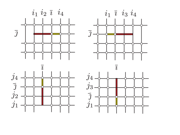
Figure 3: The face extension (red) and edge extension (yellow) for four different kinds of T-junctions.

We denote $ext(T)=ext^{e}(\mathsf{T})\cup ext^{f}(T)$ the extension of T-junction $T$ and the union of all horizontal (resp., vertical) face extensions by $hext^{f}(\mathsf{T})$ (resp., $vext^{f}(\mathsf{T})$), the union of all face extensions by $ext^{f}(\mathsf{T})$, and the union of all extensions (face and edge) by $ext(\mathsf{T})$. We define the extended T-mesh, $\mathsf{T}_{ext}$, as the T-mesh created by adding to $\mathsf{T}$ all the T-junction extensions. In other words, $\mathsf{T}_{ext}=\mathsf{T}\cup ext(\mathsf{T})$. We denote the total number of vertices in $\mathsf{T}_{ext}$ by $n^{ext}$. The extended T-mesh corresponding to the T-mesh in Figure 1 is shown in Figure 4.

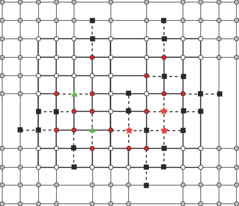
Figure 4: The extended T-mesh corresponding to the T-mesh in Figure 1. The crossing vertices are denoted by red stars, the overlap vertices are denoted by green triangles, and the extended vertices are denoted by black squares. Notice that the inactive vertices (grey circles) are also regarded as extended vertices. The active vertices are denoted by hollow circles and the T-junctions are denoted by red circles.

Adding T-junction extensions to $\mathsf{T}$ may introduce three additional collections of vertices. The first, called crossing vertices and denoted by $\mathsf{CV}$, is created from the intersection of crossing face extensions. In other words,

$$\mathsf{CV}=hext(\mathsf{T})\cap vext(\mathsf{T}).$$

We denote the number of crossing vertices in $\mathsf{T}_{ext}$ by $n^{+}$. In Figure 4 the crossing vertices are denoted by red stars.

The second, called overlap vertices and denoted by $\mathsf{OV}$, is created from the intersection of overlapping face extensions with $\mathsf{S}$. In other words,

$$\mathsf{OV}=((\bigcap_{T_{h}\in\mathsf{J}}ext^{f}(T_{h}))\cap v\mathsf{S})\cup((\bigcap_{T_{v}\in\mathsf{J}}ext^{f}(T_{v}))\cap h\mathsf{S}).$$

We denote the number of overlap vertices in $\mathsf{T}_{ext}$ by $n^{-}$. In Figure 4 the overlap vertices are denoted by green triangles.

The third, called extended vertices and denoted by $\mathsf{EV}$, is created from the intersection of face extensions and $\mathsf{S}$ while removing those vertices which already correspond to overlap vertices. Additionally, all non-anchor vertices are classified as extended vertices. In other words,

$$\mathsf{EV}=((ext^{f}(\mathsf{T})\cap\mathsf{S})\setminus\mathsf{OV})\cup(\mathsf{V}\setminus\mathsf{A}(\mathsf{T})).$$

We denote the number of extended vertices in $\mathsf{T}_{ext}$ by $n^{*}$. In Figure 4 the extended vertices are denoted by black squares.

3 The parametric domain and T-spline spaces

Let $\Xi=(\xi_{\underline{m}},\ldots,\xi_{\overline{m}})$ and $\Pi=(\eta_{\underline{n}},\ldots,\eta_{\overline{n}})$ be two global knot vectors defined on the interval $\mathbb{R}$. Interior knots may have a multiplicity of three while end knots may have a multiplicity of four. The global knot vectors define a full parametric domain, $\tilde{\Omega}\subset\mathbb{R}^{2}$, where $\tilde{\Omega}=[\xi_{\underline{m}},\xi_{\overline{m}}]\otimes[\eta_{\underline{n}},\eta_{\overline{n}}]$ and a reduced parametric domain, $\hat{\Omega}\subset\tilde{\Omega}$, where $\hat{\Omega}=[\xi_{\underline{m}+3},\xi_{\overline{m}-3}]\otimes[\eta_{\underline{n}+3},\eta_{\overline{n}-3}]$. The T-mesh in the parametric domain is defined as the collection of non-empty elements of the form $\tilde{Q}=]\xi_{i_{1}},\xi_{i_{2}}[\times]\eta_{j_{1}},\eta_{j_{2}}[$ where $Q=]i_{1},i_{2}[\times]j_{1},j_{2}[\in\mathsf{T}$. We denote those elements where $\tilde{Q}\cap\hat{\Omega}\neq\emptyset$ by $\hat{Q}$. The extended T-mesh in the parametric domain as well as all element related concepts are defined similarly. Throughout this paper we use the index and parametric representation of a T-mesh interchangeably with the context making the use clear.

For each anchor $A=a\times b\in\mathsf{A}(\mathsf{T})$ we define its horizontal (vertical) index vector $hv(A)$ ($vv(A)$, respectively) as a subset of $h\mathsf{J}(b)$ ($v\mathsf{J}(a)$, respectively) where $hv(A)=(i_{1},\ldots,i_{5})\in\mathbb{Z}^{5}$ contains five unique consecutive indices in $h\mathsf{J}(b)$ with $\{i_{3}\}=a$. The vertical index vector, denoted by $vv(A)$, is constructed in an analogous manner. We then associate a T-spline blending function $N_{A}(\xi,\eta)$ with anchor $A$. The T-spline blending functions are given by

$$N_{A}(\xi,\eta):=B[\Xi_{A}](\xi)B[\Pi_{A}](\eta)\quad\forall(\xi,\eta)\in\hat{\Omega}$$ (1)

where $B[\Xi_{A}](\xi)$ and $B[\Pi_{A}](\eta)$ are the cubic B-spline basis functions associated with the local knot vectors

$$\Xi_{A} =[\xi_{i_{1}},\ldots,\xi_{i_{5}}]\subset\Xi$$ (2)

$$\Pi_{A} =[\eta_{j_{1}},\ldots,\eta_{j_{5}}]\subset\Pi$$ (3)

and $hv(A)=(i_{1},\ldots,i_{5})$ and $vv(A)=(j_{1},\ldots,j_{5})$.

Figure 5 illustrates the construction of a T-spline blending function corresponding to anchor $A=\{(3,3)\}$. In this case, the local knot vectors are $\Xi_{A}=[\xi_{1},\xi_{2},\xi_{3},\xi_{4},\xi_{6}]$ and $\Pi_{A}=[\eta_{1},\eta_{2},\eta_{3},\eta_{4},\eta_{5}]$.

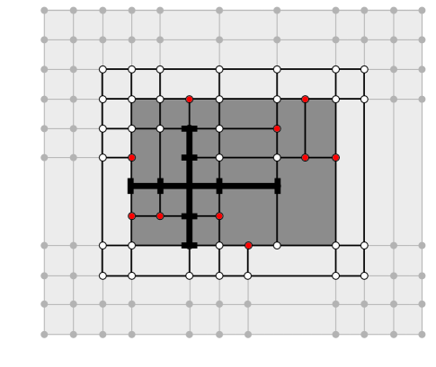
Figure 5: Inferring a T-spline blending function from a T-mesh.

A T-spline space $\mathcal{T}=\mathcal{T}(\mathsf{T},\Xi,\Pi)$ is simply the span of the blending functions, $N_{A}$, $A\in\mathsf{A}(\mathsf{T})$.

4 Analysis-suitable T-splines

Analysis-suitable T-splines form a practically useful subset of T-splines. ASTS maintain the important mathematical properties of the NURBS basis while providing an efficient and highly localized refinement capability. Several important properties of ASTS have been proven:

• The blending functions are linearly independent for any choice of knots [19].

• The basis constitutes a partition of unity (see Corollary 6.7).

• Each basis function is non-negative.

• They can be generalized to arbitrary degree [21].

• An affine transformation of an analysis-suitable T-spline is obtained by applying the transformation to the control points. We refer to this as affine covariance. This implies that all “patch tests” (see [23]) are satisfied a priori.

• They obey the convex hull property.

• They can be locally refined [1, 3].

• A dual basis can be constructed [20, 21].

Definition 4.1.

An analysis-suitable T-spline is a T-spline whose T-mesh is analysis-suitable [19]. A T-mesh is said to be analysis-suitable if it is admissible and no horizontal T-junction extension intersects a vertical T-junction extension.

An analysis-suitable T-mesh is shown in Figure 6a. The corresponding extended T-mesh is shown in Figure 6b. Notice that no horizontal extension intersects a vertical extension. The dual basis for an ASTS equips these spaces with a rich mathematical structure which we leverage in this paper [20].

Lemma 4.2.

For a bicubic ASTS, each dual basis function, corresponding to a T-spline basis function $N_{A}(\xi,\eta)$ with local knot vectors $\Xi_{A}=[\xi_{i_{1}},\ldots,\xi_{i_{5}}]$ and $\Pi_{A}=[\eta_{j_{1}},\ldots,\eta_{j_{5}}]$, is

$$\lambda_{A}=\lambda[\xi_{i_{1}},\ldots,\xi_{i_{5}}]\otimes\lambda[\eta_{j_{1}},\ldots,\eta_{j_{5}}]$$

where $\lambda[\xi_{i_{1}},\ldots,\xi_{i_{5}}]$ and $\lambda[\eta_{j_{1}},\ldots,\eta_{j_{5}}]$ are dual basis functions corresponding to univariate cubic B-splines [24] whose knot vectors are $[\xi_{i_{1}},\ldots,\xi_{i_{5}}]$ and $[\eta_{j_{1}},\ldots,\eta_{j_{5}}]$, respectively.

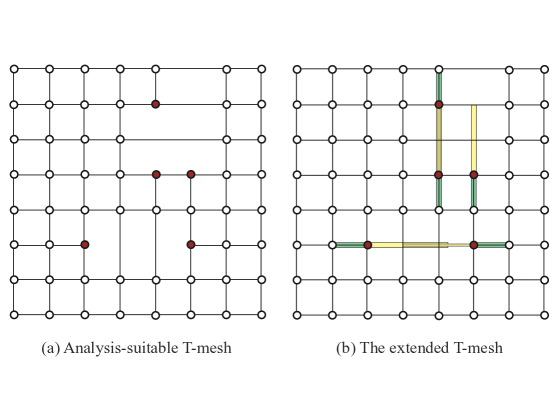
Figure 6: An analysis-suitable T-mesh (a) and the extended T-mesh (b).

5 Perturbed T-splines

From a theoretical point of view, developing a complete and rigorous characterization of T-spline spaces is complicated by the presence of zero knot intervals (especially near T-junctions) and overlap vertices. However, allowing both is important when T-splines are used as a tool in design and analysis.

To overcome this difficulty, we develop the theory of the perturbed T-mesh (and resulting perturbed T-spline space). A perturbed T-spline can be used to prove properties about the original T-spline. In other words, we will generate a perturbed T-mesh, establish the result in the perturbed setting, and then show that the result holds as the perturbation converges to the original T-spline.

5.1 Perturbed T-meshes

A perturbed T-mesh is created by first generating perturbed global knot vectors, $\Xi[\boldsymbol{\delta}]$, $\Pi[\boldsymbol{\delta}]$, where $\boldsymbol{\delta}=(\delta_{1},\ldots,\delta_{n})^{T}$ is a vector of perturbation parameters. A perturbed global knot vector is written as

$$\Xi[\boldsymbol{\delta}]=(\xi[\boldsymbol{\delta}]_{\underline{\imath}},\ldots,\xi[\boldsymbol{\delta}]_{\imath},\ldots,\xi[\boldsymbol{\delta}]_{\overline{\imath}})$$

where $\imath=\imath(i,g)$ takes the index of the $i^{th}$ knot in $\Xi$ and the $g^{th}$ segment in $v\mathsf{G}(\{i\})$ and returns a unique index in the perturbed global knot vector. The knot values are initialized as $\xi[\boldsymbol{\delta}]_{\imath(i,g)}=\xi_{i}$. In other words, a knot index which corresponds to a $v\mathsf{G}(\{i\})$ which contains multiple segments in the T-mesh is repeated $n_{v}^{G}(\{i\})$ times. Notice that this operation induces an index map $h\pi(\imath(i,g))=i$ (resp., $v\pi$) from the indices in the perturbed global knot vector onto the original global knot vector. The knot values are then perturbed using a small parameter $\delta\in\mathbb{R}$ as

$$\xi[\boldsymbol{\delta}]_{\imath}=\xi[\boldsymbol{\delta}]_{\underline{\imath}}+\sum_{\jmath=\underline{\imath}+1}^{\imath}\Delta\xi[\boldsymbol{\delta}]_{\jmath},\quad\imath=\underline{\imath},\ldots,\overline{\imath}$$

where $\Delta\xi[\boldsymbol{\delta}]_{\jmath}=c_{\alpha(\jmath)}\delta=\delta_{\alpha}$, if $\xi_{h\pi(\jmath)}-\xi_{h\pi({\jmath}-1)}=0$, and is equal to $\xi_{h\pi(\jmath)}-\xi_{h\pi({\jmath}-1)}$, otherwise. The constant, $c_{\alpha}\in[0,\infty)$. This same procedure is applied to $\Pi$ to form $\Pi[\boldsymbol{\delta}]$. The T-mesh, $\mathsf{T}$, is then modified to form the perturbed T-mesh, $\mathsf{T}[\boldsymbol{\delta}]$, by associating the vertices and edges contained in the $g^{th}$ segment of $v\mathsf{G}(\{i\})$ with knot $\xi[\boldsymbol{\delta}]_{\imath(i,g)}$. Notice that the number of anchors does not change when forming $\mathsf{T}[\boldsymbol{\delta}]$. A perturbed T-spline space $\mathcal{T}[\boldsymbol{\delta}]$ is a T-spline space formed from perturbed global knot vectors and T-mesh. A strictly perturbed T-mesh or T-spline space is one where $c_{\alpha}\in(0,\infty)$.

A perturbation of an analysis-suitable T-mesh is shown in Figure 7. The analysis-suitable T-mesh is shown in Figure 7a and the perturbed T-mesh is shown in Figure 7b. Knot intervals are shown instead of knots for simplicity. Recall that a knot interval is simply the difference between adjacent knots in a global knot vector. Notice that the horizontal and vertical zero knot intervals have been replaced by non-zero knot intervals $\sigma_{2}$ and $\sigma_{3}$. The vertical segments with T-junctions are perturbed resulting in a new knot interval $\sigma_{1}$.

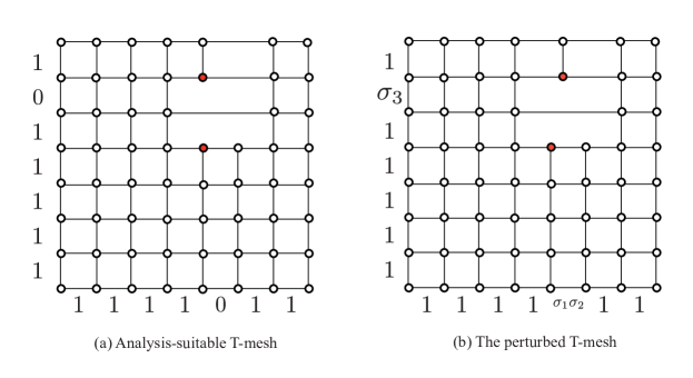
Figure 7: A perturbation of an analysis-suitable T-mesh $\mathsf{T}$ shown in (a) results in the perturbed T-mesh $\mathsf{T}[\boldsymbol{\delta}]$ shown in (b).

Proposition 5.1.

If $\mathsf{T}$ is analysis-suitable then $\mathsf{T}[\boldsymbol{\delta}]$ is analysis-suitable.

Proof.

Suppose the extensions of two T-junctions $ext(V_{1})=[i_{1}^{1},i_{4}^{1}]\times\{j^{1}\}$ ($\vdash$ or $\dashv$) and $ext(V_{2})=\{i^{2}\}\times[j_{1}^{2},j_{4}^{2}]$ ($\bot$ or $\top$) in $\mathsf{T}[\boldsymbol{\delta}]$ intersect. This implies that $j_{1}^{2}\leq j^{1}\leq j_{4}^{2}$ and $i_{1}^{1}\leq i^{2}\leq i_{4}^{1}$. According to the construction of $\mathsf{T}[\boldsymbol{\delta}]$, we don’t change the order of the indices, so $h\pi(j_{1}^{2})\leq h\pi(j^{1})\leq h\pi(j_{4}^{2})$ and $v\pi(i_{1}^{1})\leq v\pi(i^{2})\leq v\pi(i_{4}^{1})$, i.e., there are intersecting extensions in $\mathsf{T}$. ∎

Lemma 5.1.

Let $\mathsf{T}$ be an analysis-suitable T-mesh. For every anchor, $\{(\imath,\jmath)\}$, and horizontal index vector, $hv(\{(\imath,\jmath)\})[\boldsymbol{\delta}]$, in the perturbed T-mesh, $\mathsf{T}[\boldsymbol{\delta}]$, $hv(\{(h\pi(\imath),v\pi(\jmath))\})=h\pi(hv(\{(\imath,\jmath)\})[\boldsymbol{\delta}])$ where $h\pi(hv(\{(\imath,\jmath)\})[\boldsymbol{\delta}])=(h\pi(\imath_{1}),\ldots,h\pi(\imath_{5}))$. This also holds for the vertical index vectors.

Proof.

If the topological symbols corresponding to the indices $\{(i_{1},\jmath),\ldots,(i_{5},\jmath)\}$ where $i_{\ell}\in hv(\{(\imath,\jmath)\})[\boldsymbol{\delta}]$, $\ell=1,\ldots,5$, are not $\vdash$ or $\dashv$ then the result immediately follows since the indices are contained in a single horizontal segment. Thus, we only need to prove that the result holds when the topological symbol corresponding to $\{(\imath,\jmath)\}$ is $\vdash$ or $\dashv$. Without loss of generality we assume it to be $\vdash$. Since, according to Lemma 5.1, the T-mesh, $\mathsf{T}[\boldsymbol{\delta}]$, is analysis-suitable the symbols for the first two indices in $hv(\{(\imath,\jmath)\})[\boldsymbol{\delta}]$ can only be $|$ or $\dashv$. Thus, $hv(\{(h\pi(\imath),v\pi(\jmath))\})=h\pi(hv(\{(\imath,\jmath)\})[\boldsymbol{\delta}])$. ∎

Theorem 5.2.

If $\mathcal{T}$ is analysis-suitable and $\mathcal{T}[\boldsymbol{\delta}]$ is an offset perturbation then $N_{A}[\boldsymbol{\delta}]\rightarrow N_{\pi(A)}$ as $\delta\rightarrow 0$, $A\in\mathsf{A}(\mathsf{T}[\boldsymbol{\delta}])$ where $\pi(A)=\{(h\pi(\imath),v\pi(\jmath))\}$.

Proof.

Notice that if $\delta\rightarrow 0$, $\xi[\boldsymbol{\delta}]_{\imath}\rightarrow\xi_{h\pi(\imath)}$ for any $\imath$ and $\eta[\delta]_{\jmath}\rightarrow\eta_{v\pi(\jmath)}$ for any $\jmath$. According to Lemma 5.1, the local knot vectors for each basis function $N_{A}[\boldsymbol{\delta}]$ converge to those for $N_{\pi(A)}$, $A\in\mathsf{A}(\mathsf{T}[\boldsymbol{\delta}])$. Thus, according to ([24], Theorem 4.36) we have the result. ∎

6 Refineability and nestedness

We now explore the refineability and nesting behavior of analysis-suitable T-spline spaces. In other words, given two analysis-suitable T-splines spaces, $\mathcal{T}^{1}$ and $\mathcal{T}^{2}$, we establish the conditions under which $\mathcal{T}^{1}\subseteq\mathcal{T}^{2}$. We first establish basic refineability properties when the analysis-suitable T-mesh does not have any knot multiplicities or overlap vertices. Using the theory of perturbed T-splines, we then extend those results to encompass T-meshes which do have zero knot intervals and overlap vertices.

Definition 6.1.

The notation $\mathsf{T}^{1}[\boldsymbol{\delta},\mathsf{T}^{2}]$ denotes a perturbed T-mesh where $\mathsf{T}^{1}\subseteq\mathsf{T}^{2}$ and $\mathsf{T}^{1}[\boldsymbol{\delta},\mathsf{T}^{2}]$ is created by removing those edges and vertices from the strictly perturbed T-mesh $\mathsf{T}^{2}[\boldsymbol{\delta}]$ which correspond to unperturbed edges and vertices in $\mathsf{T}^{2}\setminus\mathsf{T}^{1}$. By inspection, it is clear that $\mathsf{T}^{1}[\boldsymbol{\delta},\mathsf{T}^{2}]$, constructed in this way, is a perturbed T-mesh which satisfies Proposition 5.1, Lemma 5.1, and Theorem 5.2 and that $\mathsf{T}^{1}[\boldsymbol{\delta},\mathsf{T}^{2}]\subseteq\mathsf{T}^{2}[\boldsymbol{\delta}]$.

The construction of $\mathsf{T}^{1}[\boldsymbol{\delta},\mathsf{T}^{2}]$ is depicted in Figure 8. Two analysis-suitable T-meshes are shown in Figure 8a and Figure 8b. Notice that $\mathsf{T}^{1}\subseteq\mathsf{T}^{2}$. The perturbed T-mesh $\mathsf{T}^{1}[\boldsymbol{\delta},\mathsf{T}^{2}]$ (shown in Figure 8c) is formed by removing the dotted lines (shown in Figure 8c) from $\mathsf{T}^{2}[\boldsymbol{\delta}]$ (shown in Figure 8d).

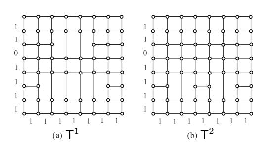
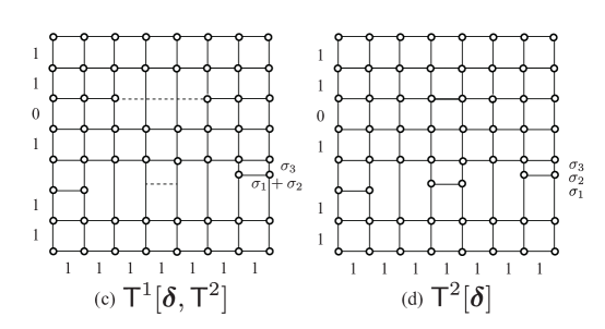
Figure 8: The construction of $\mathsf{T}^{1}[\boldsymbol{\delta},\mathsf{T}^{2}]$. Two analysis-suitable T-meshes are shown in (a) and (b) such that $\mathsf{T}^{1}\subseteq\mathsf{T}^{2}$. The perturbed T-mesh $\mathsf{T}^{1}[\boldsymbol{\delta},\mathsf{T}^{2}]$, shown in (c), is formed by removing the dotted lines from $\mathsf{T}^{2}[\boldsymbol{\delta}]$, shown in (d).

Definition 6.2.

Given a T-mesh, $\mathsf{T}$, with no knot multiplicities, and the corresponding extended T-mesh, $\mathsf{T}_{ext}$, the homogeneous extended spline space is defined as

$$\mathcal{S}_{ext}=\left\{f\in C^{2,2}(\mathbb{R}^{2})\,|\,f|_{\tilde{Q}_{ext}}\in\mathbb{P}_{33},\forall\tilde{Q}_{ext}\subseteq\tilde{\Omega},\,\mathrm{and}\,f|_{\mathbb{R}^{2}\setminus\tilde{\Omega}}\equiv 0\right\}$$ (4)

where $C^{2,2}(\mathbb{R}^{2})$ is the space of bivariate functions which are $C^{2}$-continuous in $\xi$ and $\eta$ over all of $\mathbb{R}^{2}$. $\mathbb{P}_{33}$ is the space of bicubic polynomials. The extended spline space is defined to be $\mathcal{T}_{ext}=\mathcal{S}_{ext}|_{\hat{\Omega}}$.

Proposition 6.1.

$\dim\mathcal{T}_{ext}=\dim\mathcal{S}_{ext}$

Proof.

We first prove that the dimension of $\mathcal{S}_{ext}$ is not less than the dimension of $\mathcal{T}_{ext}$. Notice that for any function $f\in\mathcal{S}_{ext}$, $f|_{\hat{\Omega}}\in\mathcal{T}_{ext}$. We now show that the dimension of $\mathcal{T}_{ext}$ is not less than the dimension of $\mathcal{S}_{ext}$. This is equivalent to showing that there is only one function in $\mathcal{S}_{ext}$ which is zero over $\hat{\Omega}$. It is easy to see that the only function which is zero over $\hat{\Omega}$ must be zero over all of $\mathbb{R}^{2}$ since the minimum support of a cubic $C^{2}$ spline function is four intervals. ∎

Lemma 6.3.

If the extended T-mesh, $\mathsf{T}_{ext}$, of an analysis-suitable T-mesh, $\mathsf{T}$, has no knot multiplicities or overlap vertices, then $\mathcal{T}=\mathcal{T}_{ext}$. In other words, the analysis-suitable T-spline space, $\mathcal{T}$, and the extended spline space, $\mathcal{T}_{ext}$, are the same space.

Proof.

We have that $\mathcal{T}\subseteq\mathcal{T}_{ext}$ (see [20], Lemma 4.3), so the dimension of $\mathcal{T}$ is less than that of $\mathcal{T}_{ext}$, which, according to Theorem 8.5, Proposition 6.1, and Theorem 8.9 is the number of active vertices. Since the blending functions for anaysis-suitable T-splines are linearly independent the dimension of $\mathcal{T}$ is also the number of active vertices. Thus, the two spline spaces are identical. ∎

Lemma 6.4.

Given two analysis-suitable T-meshes, $\mathsf{T}^{1}$ and $\mathsf{T}^{2}$, neither of which has knot multiplicities or overlap vertices, if $\mathsf{T}_{ext}^{1}\subseteq\mathsf{T}_{ext}^{2}$, then $\mathcal{T}^{1}\subseteq\mathcal{T}^{2}$.

Proof.

Obviously, $\mathcal{T}_{ext}^{1}\subseteq\mathcal{T}_{ext}^{2}$. Since $\mathsf{T}^{1}$ and $\mathsf{T}^{2}$ are analysis-suitable, according to Lemma 6.3, $\mathcal{T}^{1}\subseteq\mathcal{T}^{2}$. ∎

Lemma 6.5.

Given two analysis-suitable T-spline spaces, $\mathcal{T}^{1}$ and $\mathcal{T}^{2}$, if $\mathcal{T}^{1}[\boldsymbol{\delta}]\subseteq\mathcal{T}^{2}[\boldsymbol{\delta}]$, then $\mathcal{T}^{1}\subseteq\mathcal{T}^{2}$.

Proof.

Suppose the perturbed T-spline space, $\mathcal{T}^{1}[\boldsymbol{\delta}]$, is spanned by the basis functions, $N_{A}^{1}[\boldsymbol{\delta}]$, and the perturbed T-spline space, $\mathcal{T}^{2}[\boldsymbol{\delta}]$, is spanned by the basis functions, $N_{B}^{2}[\boldsymbol{\delta}]$. We have that

$$N_{A}^{1}[\boldsymbol{\delta}]=\sum\lambda_{B}(N_{A}[\boldsymbol{\delta}])N_{B}^{2}[\boldsymbol{\delta}].$$

where $\lambda_{B}$, $B\in\mathsf{A}(\mathsf{T}^{2}[\boldsymbol{\delta}])$ are the dual functionals for the analysis-suitable T-spline basis $N_{B}[\boldsymbol{\delta}]$ as described in [20]. According to Theorem 5.2,

$$\lim_{\delta\rightarrow 0}N_{B}^{2}[\boldsymbol{\delta}]=N_{\pi(B)}^{2},\quad\lim_{\delta\rightarrow 0}N_{A}^{1}[\boldsymbol{\delta}]=N_{\pi(A)}^{1}.$$

According to Theorem 4.41 in [24], $\lambda_{B}(N_{A}[\boldsymbol{\delta}])$ is bounded, so

$$\lim_{\delta\rightarrow 0}\lambda_{B}(N_{A}[\boldsymbol{\delta}])=c_{B}^{A},$$

i.e.,

$$N_{\pi(A)}^{1}=\sum c_{B}^{A}N_{\pi(B)}^{2}.$$

∎

Theorem 6.6.

Given two analysis-suitable T-meshes, $\mathsf{T}^{1}$ and $\mathsf{T}^{2}$, if $\mathsf{T}^{1}_{ext}[\boldsymbol{\delta},\mathsf{T}^{2}]\subseteq\mathsf{T}^{2}_{ext}[\boldsymbol{\delta}]$, then $\mathcal{T}^{1}\subseteq\mathcal{T}^{2}$.

Proof.

Obviously, $\mathcal{T}_{ext}^{1}[\boldsymbol{\delta},\mathsf{T}^{2}]\subseteq\mathcal{T}_{ext}^{2}[\boldsymbol{\delta}]$. Since $\mathsf{T}_{ext}^{2}[\boldsymbol{\delta}]$ has no knot multiplicities or overlap vertices we have that $\mathcal{T}^{2}[\boldsymbol{\delta}]=\mathcal{T}^{2}_{ext}[\boldsymbol{\delta}]$ according to Lemma 6.3. Since the extended T-mesh, $\mathsf{T}^{1}_{ext}[\boldsymbol{\delta},\mathsf{T}^{2}]$, may have overlap vertices but no knot multiplicities we have that $\mathcal{T}^{1}[\boldsymbol{\delta},\mathsf{T}^{2}]\subseteq\mathcal{T}^{1}_{ext}[\boldsymbol{\delta},\mathsf{T}^{2}]$ according to Theorem 8.5 and Proposition 6.1. This immediately implies that $\mathcal{T}^{1}\subseteq\mathcal{T}^{2}$. ∎

Proposition 6.2.

Every analysis-suitable T-spline space contains the space of bicubic polynomials.

Proof.

We have that any bicubic polynomial $f[\boldsymbol{\delta}]\in\mathcal{T}[\boldsymbol{\delta}]$ according to Lemma 6.3. Using the dual basis for $\mathcal{T}[\boldsymbol{\delta}]$ we have that

$$f[\boldsymbol{\delta}]=\sum\lambda_{A}(f)N_{A}[\boldsymbol{\delta}].$$

Thus, according to Theorem 5.2 and ([24], Theorem 4.41), as $\delta\rightarrow 0$,

$$f=\sum c_{A}N_{A}.$$

∎

Corollary 6.7.

Every analysis-suitable T-spline space forms a partition of unity. In other words, $\sum_{A}N_{A}(\xi,\eta)=1$, $\forall(\xi,\eta)\in\hat{\Omega}$.

Proof.

This immediately follows from Proposition 6.2 and the fact that $\lambda_{A}(1)=1$. ∎

7 Approximation

As described in [20, 21] approximation properties of analysis-suitable T-splines are directly linked to Proposition 6.2. In other words, having the bicubic polynomials in the T-spline space is the minimal requirement to obtain an $O(h^{4})$ convergence rate in the mesh size.

Following the approach in [22, 20, 21], the dual basis for an analysis-suitable T-spline space, $\mathcal{T}$, can be used to construct a projection operator, $\mathbb{P}:L^{2}(\hat{\Omega})\rightarrow\mathcal{T}$, where

$$\mathbb{P}(f)(\xi,\eta)=\sum_{A\in\mathsf{A}(\mathsf{T})}\lambda_{A}(f)N_{A}(\xi,\eta)\quad\forall f\in L^{2}(\hat{\Omega}),\forall(\xi,\eta)\in\hat{\Omega}.$$

We denote the open support of a T-spline basis function by $Q_{A}\subset\tilde{\Omega}$, and the extended support of an element $\hat{Q}$ by $\Omega_{\hat{Q}}\subset\tilde{\Omega}$, where

$$\Omega_{\hat{Q}}=\bigcup_{A\in\mathsf{A}(\hat{Q})}Q_{A},\quad\mathsf{A}(\hat{Q})=\{A\in\mathsf{A}(\mathsf{T}):Q_{A}\cap\hat{Q}\neq\emptyset\}.$$

We will denote by $R(\Omega_{\hat{Q}})$ the smallest rectangle in $\tilde{\Omega}$ containing $\Omega_{\hat{Q}}$ and .

Proposition 7.1.

Given an analysis-suitable T-spline space, $\mathcal{T}$, the projection operator $\mathbb{P}$ is (locally) h–uniformly continuous in the $L^{2}$ norm. In other words, there exists a constant $C$ independent of $\mathsf{T},\Xi,\Pi$ such that

$$||\mathbb{P}(f)||_{L^{2}(\hat{Q})}\leq C||f||_{L^{2}(\Omega_{\hat{Q}})}\quad\forall\hat{Q}\in\mathsf{T}_{ext},\forall f\in L^{2}(\hat{\Omega})$$

Note that the constant $C$ may depend on the polynomial degree.

Proof.

The result follows immediately from ([20], Proposition 5.4) and Proposition 6.2. ∎

Proposition 7.2.

Given an analysis-suitable T-spline space, $\mathcal{T}$, there exists a constant $C^{\prime}$ independent of $\mathsf{T},\Xi,\Pi$ such that for $r\in[0,4]$

$$||f-\mathbb{P}(f)||_{L^{2}(\hat{Q})}\leq C^{\prime}(h_{R(\Omega_{\hat{Q}})})^{r}|f|_{H^{r}(R(\Omega_{\hat{Q}}))}\quad\forall\hat{Q}\in\mathsf{T}_{ext},\forall f\in L^{2}(\hat{\Omega})$$

where $h_{R(\Omega_{\hat{Q}})}$ denotes the diameter of $R(\Omega_{\hat{Q}})$. Note that the constant $C^{\prime}$ may depend on the polynomial degree.

Proof.

The result follows immediately from ([20], Proposition 5.4) and Proposition 6.2. ∎

8 Dimension

In this section, we develop a dimension formula for polynomial spline spaces defined over the extended T-mesh in the parametric domain of a T-spline and establish the connection between this dimension formula and analysis-suitable T-spline spaces. The dimension formula, written only in terms of topological quantities of the original T-mesh, is an essential ingredient in establishing the refineability properties in Section 6 and the approximation results in Section 7 for analysis-suitable T-splines. The essential results are proven in Theorems 8.5 and 8.9.

Unlike existing approaches, our dimension formula does not require that the T-mesh have any nesting structure. Of critical importance is how this dimension formula can be directly related to analysis-suitable T-spline spaces which can then be used to construct a simple set of basis functions for the spline space which are compatible with commercial CAD and analysis frameworks.

8.1 Smoothing cofactor-conformality method

We use the smoothing cofactor-conformality method [25, 24] to transform the smoothness properties of $\mathcal{S}_{ext}$ into a linear constraint matrix, $\mathbf{M}$. This constraint matrix is then analyzed to determine the dimension of $\mathcal{S}_{ext}$. We recall that the spline space, $\mathcal{S}_{ext}$, is defined using the extended T-mesh, $\mathsf{T}_{ext}$, corresponding to a T-mesh, $\mathsf{T}$, which does not have any knot multiplicities.

8.1.1 Vertex and edge cofactors

As shown in Figure 9, for any vertex, $V_{i,j}=(\xi_{i},\eta_{j})\in\mathsf{T}_{ext}$, the surrounding bicubic polynomial patches are labeled, $p_{i,j}^{k}(\xi,\eta)$, $k=0,1,2,3$. If the vertex, $V_{i,j}$, is a T-junction, then $p_{i,j}^{k}(\xi,\eta)=p_{i,j}^{k+1}(\xi,\eta)$ for some $k$. Since $p_{i,j}^{0}(\xi,\eta)$ and $p_{i,j}^{1}(\xi,\eta)$ are $C^{2}$-continuous there exists a cubic polynomial $\gamma_{i,j}^{2}(\eta)$, called the edge cofactor, such that

$$p_{i,j}^{1}(\xi,\eta)-p_{i,j}^{0}(\xi,\eta)=\gamma_{i,j}^{2}(\eta)(\xi-\xi_{i})^{3}.$$ (5)

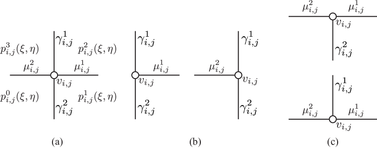
Figure 9: The smoothing cofactors around a vertex.

Similarly, there exists cubic polynomials, $\gamma_{i,j}^{1}(\eta)$, $\mu_{i,j}^{1}(\xi)$, and $\mu_{i,j}^{2}(\xi)$, such that

$$p_{i,j}^{2}(\xi,\eta)-p_{i,j}^{1}(\xi,\eta) =\mu_{i,j}^{1}(\xi)(\eta-\eta_{j})^{3},$$ (6)

$$p_{i,j}^{3}(\xi,\eta)-p_{i,j}^{2}(\xi,\eta) =-\gamma_{i,j}^{1}(\eta)(\xi-\xi_{i})^{3},$$ (7)

$$p_{i,j}^{0}(\xi,\eta)-p_{i,j}^{3}(\xi,\eta) =-\mu_{i,j}^{2}(\xi)(\eta-\eta_{j})^{3}.$$ (8)

We note that if two patches are identical the edge cofactor is zero. Combining (5) - (8) gives

$$(\gamma_{i,j}^{1}(\eta)-\gamma_{i,j}^{2}(\eta))(\xi-\xi_{i})^{3}=(\mu_{i,j}^{1}(\xi)-\mu_{i,j}^{2}(\xi))(\eta-\eta_{j})^{3}.$$ (9)

Since $(\xi-\xi_{i})^{3}$ and $(\eta-\eta_{j})^{3}$ are prime to each other there exists a constant, $d_{i,j}$, called the vertex cofactor, such that

$$\gamma_{i,j}^{1}(\eta)-\gamma_{i,j}^{2}(\eta)=d_{i,j}(\eta-\eta_{j})^{3},\quad\mu_{i,j}^{1}(\xi)-\mu_{i,j}^{2}(\xi)=d_{i,j}(\xi-\xi_{i})^{3}.$$ (10)

8.1.2 Assembling the constraint matrix, $\mathbf{M}$

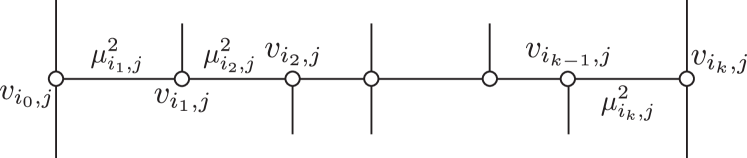
Figure 10: The smoothing cofactors along a horizonal edge segment.

Referring to Figure 10, consider a horizontal segment $G_{j}^{h}$ with $k+1$ vertices and $k$ edge cofactors. Using (10) we have that

$$\mu_{i_{0},j}^{1}-0 =d_{i_{0},j}(\xi-\xi_{i_{0}})^{3},$$ (11)

$$\mu_{i_{1},j}^{2}-\mu_{i_{1},j}^{1} =d_{i_{1},j}(\xi-\xi_{i_{1}})^{3},$$ (12)

$$\,\,\,\vdots$$

$$0-\mu_{i_{k},j}^{2} =d_{i_{k},j}(\xi-\xi_{i_{k}})^{3},$$ (13)

and

$$\mu_{i_{\ell+1},j}^{2}=\mu_{i_{\ell},j}^{1},\,\,\ell=1,\ldots,k.$$ (14)

Summing (11) - (13) and using (14) results in the linear system

$$L_{j}^{h}:=\sum_{\ell=0}^{k}d_{i_{\ell},j}(\xi-\xi_{i_{\ell}})^{3}=0.$$ (15)

We call the solution space, denoted by $W[G_{j}^{h}]$, for this linear system the edge conformality space. Similarly, for a vertical segment $G_{i}^{v}$ we have that

$$L_{i}^{v}:=\sum_{\ell=0}^{l}d_{i,j_{\ell}}(\eta-\eta_{j_{\ell}})^{3}=0$$ (16)

where the solution space is denoted by $W[G_{i}^{v}]$. By (15) and (16), one immediately has that

Lemma 8.1.

If each $\xi_{i_{\ell}}$ and $\eta_{j_{\ell}}$ are different, then the dimension of $W[G_{j}^{h}]$ and $W[G_{i}^{v}]$ are $k-3$ and $l-3$ respectively.

The linear systems (15) and (16), associated with the horizontal and vertical segments in $\mathsf{T}_{ext}$, can be assembled into the global system

$$\mathbf{M}\mathbf{D}=\mathbf{0}$$ (17)

where $\mathbf{D}=[d_{1},d_{2},\ldots,d_{n^{ext}}]^{T}$ is a column vector of all vertex cofactors in $\mathsf{T}_{ext}$ and $\mathbf{M}$ is a $4n_{seg}\times n_{ext}$ real matrix. Each edge conformality condition corresponds to a submatrix consisting of $4$ rows of $\mathbf{M}$ and each vertex cofactor corresponds to a column of $\mathbf{M}$.

Lemma 8.2.

The dimension of $\mathcal{S}_{ext}$ is the nullity of $\mathbf{M}$, i.e., the dimension is $n_{ext}$ minus the rank of $\mathbf{M}$.

Proof.

Since the continuity constraints in $\mathcal{S}_{ext}$ have been converted into the linear system in (17) using the smoothing cofactor-conformality method (see [25]), the dimension of $\mathcal{S}_{ext}$ is the dimension of the null space of $\mathbf{M}$, i.e., the dimension is $n_{ext}$ minus the rank of $\mathbf{M}$. ∎

8.2 Simplifying the constraint matrix, $\mathbf{M}$, and $\mathsf{T}_{ext}$

It is possible to simplify the constraint matrix, $\mathbf{M}$, and the topology of the extended T-mesh in the parametric domain, $\mathsf{T}_{ext}$, such that the null space of $\mathbf{M}$ is undisturbed. To remove a vertex from $\mathsf{T}_{ext}$ means we delete the corresponding column from $\mathbf{M}$ and to remove a segment from $\mathsf{T}_{ext}$ means we delete the appropriate submatrix from $\mathbf{M}$. We form the reduced constraint matrix $\overline{\mathbf{M}}$ by removing the eight segments and contained vertices $[\xi_{\underline{m}},\xi_{\overline{m}}]\times\{\eta_{\underline{n}}\}$, $[\xi_{\underline{m}},\xi_{\overline{m}}]\times\{\eta_{\underline{n}+1}\}$, $[\xi_{\underline{m}},\xi_{\overline{m}}]\times\{\eta_{\overline{n}-1}\}$, $[\xi_{\underline{m}},\xi_{\overline{m}}]\times\{\eta_{\overline{n}}\}$, $\{\xi_{\underline{m}}\}\times[\eta_{\underline{n}},\eta_{\overline{n}}]$, $\{\xi_{\underline{m}+1}\}\times[\eta_{\underline{n}},\eta_{\overline{n}}]$, $\{\xi_{\overline{m}-1}\}\times[\eta_{\underline{n}},\eta_{\overline{n}}]$, and $\{\xi_{\overline{m}}\}\times[\eta_{\underline{n}},\eta_{\overline{n}}]$. We denote the T-mesh after the removals by $\overline{\mathsf{T}}_{ext}$ and the number of vertices and segments in $\overline{\mathsf{T}}_{ext}$ by $\overline{n}^{ext}$ and $\overline{n}^{G}$, respectively. Figure 11 shows the simplified extended T-mesh $\overline{\mathsf{T}}_{ext}$ for the extended T-mesh in Figure 4. The vertices and segments which remain after the removal process have corresponding entries in $\overline{\mathbf{M}}$.

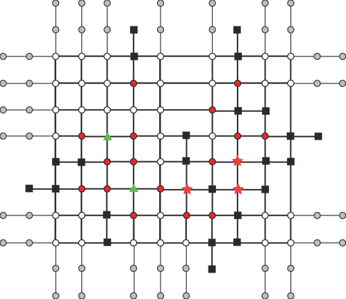
Figure 11: The simplified extended T-mesh $\overline{\mathsf{T}}_{ext}$ for the extended T-mesh in Figure 4.

Lemma 8.3.

The dimension of the null space of $\mathbf{M}$ is the same as that for $\overline{\mathbf{M}}$.

Proof.

The vertex cofactors which correspond to the removed corner vertices can be uniquely determined by applying (15) to the four horizontal removed segments or by applying (16) to the four vertical removed segments. To establish the result we need to show that the constraints corresponding to the four vertical removed segments can be derived from the constraints corresponding to the four horizontal removed segments. We have that

$$0 =\sum_{m=0}^{k}\left[\sum_{\ell=0}^{l}d_{i_{m},j_{\ell}}(\eta-\eta_{j_{\ell}})^{3}\right](\xi-\xi_{i_{m}})^{3}$$ (18)

$$=\sum_{\ell=0}^{l}\left[\sum_{m=0}^{k}d_{i_{m},j_{\ell}}(\xi-\xi_{i_{m}})^{3}\right](\eta-\eta_{j_{\ell}})^{3}$$ (19)

$$=\sum_{\ell=0,1,l-1,l}\left[\sum_{m=0}^{k}d_{i_{m},j_{\ell}}(\xi-\xi_{i_{m}})^{3}\right](\eta-\eta_{j_{\ell}})^{3}.$$ (20)

Equation (18) involves the sum of all edge conformality conditions for the horizonal edge segments. Equation (20) holds because the linear systems for the other vertical segments are satisfied. Since $(\eta-\eta_{j_{\ell}})^{3}$, $\ell=0,1,l-1,l$, form a basis for a linear space of polynomials with degree less than four, $\sum_{m=0}^{k}d_{i_{m},j_{\ell}}(\xi-\xi_{i_{m}})^{3}=0$, for $m=0,\ldots,k$. In other words, the constraints for the four vertical removed segments can be derived from the other constraints. ∎

Remark 8.4.

There are many possible simplification techniques which could have been used. This simplication technique was chosen because it leaves the null space of $\mathbf{M}$ undisturbed and each resulting segment in $\overline{\mathbf{M}}$ contains exaclty four extended vertices.

Theorem 8.5.

If $\overline{\mathbf{M}}$ has full column rank, then the dimension of $\mathcal{S}_{ext}$ is

$$\begin{array}[]{r@{\;}l}\dim\mathcal{S}_{ext}=n^{a}+n^{+}+n^{-}\end{array}$$ (21)

where $n^{a}$ is the number of active vertices in $\mathsf{T}$ and $n^{+}$ and $n^{-}$ are the number of crossing and overlap vertices, respectively, in $\mathsf{T}_{ext}$.

Proof.

Since there are $\overline{n}^{ext}$ and $\overline{n}^{G}$ vertices and segments, respectively, in $\overline{\mathsf{T}}_{ext}$, $\overline{\mathbf{M}}$ is a $4\overline{n}^{G}\times\overline{n}^{ext}$ matrix. Since $\overline{\mathbf{M}}$ has full column rank the dimension of $\mathcal{S}_{ext}$ is $\overline{n}^{ext}-4\overline{n}^{G}$. As every segment in $\overline{\mathsf{T}}_{ext}$ has exactly four extended vertices and these four extended vertices are not extended vertices for any other segment, the number of extended vertices in $\overline{\mathsf{T}}_{ext}$ is $4\overline{n}^{G}$. Thus,

$$\begin{array}[]{r@{\;}l}\dim\mathcal{S}_{ext}=\overline{n}^{ext}-4\overline{n}^{G}=n^{a}+n^{+}+n^{-}.\end{array}$$ (22)

∎

8.3 Rank of the constraint matrix $\overline{\mathbf{M}}$

Since every extended vertex in $\overline{\mathsf{T}}_{ext}$ is an extended vertex in exactly one segment, the matrix $\overline{\mathbf{M}}$ has more columns than rows, i.e., $\overline{n}^{ext}>4\overline{n}^{G}$. After arranging the order of edge conformality conditions and the order of vertex cofactors, an appropriate partition of the linear system of constraints, $\overline{\mathbf{M}}\,\,\overline{\mathbf{D}}=\mathbf{0}$, is

$$\left[\begin{array}[]{c|c}\overline{\mathbf{M}}_{1}&\overline{\mathbf{M}}_{2}\end{array}\right]\left[\begin{array}[]{c}\overline{\mathbf{D}}_{1}\vspace{2pt}\\ \hline\cr\vspace{-10pt}\hfil\\ \overline{\mathbf{D}}_{2}\end{array}\right]=\mathbf{0}$$ (23)

where $\overline{\mathbf{M}}_{1}$ is a $4\overline{n}^{G}\times 4\overline{n}^{G}$ matrix and $\overline{\mathbf{M}}_{1}$ is a $4\overline{n}^{G}\times(\overline{n}^{ext}-4\overline{n}^{G})$ matrix, $\overline{\mathbf{D}}_{1}$ is a vector of the first $4\overline{n}^{G}$ vertex cofactors, and $\overline{\mathbf{D}}_{2}$ is a vector of the remaining vertex cofactors.

Definition 8.6.

A simplified extended T-mesh is called diagonalizable if we can arrange all the segments $G_{i},i=1,\dots,\overline{n}^{G}$ such that the number of vertices on segment $G_{j}$ but not on segment $G_{i},i<j$ is at least 4.

Lemma 8.7.

If a simplified extended T-mesh is diagonalizable, then the matrix $\overline{\mathbf{M}}$ has full column rank.

Proof.

Since the simplified extended T-mesh is diagonalizable, the segments can be ordered as described in Definition 8.6. Given this ordering of segments, for $i=1,\ldots,\overline{n}^{G}$, we place the edge conformality conditions corresponding to segment $G_{i}$ in rows $4(\overline{n}^{G}-i)+1$ through $4(\overline{n}^{G}-i)+4$ of $\overline{\mathbf{M}}$, and place the first four vertex cofactors which appear in $G_{i}$ but not in $G_{j},j<i$ in columns $4(\overline{n}^{G}-i)+1$ through $4(\overline{n}^{G}-i)+4$ of $\overline{\mathbf{D}}_{1}$. Then the matrix $\overline{\mathbf{M}}_{1}$ is in upper block triangular form and according to Lemma 8.1 each diagonal block $4\times 4$ matrix is full rank, thus matrix $\overline{\mathbf{M}}_{1}$ is obviously of full rank. ∎

Lemma 8.8.

$\overline{\mathsf{T}}_{ext}$ is diagonalizable if and only if for any set of segments there exists at least one segment in the set that has at least four vertices which are not in the other segments in the set.

Proof.

Assume the T-mesh is diagonalizable but there exists a set of segments $\{G_{i_{j}},j=1,\dots,s\}$ such that any segment in the set has at most three vertices which are not on the other segments in the set. Without loss of generality, assume the diagonalizable segment ordering for $\overline{\mathsf{T}}_{ext}$ is $G_{i},i=1,\dots,\overline{n}^{G}$. Let $k$ be the maximal index for all $i_{j},j=1,\dots,s$ and consider the set $\{G_{i},i=1,\dots,k\}$. Since $G_{k}$ has at most three vertices which are not in the segments $G_{i_{j}},j=1,\dots,s$, there exists an index $i,i<k$ such that the number of vertices on segment $G_{k}$ but not on segment $G_{i}$ is at most three. This violates the assumption that $\overline{\mathsf{T}}_{ext}$ is diagonalizable.

Suppose for any set of segments in $\overline{\mathsf{T}}_{ext}$ there exists at least one segment which has at least four vertices which are not on the other segments in the set. For the set containing every segment, according to the assumption, there exists one segment, $G_{\overline{n}^{G}}$, which has at least four vertices which are not on the other segments. Now, removing $G_{\overline{n}^{G}}$ from the set, we have that in the set of remaining segments there exists one segment, $G_{\overline{n}^{G}-1}$, which has at least four vertices which are not on the other segments. Continuing this process, we can arrange all the segments $G_{i},i=1,2,\dots,\overline{n}^{G}$ such that the number of vertices on segment $G_{j}$ but not on segment $G_{i},i<j$ is at least 4. Thus $\overline{\mathsf{T}}_{ext}$ is diagonalizable. ∎

Theorem 8.9.

For an analysis-suitable T-mesh, matrix $\overline{\mathbf{M}}$ has full column rank.

Proof.

For an analysis-suitable T-mesh we will prove that the corresponding simplified extended T-mesh is diagonalizable. Otherwise, according to Lemma 8.8, there exists a set of segments such that each segment in the set has at most three vertices which are not on the other segments in the set. It is evident that the set must contain horizonal segments. Otherwise, any vertical segment violates the assumption because it must have at least four vertices which are not in the other segments in the set. Let $G_{i}$ be the bottommost horizonal segment in the set (if there is more than one such segment choose one of them). Since $G_{i}$ has at most three vertices which are not on the other segments in the set, one of the four extended vertices of $G_{i}$ must lie on a vertical segment, $G_{j}$. Now, referring to Figure 12, since the T-mesh is analysis-suitable, $G_{j}$ must have two anchor vertices whose vertical index coordinate is less than $a$. Otherwise, the T-mesh is not analysis-suitable due to intersecting T-juction extensions. Additionally, $G_{j}$ must have two extended vertices whose vertical index coordinate is less than $a$. Thus, there are four vertices in $G_{j}$ which do not belong to any other segment in the set which contradicts the assumption. ∎

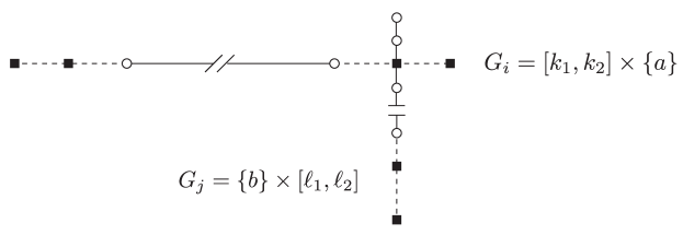
Figure 12: A schematic for Theorem 8.9.

9 Conclusion

We have established several important properties of analysis-suitable T-splines. We developed a characterization of ASTS spaces and proved that the space of bicubic polynomials, defined over the extended T-mesh of an ASTS, is contained in the corresponding ASTS space. We then proved the conditions under which two ASTS spaces are nested. This provides the theoretical foundation for the analysis-suitable local refinement algorithm in [3]. Using the characterization of ASTS we then proved several basic approximation results. Additionally, we developed the theory of perturbed ASTS and a simple mesh-based dimension formula which is written in terms of the vertices in the extended T-mesh of a T-spline. Both of these developments were critical for the proofs in this paper and may have important applications in other contexts. While the developments in this paper are restricted to bicubic surfaces the extension to arbitrary degree should be straightforward.

Appendix A Notational conventions

In Tables 2 and 3 the notational conventions used throughout the text are listed as well as the section where they are defined.

Table 2: Notational conventions used throughout the text and where they are defined.

Symbols	Description	Section
$\mathsf{T}$	A T-mesh	2.1
$\mathsf{V}$	All vertices in a T-mesh	2.1
$\mathsf{E}$	All edges in a T-mesh	2.1
$\mathsf{S}$	The skeleton of a T-mesh	2.1
$h\mathsf{S}$ $(v\mathsf{S})$	The horizontal (vertical) skeleton of a T-mesh	2.1
$Q$	An element of a T-mesh	2.1
$\mathsf{G}$	All segments in a T-mesh	2.4
$n^{G}$	The number of segments in a T-mesh	2.4
$h\mathsf{G}$ ($v\mathsf{G}$)	All horizontal (vertical) segments in a T-mesh	2.4
$h\mathsf{G}(a)$ $(v\mathsf{G}(a))$	The horizontal (vertical) segments at vertical (horizontal) index $a$	2.4
$\mathsf{R}$	The index domain of a T-mesh	2.1
$\mathsf{AR}$	The active region of an index domain	2.1
$\mathsf{FR}$	The frame region of an index domain	2.1
$\mathsf{T}_{ext}$	An extended T-mesh	2.5
$ext^{f}(\mathsf{T})$	All face extensions in $\mathsf{T}$	2.5
$ext^{f}(T)$	The face extension of T-junction $T$	2.5
$ext^{e}(\mathsf{T})$	All edge extensions in $\mathsf{T}$	2.5
$ext^{e}(T)$	The edge extension of T-junction $T$	2.5
$ext(\mathsf{T})$	All extensions in $\mathsf{T}$	2.5
$ext(T)$	The extension of T-junction $T$	2.5
$hext^{f}(\mathsf{T})$ $vext^{f}{\mathsf{T}}$	All horizontal (vertical) faces extensions in a T-mesh	2.5
$\mathsf{CV}$	All crossing vertices in $\mathsf{T}_{ext}$	2.5
$n^{+}$	The number of crossing vertices in $\mathsf{T}_{ext}$	2.5
$\mathsf{OV}$	All overlap vertices in $\mathsf{T}_{ext}$	2.5
$n^{-}$	The number of overlap vertices in $\mathsf{T}_{ext}$	2.5
$\mathsf{EV}$	All extended vertices in $\mathsf{T}_{ext}$	2.5
$n^{*}$	The number of overlap vertices in $\mathsf{T}_{ext}$	2.5
$n^{ext}$	The number of vertices in $\mathsf{T}_{ext}$	2.5

Table 3: Notational conventions used throughout the text and where they are defined.

Symbols	Description	Section
$\mathsf{A}(\mathsf{T})$	All anchors in a T-mesh	2.3
$n^{A}$	The number of anchors in a T-mesh	2.3
$\mathsf{J}$	The set of T-junctions in a T-mesh	2.3
$hv(A)$ ($vv(A)$)	The horizontal (vertical) local index vector for $N_{A}(\xi,\eta)$	3
$\Xi_{A}$ ($\Pi_{A}$)	The horizontal (vertical) local knot vector for $N_{A}(\xi,\eta)$	3
$\tilde{\Omega}$	The full parametric domain of $\mathsf{T}$	3
$\tilde{Q}$	A T-spline element in the full parametric domain	3
$\hat{\Omega}$	The reduced parametric domain of $\mathsf{T}$	3
$\hat{Q}$	A T-spline element in the reduced parametric domain	3
$\Omega_{\hat{Q}}$	The extended support of $\hat{Q}$	7
$R(\Omega_{\hat{Q}})$	The smallest rectangle containg $\Omega_{hat{Q}}$	7
$N_{A}(\xi,\eta)$	The T-spline blending function for anchor $A$	3
$Q_{A}$	The support of $N_{A}$	7
$\lambda_{A}$	The dual basis function associated with $N_{A}$	3
$\mathcal{T}$	A T-spline space	3
$\mathcal{S}_{ext}$	A homogeneous extended spline space	6
$\mathcal{T}_{ext}$	An extended spline space	6
$\Xi[\boldsymbol{\delta}]$($\Pi[\boldsymbol{\delta}]$)	A horizontal (vertical) perturbed global knot vector	5
$\imath=\imath(i,g)$ ($\jmath=\imath(j,g)$)	the index of the $g^{th}$ segment in $h\mathsf{G}(\{i\})$ ($v\mathsf{G}(\{j\})$)	5
$\pi$	the map from perturbed index $\imath(i,g)$ to index $i$	5
$\mathsf{T}(\boldsymbol{\delta})$	A perturbed T-mesh	5
$\mathcal{T}(\boldsymbol{\delta})$	A perturbed T-spline space	5
$\mathsf{T}(\boldsymbol{\delta},\mathsf{T}^{i})$	A perturbed T-mesh generated from $\mathsf{T}^{i}(\boldsymbol{\delta})$	5

References

- [1] T. W. Sederberg, J. Zheng, A. Bakenov, A. Nasri, T-splines and T-NURCCs, ACM Trans. Graph. 22 (2003) 477–484.
- [2] T. W. Sederberg, D. L. Cardon, G. T. Finnigan, N. S. North, J. Zheng, T. Lyche, T-spline simplification and local refinement, ACM Trans. Graph. 23 (2004) 276–283.
- [3] M. A. Scott, X. Li, T. W. Sederberg, T. J. R. Hughes, Local refinement of analysis-suitable T-splines, Computer Methods in Applied Mechanics and Engineering 213 (2012) 206 – 222.
- [4] H. Ipson, T-spline merging, Master’s thesis, Brigham Young University (2005).
- [5] T. W. Sederberg, G. T. Finnigan, X. Li, H. Lin, Watertight trimmed NURBS, ACM Trans. Graph. 27 (2008) 1–79.
- [6] Y. Bazilevs, V. M. Calo, J. A. Cottrell, J. A. Evans, T. J. R. Hughes, S. Lipton, M. A. Scott, T. W. Sederberg, Isogeometric analysis using T-splines, Computer Methods in Applied Mechanics and Engineering 199 (5-8) (2010) 229–263.
- [7] M. A. Scott, M. J. Borden, C. V. Verhoosel, T. W. Sederberg, T. J. R. Hughes, Isogeometric Finite Element Data Structures based on Bézier Extraction of T-splines, International Journal for Numerical Methods in Engineering, 88 (2011) 126 – 156.
- [8] C. V. Verhoosel, M. A. Scott, T. J. R. Hughes, de Borst, R., An isogeometric analysis approach to gradient damage models, International Journal for Numerical Methods in Engineering, 86 (2011) 115–134.
- [9] C. V. Verhoosel, M. A. Scott, R. de Borst, T. J. R. Hughes, An isogeometric approach to cohesive zone modeling, International Journal for Numerical Methods in Engineering, 87 (2011) 336 – 360.
- [10] M. J. Borden, M. A. Scott, C. V. Verhoosel, C. M. Landis, T. J. R. Hughes, A phase-field description of dynamic brittle fracture, Computer Methods in Applied Mechanics and Engineering 217 (2012) 77 – 95.
- [11] D. J. Benson, Y. Bazilevs, E. De Luycker, M. C. Hsu, M. A. Scott, T. J. R. Hughes, T. Belytschko, A generalized finite element formulation for arbitrary basis functions: From isogeometric analysis to XFEM, International Journal for Numerical Methods in Engineering 83 (2010) 765–785.
- [12] D. Schillinger, L. Dedé, M. A. Scott, J. A. Evans, M. J. Borden, E. Rank, T. J. R. Hughes, An isogeometric design-through-analysis methodology based on adaptive hierarchical refinement of NURBS, immersed boundary methods, and T-spline CAD surfaces, Computer Methods in Applied Mechanics and Engineering accepted for publication.
- [13] M. A. Scott, R. N. Simpson, J. A. Evans, S. Lipton, S. P. A. Bordas, T. J. R. Hughes, T. W. Sederberg, Isogeometric boundary element analysis using unstructured T-splines, Computer Methods in Applied Mechanics and Engineering submitted.
- [14] T. J. R. Hughes, J. A. Cottrell, Y. Bazilevs, Isogeometric analysis: CAD, finite elements, NURBS, exact geometry, and mesh refinement, Computer Methods in Applied Mechanics and Engineering 194 (2005) 4135–4195.
- [15] J. A. Cottrell, T. J. R. Hughes, Y. Bazilevs, Isogeometric analysis: Toward Integration of CAD and FEA, Wiley, Chichester, 2009.
- [16] J. A. Cottrell, A. Reali, Y. Bazilevs, T. J. R. Hughes, Isogeometric analysis of structural vibrations, Computer Methods in Applied Mechanics and Engineering 195 (2006) 5257–5296.
- [17] J. A. Evans, Y. Bazilevs, I. Babuška, T. J. R. Hughes, n-widths, sup-infs, and optimality ratios for the k-version of the isogeometric finite element method, Computer Methods in Applied Mechanics and Engineering 198 (21-26) (2009) 1726–1741.
- [18] S. Lipton, J. A. Evans, Y. Bazilevs, T. Elguedj, T. J. R. Hughes, Robustness of isogeometric structural discretizations under severe mesh distortion, Computer Methods in Applied Mechanics and Engineering 199 (5-8) (2010) 357–373.
- [19] X. Li, J. Zheng, T. W. Sederberg, T. J. R. Hughes, M. A. Scott, On linear independence of T-spline blending functions, Computer Aided Geometric Design 29 (2012) 63 – 76.
- [20] L. Beirão da Veiga, A. Buffa, D. Cho, G. Sangalli, Analysis-suitable t-splines are dual-compatible, Computer Methods in Applied Mechanics and Engineering.
- [21] L. B. da Veiga, A. Buffa, G. Sangalli, R. Vázquez, Analysis-suitable T-splines of arbitrary degree: definition and properties, submitted.
- [22] Y. Bazilevs, L. Beirao de Veiga, J. Cottrell, T. J. R. Hughes, G. Sangalli, Isogeometric analysis: approximation, stability and error estimates for -refined meshes, Mathematical Models and Methods in Applied Sciences 16 (2006) 1031–1090.
- [23] T. J. R. Hughes, The Finite Element Method: Linear Static and Dynamic Finite Element Analysis, Dover Publications, Mineola, NY, 2000.
- [24] L. Schumaker, Spline functions: basic theory, Krieger, 1993.
- [25] R. Wang, Multivariate spline functions and their applications, Kluwer Academic Publishers, 2001.