Renormalization of two-body interactions due to higher-body interactions of lattice bosons

Abstract

We calculate thermodynamic properties of soft-core lattice bosons with on-site $n$-body interactions using up to twelfth and tenth order strong coupling expansion in one and two dimensional cubic lattices at zero temperature. Using linked cluster techniques, we show that it is possible to exactly renormalize the two-body interactions for quasiparticle excitations and ground-state energy by resumming the three and four body terms in the system, which suggests that all higher-body on-site interactions may be exactly and perturbatively resummed into the two-body terms for similar system observables. The renormalization procedure that we develop is applicable to a broad range of systems analyzable by linked cluster expansions, ranging from perturbative quantum chromodynamics to spin models, giving either an exact or approximate resummation depending on the specific system and properties. Universality at various three-body interaction strengths for the two dimensional boson Hubbard model is checked numerically.

I Introduction

The first calculation of the effect of three-body interactions in lattice bosons Murphy for liquid He⁴ and solid He revealed its negligible effect on its ground state energy. However, it was recently suggested Buechler that, firstly, three-body interactions in cold polar molecules could be naturally modelled by Hubbard Hamiltonians with nearest-neighbour three-body terms and, secondly, there might arise new exotic phases in experimental setups of such degenerate quantum molecular gases. Shortly thereafter, a decoupling mean-field (MF) approximation was used to investigate the critical properties of a boson Hubbard model with on-site three-body interactions Zhang . That such on-site terms could effectively arise in two-body collisions of atoms confined to optical lattices was only subsequently justified Johnson . Indeed such a multi-body interaction Hamiltonian, of the form Eq. (1) that we study, was observed through quantum phase revivals in a system of ultracold ${}^{87}\textrm{Rb}$ atoms with virtual transitions from the lowest vibrational state to higher energy bands Will .
We employ a strong coupling expansion $-$ which suffers from no finite size effects as it operates directly in the thermodynamic limit $-$ of the on-site three-body interacting boson Hubbard model, in addition to checking the universality hypothesis at $XY$ critical points for various three-body strengths. A procedure for incorporating higher body interactions by renormalizing the two-body problem will also be described herein.
Consider a system of two-body and higher-body interacting bosons on the one dimensional chain and two dimensional square lattices described by the Hamiltonian

$$H = -t\sum_{<i,j>}(b_{i}^{\dagger}b_{j}^{\phantom{\dagger}}+\textrm{h.c})+\frac{U}{2}\sum_{i}\hat{n_{i}}(\hat{n_{i}}-1)$$ (1)

$$+\sum_{k=3}\frac{U_{k}}{k!}\sum_{i}\prod_{l=0}^{k-1}(\hat{n_{i}}-l)-\mu\sum_{i}\hat{n_{i}}.$$

where the $b_{i}^{\dagger}$ and $b^{\phantom{\dagger}}_{i}$ are bosonic creation and annihilation operators, $\hat{n_{i}}=b_{i}^{\dagger}b_{i}^{\phantom{\dagger}}$ is the number operator, the hopping-terms $t$ are between nearest neighbors, and the system consists of a single species of soft-core bosons. The local energy term $U$ contributes to a repulsive on-site interaction between bosons, $U_{k}>0$ is the strength of $k$-body on-site interaction terms and $\mu$ is the chemical potential. The onsite term $U$ will be the energy scale of choice in this letter.
The Hamiltonian in Eq. (1), when represented in the form $\mathcal{H}=\mathcal{H}_{0}-\lambda\mathcal{H}_{1}$ with $\mathcal{H}_{1}$ being the hopping terms of strength $\lambda=t/U$ and $\mathcal{H}_{0}$ being the rest of Eq. (1), is amenable to linked cluster expansions Singh ; Elstner in the parameter $\lambda$. Evaluation of physical properties e.g. energy are performed via Rayleigh-Schrödinger perturbation theory Baym and the linked cluster expansion. Excited states can be obtained using a similar procedure through Gelfand’s similarity transformation Singh .

II Critical properties

In this section we focus on the critical properties of the transition between the ground state Mott insulator and the superfluid phase in the Bose-Hubbard model. The quantum phase transition at the tip of the insulating lobe will be a special point of concern because the system’s universality with the XY model may be investigated at this multicritical point Fisher ; Freericks .

II.1 One dimensional chain lattice

Consider first the $\rho=1$ Mott insulating lobe in the one dimensional chain. For a twelfth order bond-expansion, there are 13 distinct topological graphs (clusters) that can be embedded on the infinite chain: approximately 2.5 million states contribute to the full Hilbert space with a maximum of 13 states in the lowest degenerate manifold. From MF calculations Zhang ; Shou , it was predicted that the first Mott lobe should not change in structure; this was later systematically corrected by density matrix renormalization group (DMRG) calculations Valencia ; MSingh and exact diagonalization Sowinski . Using Gelfand’s similarity transformations to construct the particle and hole excitations, we identify the disappearance of the excitation gap as defining the second-order transition contours of the lobe: we have thus evaluated the series for the gap up to twelfth order; moreover we emphasize that because we work in the thermodynamic limit, there are no finite size effects in the sense that each of the coefficients in the series are exact to any given perturbative order. To illustrate, for $r_{3}\equiv\frac{U_{3}}{U}=1$, the first eight terms in the Mott gap, $\delta_{1}(\lambda,{\bf k}=0)$, are given by

$$\delta_{1}(\lambda,{\bf k}=0)=1-6\lambda+6\lambda^{2}+\frac{20}{3}\lambda^{3}-\frac{46}{27}\lambda^{4}+\frac{30751}{243}\lambda^{5}-\frac{185083}{324}\lambda^{6}+\frac{464023295}{157464}\lambda^{7}-\frac{68401014192209}{3769688160}\lambda^{8},$$ (2)

where ${\bf k}$ is the lattice momentum. In Fig. 1 we show particle and hole contours obtained by multiple precision Padé approximation of twelfth order series and compared to a previously published Valencia DMRG solution for $r_{3}=7$. The location of the critical point (Kosterlitz-Thouless transition) shifts upwards and rightwards in the phase diagram indicating an increase in the size of the first lobe and a partial restoration of particle-hole symmetry as the semi-hardcore condition ($r_{3}=\infty$) is reached. We have verified this tendency with $r_{3}=0,1,7,100$. For the hardcore condition, the critical $\mu/U$ ($U$ now being the nearest neighbour repulsion) equals exactly 1 Yang , with the particle-hole symmetry completely restored.

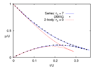
Figure 1: First Mott lobe in the ground state phase diagram of the one dimensional boson Hubbard model with various $r_{3}\equiv\frac{U_{3}}{U}$ ratios; the last Padé approximant [6/6] or [5/5] of the twelfth order gap series for $r_{3}=7$ is compared with a DMRG solution Valencia . [m/n] denotes an $m^{\textrm{th}}$ order numerator and an $n^{\textrm{th}}$ order denominator. The Kosterlitz-Thouless point shifts upwards and rightwards as $r_{3}$ is increased.

We note that in an $n$-th order bond expansion for the linear chain, we need calculate the $n$-th order particle and hole contributions only up to graphs with $n-1$ bonds: the effective Hamiltonian for the last cluster may be calculated with very little effort because, within the degenerate subspace of this graph, the only contributing process will be the one which transfers the excitation from one end of the chain to the other. We find that these matrix elements are simply given by the negative of the Schroeder numbers $S=\{1,2,6,22,90\cdots\}$ with the generating function Sloane

$$G(x)=\frac{1-x-\sqrt{1-6x+x^{2}}}{2x}.$$

That is, for a cluster with $n$-bonds the $n^{\textrm{th}}$ order effective Hamiltonian has its non-zero elements given by $H(0,n)=-S_{n-1}$, for $l\geq 2$. This is independent of $r_{3}$ and the type of excitation.

II.2 Two dimensional square lattice

In two dimensions there are 680 topologically distinct clusters contributing at tenth order for a bond-expansion. Here the Mott gap closes as $\delta\propto(t_{c}-t)^{z\nu}$ Fisher for $t-t_{c}\ll 1$, assuming the universality of the $XY$ model: $t_{c}$ is the value of the hopping element at the multicritical point where particle-hole symmetry is restored (here $z=1$), $z$ and $\nu$ are the dynamical and coherence length critical exponents respectively. To investigate the effect of three-body terms in 2D, we have calculated tenth order series for the $\rho=1$ Mott gaps for $r_{3}=1,10,100$. From these series’, $t_{c}$ and $z\nu$ may be extracted by proceeding, mutatis mutandis, as outlined in previous scaling analysis Elstner ; Varma : (a) by linearly extrapolating the roots of the truncated gap series’ from, say, fourth to tenth order and (b) by Padé approximating the gap series’ to mimic the expected $\delta$ behaviour mentioned above. The results of the higher approximants ([4/4], [4/5], [4/6], [5/4], [5/5]) and linear extrapolation are tabulated in Table 1 for four $r_{3}$ values: it must be noted that large $r_{3}$ values may be attained, as suggested by Johnson et. al., using Feshbach resonances and tuning the lattice potential. As can be noted from the table that the change in $t_{c}$ upon increasing $r_{3}$, and hence the structure of the first lobe, is not as substantial for the square lattice as was seen for the one dimensional case. From the $\nu$ values for the four three-body interaction strengths, we see that universality does indeed seem to hold at the $XY$ point. The corresponding classical critical coefficient for the three dimensional $XY$ model is $\nu=0.67155\pm 0.00027$ Campostrini .

Table 1: Critical points and exponents for the two dimensional square lattice boson Hubbard model at various three-body interactions $r_{3}$ using roots extrapolation (E) and Padé approximations (P). See text and Refs. 7 and 17 for the exact procedure. At the critical point $t=t_{c}$, $z=1$ Fisher .

$r_{3}$	$t_{c}^{\textrm{E}}$($10^{-4}$)	$t_{c}^{\textrm{P}}$($10^{-4}$)	$\nu$($10^{-3}$)
0	597.4 $\pm$ 0.4	599	690
1	603.8 $\pm$ 0.8	604.69 $\pm$ 0.06	692.3 $\pm$ 0.6
10	616.7 $\pm$ 0.8	617.39 $\pm$ 0.05	695.4 $\pm$ 0.4
100	621.4 $\pm$ 0.8	621.98 $\pm$ 0.06	696.5 $\pm$ 0.5

III Renormalization procedure

In general, to incorporate a second variable like $U_{3}$ into a Hamiltonian within linked cluster expansions requires a double-expansion: the first in $t/U$, the second in $U_{3}/U$. For example, the double-expansion of a quantity $P$ in perturbing variables $\lambda$ and $r$ to order $M$ and $N$ respectively may be symbolically written as

$$P=\sum_{i}^{M}c_{1i}^{(N)}\lambda^{i},$$

$$c_{1i}^{(N)}=\sum_{j}^{N}c_{2j}r^{j}.$$ (3)

Now $M$ and $N$ are finite integers but can one do better? The prescription we adopt is to resum the second series and evaluate $\lim_{N\to\infty}c_{1i}^{(N)}$ for every $i$, keeping $M$ finite, and is implemented as follows: we first calculate the series coefficients for a given observable (like in Eq. 2) for a finite number of $r_{3}$ values. And because the coefficients are always rational numbers $-$ by virtue of the perturbation theory $-$ it only remains to find a rational function approximation to the obtained coefficients. The latter step may be easily implemented with Thiele’s algorithm for continued fraction representation Stoer .

III.1 Thiele’s algorithm

Thiele’s algorithm is used to interpolate a given set of support points $(x_{i},f_{i})$ by a rational function of the form

$$\mathbf{\phi}^{(M,N)}(x)=\frac{P^{(M)}(x)}{Q^{(N)}(x)}=\frac{a_{0}+a_{1}x+\cdots+a_{M}x^{M}}{b_{0}+b_{1}x+\cdots+b_{N}x^{N}},$$ (4)

for integer coefficients $a_{i},b_{i}$ and some order of the polynomials $M,N$. As with the construction of Padé approximants, the maximal degree of the numerator and denominator in Thiele’s rational function approximation are determined by the number of data points available. We closely follow the discussion in Ref. 19 in this subsection.
Rational expressions are constructed along the main diagonal of the $(M,N)$-plane in Thiele’s algorithm. The support points $(x_{i},f_{i})$ are used to generate inverse differences $\phi$ depicted notationally in Table 2. The inverse differences and the algorithm are defined by the following recursion relation and identity Stoer

$$\phi(x_{i},x_{j}) = \frac{x_{i}-x_{j}}{f_{i}-f_{j}},$$

$$\phi(x_{i},\ldots,x_{l},x_{m},x_{n}) = \frac{x_{m}-x_{n}}{\phi(x_{i},\ldots,x_{l},x_{m})-\phi(x_{i},\ldots,x_{l},x_{n})},$$

$$\phi^{(n,n)}(x) = f_{0}+\begin{array}[]{@{}c@{}}\lx@intercol\hfil x-x_{0}\hfil\lx@intercol\vrule\lx@intercol\\ \hline\cr\vrule\lx@intercol\hfil\phi(x_{0},x_{1})\hfil\lx@intercol\end{array}$$ (7)

$$+ \begin{array}[]{@{}c@{}}\lx@intercol\hfil x-x_{1}\hfil\lx@intercol\vrule\lx@intercol\\ \hline\cr\vrule\lx@intercol\hfil\phi(x_{0},x_{1},x_{2})\hfil\lx@intercol\end{array}+\ldots$$ (10)

$$+ \cfrac{x-x_{2n-1}}{\phi(x_{0},x_{1},\ldots,2n)}.$$ (11)

The last three lines in (III.1) gives the continued fraction expansion, in Pringsheim’s notation, for the Thiele’s rational approximation of the $2n+1$ data points.

Table 2: Generic flow of the Thiele’s algorithm in construction of inverse differences from the input data set.

$x_{i}$	$f_{i}$	Inverse differences
$x_{0}$	$f_{0}$
$x_{1}$	$f_{1}$	$\phi(x_{0},x_{1})$
$x_{2}$	$f_{2}$	$\phi(x_{0},x_{2})$      $\phi(x_{0},x_{1},x_{2})$
$x_{3}$	$f_{3}$	$\phi(x_{0},x_{2})$      $\phi(x_{0},x_{1},x_{2})$      $\phi(x_{0},x_{1},x_{2},x_{3})$
$\vdots$	$\vdots$	$\vdots$

Table 3: Resummed series coefficients for the particle and hole contours in the one dimensional chain and two dimensional square lattice. Coefficients of lower order that are not listed are independent of $r_{3}$.

	Lattice
Coefficient	1D	2D
$c_{4}^{-}$	$\cfrac{60-4r_{3}}{3+r_{3}}$	$-8\cfrac{231+71r_{3}}{3+r_{3}}$
$c_{2}^{+}$	$2\cfrac{1+2r_{3}}{2+r_{3}}$	$-4\cfrac{7+2r_{3}}{2+r_{3}}$
$c_{3}^{+}$	$12\cfrac{2+2r_{3}+r_{3}^{2}}{(2+r_{3})^{2}}$	$-24\cfrac{20+18r_{3}+3r_{3}^{2}}{(2+r_{3})^{2}}$
$c_{4}^{+}$	$-2\cfrac{339+1631r_{3}+2818r_{3}^{2}+2088r_{3}^{3}+676r_{3}^{4}+80r_{3}^{5}}{(2+r_{3})^{3}(3+r_{3})(5+4r_{3})}$	$-4\cfrac{28497+71317r_{3}+70166r_{3}^{2}+33672r_{3}^{3}+7772r_{3}^{4}+688r_{3}^{5}}{(2+r_{3})^{3}(3+r_{3})(5+4r_{3})}$

In the event that one or more of the inverse differences in Table 2 are equal, then the continued fraction expansion must terminate at this column lest the succeeding inverse differences become undefined; this abrupt termination usually indicates that the obtained approximation is in fact an exact functional representation of the input data.
To summarize, the functional dependence of a coefficient at a given order on $r_{3}$ is to be captured by a rational approximation. For example, a single-expansion coefficient $c_{1i}$, for a given $i$, for some 24 values of $r_{3}$ from $0\rightarrow 100$ were evaluated. Thiele’s algorithm to find an approximating rational function $f_{i}(r_{3})=c_{1i}(r_{3})$ would generally require as many steps as there are points (here 24) to terminate and find the best fit; however, we find that in each of the evaluated coefficients, the algorithm stops exactly after a few steps because the continued fraction expansions stop. This ensures the exactness of the obtained $f_{i}(r_{3})$. With this, the $c_{1}$’s in Eq. 3 get fully renormalized by the resummed $c_{2}$’s.

III.2 Three body interactions

The procedure in Sec. III.1 can now be applied to renormalizing the series coefficients of the particle and hole contours in the two-body interacting one dimensional chain and two dimensional square lattice with respect to the three body terms. Let the particle and hole contours, for any $r_{3}$, be represented as

$$\pm\mu_{\pm}^{c}(r_{3})=\sum_{i=0}c_{i}^{\pm}(r_{3})\lambda^{i}.$$ (12)

The signs ($\pm$) refer to the particle and the hole contours respectively. For illustrating our method, we sketch in Fig. 2 the [1/1] rational function approximation to $c_{4}^{-}(r_{3})$ in the one dimensional chain obtained from the 24 different values of $r_{3}$. The same analyses were performed for the particle coefficients as well and similar conclusions hold; the resummed coefficients are listed in Table 3 up to fourth order. For example, in the 1D case, $c_{4}^{-}(r_{3}=1)+c_{4}^{+}(r_{3}=1)=-\frac{46}{27}$, the fourth coefficient in Eq. 2. It is worth noting that even with coefficients for particle-hole series only up to third order, very reasonable estimates (within 10% compared to more accurate results Elstner ) for critical properties can be obtained Freericks . A similar resummation may be readily obtained, exactly and without using the above resummation procedure, for the ground state energy per site $\langle\psi|\mathcal{H}|\psi\rangle$ $-$ where $|\psi\rangle$ is the ground state wavefunction constructed order by order for the first lobe $-$ in the one dimensional chain for an arbitrary $r$ up to fourth order to give

$$E_{0}^{1D}=-4\lambda^{2}+12\frac{1+r_{3}}{3+r_{3}}\lambda^{4}.\\$$ (13)

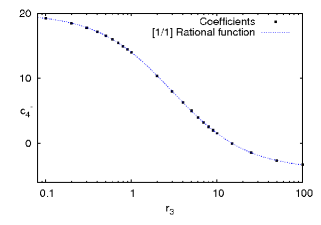
Figure 2: Fourth order coefficient for the hole contour in the one dimensional chain as a function of the three-body interacting strength in a log plot. The coefficient at $r_{3}=0$ passes through the function as well. The [1/1] function for $c_{4}^{-}$ is $\frac{60-4r_{3}}{3+r_{3}}$.

It has been checked that the result (13) is also obtained by employing the renormalization procedure described in Sec. III.1.
We see from Table 3 and Eq. (13) that for certain values of attractive interactions i.e. $r_{3}<0$ there is a perturbative instability of the $\rho=1$ Mott phase coming from the divergence of the denominators. This might signal the disappearance of the first lobe altogether or the appearance of a higher-density and energetically more favourable lobe in that region of phase space: quite naturally, for attractive bosons, higher density Mott phases should stabilize the system and one should expand thermodynamic variables perturbatively about this more favourable phase. Similar conclusions were in fact reached by recent MF and quantum Monte Carlo calculations Naini . In the present work, however, the value of the attractive three-body strength that leads to an instability at a given perturbative order can be readily read off from the resummed coefficients.

III.3 Four body interactions

Using the above procedure for the Hamiltonian with four body interactions, with $r_{4}\equiv\frac{U_{4}}{U}$, we find that the two-body interactions for the ground state energy densities of the linear chain and the square lattice may also be perturbatively renormalized by the four-body terms as given by the following:

$$E_{0}^{\textrm{1D}} = -4\lambda^{2}+4\lambda^{4}+\frac{272}{9}\lambda^{6}+\frac{4(85r_{4}-7602)}{81(r_{4}+6)}\lambda^{8}-\frac{2(252109r_{4}^{3}+2870730r_{4}^{2}+6509628r_{4}-9540936)}{729(r_{4}+6)^{3}}\lambda^{10}+\cdots,$$

$$E_{0}^{\textrm{2D}} = -8\lambda^{2}-24\frac{7r_{4}+27}{r_{4}+3}\lambda^{4}-32\frac{514r_{4}^{4}+6333r_{4}^{3}+28167r_{4}^{2}+53160r_{4}+35217}{(r_{4}+3)^{3}(2r_{4}+3)}\lambda^{6}+\cdots.$$ (14)

Therefore it seems very likely that two-body terms in the Bose-Hubbard model, irrespective of dimension, may be perturbatively renormalized by all higher-body on-site terms for its thermodynamic and excited properties. An interesting question is if such resummability might also exist for dynamical properties and for bosonic models with intersite interactions.

IV Summary

In conclusion, we have presented a way of resumming the effect of a second perturbing variable to infinite order thereby effectively renormalizing the series coefficients of the single variable expansions. The procedure is quite general and may be applied to renormalize the second interaction term in the Hamiltonian in the series expansion representation of any thermodynamic quantity. In the scenario considered, we have found perturbative renormalizations of the two-body interactions due to three and four body terms in calculations of ground state energies and quasiparticle excitations, for the one and two dimensional Bose-Hubbard model. The applicability of the procedure is, of course, not restricted to lattice bosons but can be extended to other systems that are treated using series expansion techniques, ranging from spin models to perturbative quantum chromodynamics where the analytic continuation of strong coupling expansions is still fraught with problems Oitmaa . Additionally, the universality hypothesis of the two dimensional Bose-Hubbard model has been checked for various three body interaction strengths.

V Acknowledgment

One of us (VKV) thanks the Bonn-Cologne Graduate School for support within the Deutsche Forschunggemeinschaft’s Research Funding.

References

- [1] R.D. Murphy and J.A. Baker. Phys. Res. A, 3:1037, 1971.
- [2] H.P. Buechler, A. Micheli, and P. Zoller. Nat. Phys., 3:726, 2007.
- [3] B.L. Chen, X.B. Huang, S.P. Kou, and Y. Zhang. Phys. Rev. A, 78:043603, 2008.
- [4] P.-R. Johnson, E. Tiesinga, J. V. Porto, and C. J. Williams. New Journal of Physics, 11:093022, 2009.
- [5] Sebastian Will, Thorsten Best, Ulrich Schneider, Lucia Hackermuller, Dirk-Soren Luhmann, and Immanuel Bloch. Adv. in Phys., 49:93, 2000.
- [6] M.P. Gelfand and R.R.P. Singh. Adv. in Phys., 49:93, 2000.
- [7] N. Elstner and H. Monien. Phys. Rev. B, 59:12184, 1999.
- [8] Gordon Baym. Lectures on Quantum Mechanics. Lecture Notes and Supplements in Physics. Benjamin/Cummings, England, 1969.
- [9] Matthew P. A. Fisher, Peter B. Weichman, G. Grinstein, and Daniel S. Fisher. Phys. Rev. B, 40:564, 1989.
- [10] J.K. Freericks and H. Monien. Phys. Rev. B, 53:2691, 1996.
- [11] Kezhao Zhou, Zhaoxin Liang, and Zhidong Zhang. Phys. Rev. A, 82:013634, 2010.
- [12] J. Silva-Valencia and A.M.C Souza. Phys. Rev. A, 84:065601, 2011.
- [13] Manpreet Singh, Arya Dhar, Tapan Mishra, R. V. Pai, and B. P. Das. Phys. Rev. A, 85:051604(R), 2012.
- [14] Tomasz Sowiński. Phys. Rev. A, 85:065601, 2012.
- [15] C.N. Yang and C.P. Yang. Phys. Rev., 151:258, 1966.
- [16] The on-line encyclopedia of integer sequences. http://oeis.org/A006318, 2012.
- [17] V.K. Varma and H. Monien. Phys. Rev. B, 84:195131, 2011.
- [18] Massimo Campostrini, Martin Hasenbusch, Andrea Pelissetto, Paolo Rossi, and Ettore Vicari. Phys. Rev. B, 63:214503, 2001.
- [19] J. Stoer and R. Bulirsch. Introduction to Numerical Analysis. Texts in Applied Mathematics. Springer, 3 edition, 2002.
- [20] A. Safavi-Naini, J. von Stecher, B. Capogrosso-Sansone, and Seth T. Rittenhouse. Phys. Rev. Lett., 109:135302, 2012.
- [21] Jaan Oitmaa, Chris Hamer, and Weihong Zheng. Series Expansion Methods for Strongly Interacting Lattice Models. Cambridge University Press, Cambridge, 1 edition, 2006.