Cosmological constraints on spontaneous R-symmetry breaking models

Abstract

We study general constraints on spontaneous R-symmetry breaking models coming from the cosmological effects of the pseudo Nambu-Goldstone bosons, R-axions. They are substantially produced in the early Universe and may cause several cosmological problems. We focus on relatively long-lived R-axions and find that in a wide range of parameter space, models are severely constrained. In particular, R-axions with mass less than 1 MeV are generally ruled out for relatively high reheating temperature, $T_{R}>10$ GeV.

I Introduction

Supersymmetry (SUSY) has been considered to be the strongest candidate of the physics beyond the standard model (BSM). Although the recent data from the Large Hadron Collider (LHC) has not shown any evidence for SUSY but discovered a Standard Model Higgs-like particle with a mass of around 125 GeV LHChiggs , it still remains a strong candidate of BSM because it suggests the gauge coupling unification, it guarantees proton stability sufficiently, and it provides a reasonable dark matter candidate. Moreover, in string theories, which are the most powerful candidates of the quantum theory of gravity, it plays a crucial role for consistency and must be broken at a scale between the electroweak scale and the Planck scale. Therefore, it is important to investigate SUSY-breaking models in the light of LHC data SUSYiloHiggs .

R-symmetry, which is a specific symmetry of supersymmetric models, is a key ingredient for SUSY breaking and its application to model building. Recent drastic progresses on SUSY breaking by exploiting a metastable state (see rev1 ; rev2 ; rev3 for reviews and references therein) gives us a better understanding of the role of the R-symmetry in realistic model building Kitano1 ; Kitano2 ; Intriligator:2007py ; KOO ; Abe:2007ax ; R1 ; R2 ; Kang:2012fn ; Ferretti:2007ec ; Cho:2007yn ; Abel:2007jx ; Aldrovandi:2008sc ; Carpenter:2008wi ; Giveon:2008ne ; Higaki:2011bz . Nelson-Seiberg’s argument Nelson:1993nf beautifully demonstrates a connection between metastability and R-symmetry in the context of generalized Wess-Zumino models with a generic superpotential. If R-symmetry is preserved, there is no SUSY vacuum in a finite distance in field space. On the other hand, if a gaugino mass has Majorana mass, R-symmetry has to be broken to generate the gaugino mass. Thus, there is a tension between stability of vacuum and generating gaugino mass. A simple solution to this problem is to introduce an approximate R-symmetry.

One of the interesting ways to break R-symmetry is spontaneous breaking. In Ref. Shih:2007av , D. Shih revealed a quite fascinating condition for spontaneous R-symmetry breaking in the context of generalized O’Raifeartaigh models: For R-symmetry breaking, there must be a field with R-charge different from $0$ or $2$. Such models were applied to gauge mediation Extra and some classes of the models successfully generated large gaugino masses. According to the general argument by Komargodski and Shih KS , large gaugino mass is related to a tachyonic direction at a point in pseudo moduli space toward the messenger direction. In the R-symmetric model, such tachyonic direction exists at the origin of the pseudo moduli space.

When the spontaneous breaking of $U(1)_{R}$ symmetry occurs, cosmic R-strings are formed by the Kibble-Zurek mechanism Kibble ; Zurek . Plugging the structure of the pseudo-moduli space mentioned above and R-string forming, we will meet a quite dangerous possibility. It is known as a “roll-over” process of vacuum through inhomogeneous energy distribution by an impurity such as a cosmic string Pole ; Hosotani . In the core of the R-string, the system can easily slide down to the lower vacuum via the tachyonic direction at the origin and form a sort of “R-tube” in which the core sits in the lower energy vacuum. Thus, if the tube is unstable, by rapid expansion of the radius, the universe can be filled by the unwanted SUSY vacuum. As discussed in Ref. OurpaperI this gives a constrain for model building. However, as emphasized in Ref. NakaiOokouchi ; AzeyanagiKobayashi , when a $D$-term contribution is not negligible, it can lift the tachyonic direction and stabilize the pseudo-moduli space. In such models, the roll-over process does not occur. Also, when the amplitude of (tachyonic) messenger mass at the origin is sufficiently smaller than that of R-symmetry breaking field, the vacuum selection is successfully realized. As we will see, R-strings are unstable due to the explicit R-symmetry breaking term in the superpotential and hence the roll-over process can be circumvented if the life-time due to the explicit R-symmetry breaking is shorter than that for the roll-over process. In this paper, we assume such an early stage scenario and study general cosmological constraints for the models. In this sense, the results shown in the present paper is complementary to the ones studied in Ref. OurpaperI .

In spontaneous R-symmetry breaking models, there exists a pseudo Nambu-Goldstone boson, called R-axion, as well as the modulus field called R-saxion. They are copiously produced in the early Universe from scattering of thermal plasma, coherent oscillation, R-string decay and so on, and may cause other cosmological problems. Note that although we commented on the importance of R-strings, there are many other sources of R-axions and we should take into account all the contributions at the same time. Model parameters on spontaneous R-symmetry breaking model can be constrained from such cosmological considerations. Note that, unlike the QCD-axion, R-axions receive relatively heavy mass from gravitational coupling with explicit R-symmetry breaking constant term in the superpotential and its lifetime can be much shorter than the cosmic age. Thus, we can impose not only constraints from the R-axion overclosure problem but also that from R-axion decay. In this paper, we investigate their cosmological constraints focusing on relatively long-lived parameter range. We show that the model parameter space is severely constrained and many parameter space of R-axion is ruled out from the cosmological consideration.

This paper is organized as follows. In section II, we explain the general feature of spontaneous R-symmetry breaking models. In section III, we evaluate the R-axion abundance produced in the early Universe. Here we assume that cosmic R-string is produced in some earlier epoch. We list the cosmological effects induced by R-axions in section IV. We also evaluate the constraint on the parameter space from these effects. Section V is devoted to conclusion and discussion.

II Spontaneous R-symmetry breaking model

In spontaneous R-symmetry breaking models, the SUSY-breaking field with a finite R-charge acquires nonvanishing vacuum expectation value. The phase of the SUSY-breaking field is almost massless and identified as the Nambu-Goldstone boson. It acquires a small mass from explicit R-symmetry breaking term in the superpotential and called R-axions. In order to see its cosmological consequeces, we should first investigate their properties and interactions. Here, we review a simple but general R-symmetry breaking model focusing on R-axions and read off their interactions with several modes.

II.1 R-symmetry breaking model

Let us consider a simple effective superpotential for the R-charged SUSY-breaking field, $X$, integrating out the messenger fields,

$$W_{\rm eff}=\Lambda_{\rm eff}^{2}X+W_{0}.$$ (1)

Here $\Lambda_{\rm eff}$ gives the nonvanishing $F$-term for the SUSY-breaking field and R-symmetry breaking constant $W_{0}$ is introduced for the cosmological constant to vanish. Note that from the flat Universe condition, they are related as $\Lambda_{\rm eff}^{4}=3W_{0}^{2}/M_{\rm pl}^{2}$ with $M_{\rm pl}$ being the reduced Planck mass. Assuming a noncanonical Kähler potential, $X$ can be destabilized at the origin OurpaperI . Here we consider the effective potential for $X$,

$$V(X) =\frac{\lambda}{4}\left(|X|^{2}-f_{a}^{2}\right)^{2}+\frac{m_{a}^{2}}{2}f_{a}X+{\rm h.c.}$$

$$=\frac{\lambda}{16}(\chi^{2}-2f_{a}^{2})^{2}+\frac{m_{a}^{2}}{2\sqrt{2}}f_{a}\chi\cos(a/\sqrt{2}f_{a}),$$ (2)

where we have defined $X=(\chi/\sqrt{2})e^{ia/\sqrt{2}f_{a}}$. The second term that breaks $U(1)_{R}$ symmetry comes from the R-symmetry breaking constant term in the superpotential that couples to $X$ field through the Planck suppressed interaction in supergravity. The R-axion mass is related to the parameters in the potential as

$$m_{a}^{2}=\frac{2W_{0}\Lambda_{\rm eff}^{2}}{f_{a}M_{\rm pl}^{2}}=\frac{2\sqrt{3}m_{3/2}^{2}M_{\rm pl}}{f_{a}},$$ (3)

where $m_{3/2}=W_{0}/M_{\rm pl}^{2}$ is the gravitino mass.

Let us investigate the model further. We here expand $X$ around $X=f_{a}$ as follows,

$$X=\frac{s+\sqrt{2}f_{a}}{\sqrt{2}}\exp(ia/\sqrt{2}f_{a}),$$ (4)

so that the fields $a$ and $s$ have canonical kinetic terms. Here the phase part $a$ and the radius part $s$ are identified as R-axion and R-saxion, respectively. Note that the mass of R-saxion is related to the R-symmetry breaking scale as

$$m_{s}=\sqrt{\lambda}f_{a}\simeq\sqrt{\frac{M_{\rm pl}}{f_{a}}}m_{a}.$$ (5)

In the last equality, we assumed that the Kähler metric is given by

$$g_{X{\bar{X}}}^{-1}\simeq 1-\frac{2{\tilde{\lambda}}}{f_{a}^{2}}|X|^{2}+\frac{\tilde{\lambda}}{f_{a}^{4}}|X|^{4},$$ (6)

with $\tilde{\lambda}$ being a numerical constant of order of the unity, and $\lambda$ is related to the model parameters as $\lambda\simeq m_{a}^{2}M_{\rm pl}/f_{a}^{3}$. The fermionic partner of $X$ field, “R-axino,” is the goldstino for the SUSY-breaking and absorbed in the gravitino. Thus, we just have to consider cosmology of gravitinos instead of R-axinos.

II.2 Interactions of R-axions

We now investigate interactions of the R-axion with several modes as well as its cross sections and decay rates. As we will see, they are useful for the cosmological constraints on R-axion abundance.

First of all, the R-axion to R-saxion interaction can be read off from the kinetic term of $X$,

$$|\partial_{\mu}X|^{2}\ni\frac{1}{2}\left(1+\frac{s}{\sqrt{2}f_{a}}\right)^{2}(\partial_{\mu}a)^{2}.$$ (7)

From this interaction, we can evaluate the decay rate of R-saxion to 2 R-axions as

$$\Gamma_{\rm sax}(s\rightarrow 2a)\simeq\frac{m_{s}^{3}}{64\pi f_{a}^{2}}.$$ (8)

We can assign R-charges to the supersymmetric Standard Model fields such that the R-symmetry is consistent with all of the interactions. After SUSY and R-symmetry are broken, the R-axion appears in the gaugino mass terms as well as the so-called B-term and A-terms. In addition, the R-axion couplings with the gauge bosons appear through the anomaly coupling terms. That is, the coupling between the R-axion and the photon is given by

$$\frac{C_{em}g^{2}_{em}}{32\pi^{2}f_{a}}aF_{\mu\nu}\tilde{F}^{\mu\nu},$$ (9)

where $F_{\mu\nu}$ is the field strength tensor of $U(1)_{em}$ and $C_{em}$ is the anomaly coefficient, i.e. Tr $U(1)_{R}U(1)_{em}^{2}$, which is model-dependent. Then, the decay width of the R-axion into two photons is given by

$$\Gamma(a\rightarrow 2\gamma) \simeq \frac{C_{em}^{2}}{16\pi}\left(\frac{g_{em}}{4\pi}\right)^{4}\left(\frac{m_{a}}{f_{a}}\right)^{2}m_{a},$$ (10)

$$\simeq 6.7\times 10^{-38}{\rm GeV}\times C_{em}^{2}\left(\frac{m_{a}}{1{\rm MeV}}\right)^{3}\left(\frac{10^{10}{\rm GeV}}{f_{a}}\right)^{2}.$$

Similarly, the R-axion coupling with the gluon is given by

$$\frac{C_{g}g^{2}_{s}}{32\pi^{2}f_{a}}aG_{\mu\nu}\tilde{G}^{\mu\nu},$$ (11)

where $G_{\mu\nu}$ is the SU(3) field strength tensor and $C_{g}$ is the anomaly coefficient, i.e. Tr $U(1)_{R}SU(3)^{2}$. This interaction is effective in thermal production of R-axions. The anomaly coefficients are typically numerical factors of the order of the unity. It slightly changes our result but basic features do not change according to the choice of the coefficients. In the following, we assume $C_{em}=C_{g}=2$ unless we explicitly note.

The interactions of the R-axion with the Higgs fields appear through the B-term. Then, the R-axion and the Higgs fields mix each other in their mass terms (see for its detail Appendix A.). The eigenstate corresponding to the low-energy R-axion $\tilde{a}$ includes the axial parts of the up and down-sector Higgs fields, $\xi_{u}$ and $\xi_{d}$ Goh:2008xz ,

$$\tilde{a}\simeq\kappa a+\kappa r\cos^{2}\beta\sin\beta~{}\xi_{u}+\kappa r\sin^{2}\beta\cos\beta~{}\xi_{d},$$ (12)

where $r=v/(\sqrt{2}f_{a})$, $v=246$ GeV, $\kappa=(1+r^{2}\sin^{2}2\beta)^{-1/2}$. Note that $a$ denotes the R-axion at high energy beyond the electroweak symmetry breaking. Since the coefficients of $\xi_{u,d}$ are very small, it is found that $\tilde{a}\sim a$. Hereafter, we denote the low-energy R-axion by $a$ instead of $\tilde{a}$. However, because of this mixing, the R-axion can couple with the quarks and leptons through their Yukawa couplings. That is, the couplings of the R-axion with the up-type quarks, the down-type quarks and the charged leptons, $\lambda_{u}$, $\lambda_{d}$ and $\lambda_{\ell}$, are given by

$$\lambda_{u} = iy_{u}\kappa r\cos^{2}\beta\sin\beta=i\frac{m_{u}}{f_{a}}\kappa\cos^{2}\beta,$$

$$\lambda_{d} = iy_{d}\kappa r\sin^{2}\beta\cos\beta=i\frac{m_{d}}{f_{a}}\kappa\sin^{2}\beta,$$ (13)

$$\lambda_{\ell} = iy_{\ell}\kappa r\sin^{2}\beta\cos\beta=i\frac{m_{\ell}}{f_{a}}\kappa\sin^{2}\beta,$$

respectively, where $y_{f}$ and $m_{f}$ with $f=u,d,\ell$ are their Yukawa couplings and masses. Through these couplings, the R-axion can decay to a pair of the SM fermions, if $m_{a}>2m_{f}$. Its decay width is given by

$$\Gamma(a\rightarrow f{\bar{f}})=\frac{\lambda_{f}^{2}}{8\pi}m_{a}\left(1-4m_{f}^{2}/m_{a}^{2}\right)^{1/2}.$$ (14)

For example, the decay rate into the electron pair is given by

$$\Gamma(a\rightarrow e^{+}e^{-})\simeq 1.0\times 10^{-31}{\rm GeV}\times\sin^{4}\beta\left(\frac{m_{a}}{1{\rm MeV}}\right)\left(\frac{10^{10}{\rm GeV}}{f_{a}}\right)^{2}\left(1-4m_{e}^{2}/m_{a}^{2}\right)^{1/2}.$$ (15)

The decay rate into the $\mu$ pair is enhanced by its mass as $\Gamma(a\rightarrow\mu^{+}\mu^{-})=(m_{\mu}/m_{e})^{2}\times\Gamma(a\rightarrow e^{+}e^{-})$, but such a decay occurs for $m_{a}>2m_{\mu}$.

Similarly, we can compute the couplings between the R-axion and the neutrinos. For the neutrinos, we consider the Weinberg operator in the superpotential, $y_{\nu}(LH_{u})^{2}/M_{R}$, instead of the Yukawa couplings terms. Then, similar to the above, the coupling of the R-axion with neutrinos is given by

$$\lambda_{\nu}=i\frac{m_{\nu}}{f_{a}}\kappa\cos^{2}\beta.$$ (16)

Thus, the decay rate of the R-axion into the neutrino pair is suppressed because it is proportional to the neutrino mass squared, i.e.

$$\Gamma(a\rightarrow\nu\nu)=\left(\frac{m_{\nu}}{m_{e}}\right)^{2}\cot^{4}\beta\times\Gamma(a\rightarrow ee).$$ (17)

Therefore, the branching ratio of R-axions into pair of neutrinos are small enough even in the case where the decay channel into electron is closed, $m_{a}\lesssim$ MeV.

Note that R-axion decay associated with QCD jet production occurs when it is heavier than at least the proton mass, $m_{a}\gtrsim 1$ GeV, which is beyond our interest. Thus, we do not consider it here.

The lifetime of R-axions is given by $\tau_{a}\equiv\Gamma^{-1}.$ In Fig. 1, we show its $m_{a}$ dependence with each choice of $f_{a}=10^{6},10^{8},10^{10}$ and $10^{12}$ GeV.

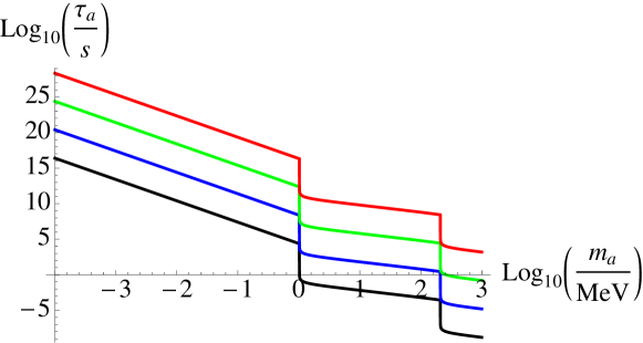
Figure 1: Theoretical predictions for the R-axion lifetime with various values of $f_{a}$. Black, blue, green and red lines correspond to $f_{a}=10^{6}$GeV, $10^{8}$GeV, $10^{10}$GeV, and $10^{12}$GeV, respectively. Here we use $\tan\beta=30$.

We can see that the lifetime of R-axions becomes longer for smaller $m_{a}$ and larger $f_{a}$. We can also see that the decay channels to electrons opens at $m_{a}\simeq 1$ MeV and to muons at $m_{a}\simeq 200$ MeV and the R-axion lifetime becomes shorter.

III R-axion production in the early Universe

Let us consider the cosmology of the spontaneous R-symmetry breaking model focusing on the R-axion production and evaluate the R-axion abundance. We consider the case where $U(1)_{R}$ is restored due to some additional mass terms such as the Hubble induced mass or thermal mass in the early Universe. After some epoch, $X$ field is destabilized as the additional mass term decreases and acquires vacuum expectation value $\chi=f_{a}$. Since the approximate $U(1)_{R}$ symmetry breaks spontaneously at that time, (unstable) cosmic strings are formed by the Kibble-Zurek mechanism. The long cosmic strings in a Hubble volume intersect each other and generates closed string loops. These closed string loops shrink with emitting R-axions. As a consequence, the cosmic string network enters the scaling regime. As the Hubble parameter decreases, the explicitly R-symmetry breaking term in the potential becomes no longer irrelevant to the dynamics of the system and the string network turns to the string-wall system where domain walls are attached to cosmic strings Sikivie:1982qv ; Hiramatsu:2012gg . The string-wall networks are unstable and annihilate when the domain wall tension becomes comparable to that of cosmic strings. The energy stored in the string-wall system turns to R-axion particles. The fate of R-axions produced from the cosmic string loops and the string-wall system as well as the scattering of thermal plasma and the vacuum misalignment is determined by the lifetime of R-axions, which, then, constrain the model parameters of spontaneous R-symmetry breaking models. In the following, we estimate the R-axion abundance from each source. We will examine the cosmological constraints in Sec. IV.

III.1 R-axion production from vacuum misalignment

First we evaluate the energy density of the coherent oscillation of the R-axion field Dine:1982ah . After the spontaneous R-symmetry breaking phase transition, the R-axion field acquires some initial value, $a_{i}$, and keeps its position after a while due to large Hubble friction. When the Hubble parameter decreases to the R-axion mass,

$$H(t_{\rm osc})=m_{a},$$ (18)

the R-axion field starts to oscillate. Here the subscription “osc” indicates that the parameter or variable is evaluated at the onset of the R-axion oscillation. The energy density of the oscillating R-axion $\rho_{a,{\rm o}}$ is given by

$$\rho_{a,{\rm o}}(t_{\rm osc})=\frac{1}{2}m_{a}^{2}a_{i}^{2}.$$ (19)

If the R-symmetry is broken after inflation, the initial value of R-axion distributes randomly from $-\sqrt{2}\pi f_{a}$ to $\sqrt{2}\pi f_{a}$ since the correlation length of R-axion becomes much shorter than the Hubble length at the onset of the R-axion oscillation. Therefore, we estimate the mean value of $a_{i}$ as

$$\langle a_{i}^{2}\rangle=\frac{1}{2\sqrt{2}\pi f_{a}}\int_{-\sqrt{2}\pi f_{a}}^{\sqrt{2}\pi f_{a}}a_{i}^{2}da_{i}=\frac{2\pi^{2}f_{a}^{2}}{3}.$$ (20)

Since the energy density of R-axion oscillation decreases as $a^{-3}$, the quantity $\rho_{a}/s$ is conserved as long as there are no entropy production, where $s$ is the entropy density. Therefore, we characterize the axion abundance by this quantity as

$$\frac{\rho_{a,{\rm o}}}{s}\simeq\left\{\begin{array}[]{ll}\dfrac{15}{2g_{*s}(T_{\rm osc})}\dfrac{m_{a}^{2}f_{a}^{2}}{T_{\rm osc}^{3}},&\text{for}\quad H_{\rm osc}<H_{R}\\ \dfrac{\pi^{2}}{12}\dfrac{g_{*}(T_{R})}{g_{*s}(T_{R})}\left(\dfrac{f_{a}}{M_{\rm pl}}\right)^{2}T_{R},&\text{for}\quad H_{\rm osc}>H_{R}\end{array}\right.$$ (21)

where $g_{*}$ and $g_{*s}$ are (effective) relativistic degrees of freedom for energy density and entropy, respectively, and the subscript “$R$” represents that the parameter or variable is evaluated at reheating. Note that $T_{\rm osc}$ is given by

$$T_{\rm osc}=\left(\frac{90}{\pi^{2}g_{*}(T_{\rm osc})}\right)^{1/4}m_{a}^{1/2}M_{\rm pl}^{1/2}\simeq 2.2\times 10^{7}{\rm GeV}\left(\frac{m_{a}}{1{\rm MeV}}\right)^{1/2}.$$ (22)

Here we assume that the scale factor increases like matter dominated era during inflaton oscillation dominated era and take into account the dilution until the inflaton decay or reheating when $H_{\rm osc}>H_{R}$.

III.2 R-axion production from global cosmic strings

Next we evaluate the energy density of R-axions radiated from the cosmic string loops Davis:1986xc ; Yamaguchi:1998gx following the discussion in Appendix B of Ref. Hiramatsu:2010yu . When the R-string network enters the scaling regime, the energy density of the long R-strings are estimated as

$$\rho_{\infty}(t)=\frac{2\pi\xi}{t^{2}}f_{a}^{2}\ln\left(\frac{t/\sqrt{\xi}}{d_{\rm string}}\right).$$ (23)

Here the scaling parameter $\xi\simeq 0.9$ Hiramatsu:2010yu ; Yamaguchi:2002zv represents the mean number of strings in a Hubble volume and $d_{\rm string}\simeq\lambda^{-1/2}f_{a}^{-1}$ represents the core width of R-string. Note that the line energy density or the tension of R-string is given by stringreveiw

$$\mu_{\rm string}\simeq 2\pi f_{a}^{2}\ln\left(\frac{t/\sqrt{\xi}}{d_{\rm string}}\right).$$ (24)

Assuming all the energy loss of long R-strings is converted into R-axion particles through the string loops, we obtain the evolution equations

$$\frac{d\rho_{\infty}(t)}{dt} =-2H\rho_{\infty}(t)-\Gamma_{\rm em}(t),$$ (25)

$$\frac{d\rho_{a,{\rm str}}(t)}{dt} =-4H\rho_{a,\rm str}(t)+\Gamma_{\rm em}(t),$$ (26)

where the energy emission rate from the string loops,

$$\Gamma_{\rm em}(t)=\frac{2\pi\xi f_{a}^{2}}{t^{3}}\times\left\{\begin{array}[]{ll}\left(\ln\left(\dfrac{t/\sqrt{\xi}}{d_{\rm string}}\right)-1\right),&\text{for RD}\\ \left(\dfrac{2}{3}\ln\left(\dfrac{t/\sqrt{\xi}}{d_{\rm string}}\right)-1\right).&\text{for MD}\end{array}\right.$$ (27)

Here we assume that R-axion particles released from cosmic string loops are relativistic. Since the mean comoving momentum of radiated R-axion can be evaluated as

$$\frac{k_{a,{\rm str}}(t)}{R(t)}=\frac{2\pi\epsilon}{t},$$ (28)

with the constant $\epsilon\simeq 0.25$ Hiramatsu:2010yu ; Yamaguchi:1998gx , we can estimate the number density of radiated R-axions as

$$n_{a,{\rm str}}(t) =\frac{1}{R(t)^{3}}\int_{t_{*}}^{t}dt^{\prime}\frac{R^{4}(t^{\prime})}{k_{a,{\rm str}}(t^{\prime})}\Gamma_{\rm em}(t^{\prime})$$

$$\simeq\frac{2\xi f_{a}^{2}}{\epsilon t}\times\left\{\begin{array}[]{ll}\left(\ln\left(\dfrac{t/\sqrt{\xi}}{d_{\rm string}}\right)-3\right),&\text{for}\quad t>t_{R}\\ \dfrac{1}{3}\left(\ln\left(\dfrac{t/\sqrt{\xi}}{d_{\rm string}}\right)-\dfrac{5}{2}\right).&\text{for}\quad t<t_{R}\end{array}\right.$$ (31)

Here $t_{*}$ is the time when the R-string network enters the scaling regime.

When the Hubble parameter becomes comparable to the R-axion mass and R-symmetry breaking mass term becomes no longer irrelevant, $t=t_{\rm osc}$, string-wall system forms and R-axion emission from R-string loops stops. We can evaluate the resultant number density of R-axions from the R-string loops as

$$n_{a,{\rm str}}(t_{\rm osc})=\frac{\xi m_{a}f_{a}^{2}}{\epsilon}\times\left\{\begin{array}[]{ll}4\left(\ln\left(\dfrac{1}{2m_{a}\sqrt{\xi}d_{\rm string}}\right)-3\right),&\text{for}\quad H_{\rm osc}<H_{R}\\ \left(\ln\left(\dfrac{2}{3m_{a}\sqrt{\xi}d_{\rm string}}\right)-\dfrac{5}{2}\right).&\text{for}\quad H_{\rm osc}>H_{R}\end{array}\right.$$ (32)

The radiated R-axions become nonrelativistic after some epoch. Therefore, we can approximate the R-axion energy density as $\rho_{a,{\rm str}}=m_{a}n_{a,{\rm str}}$ and the R-axion energy-to-entropy ratio as

$$\frac{\rho_{a,{\rm str}}}{s}=\left\{\begin{array}[]{ll}\dfrac{90}{\pi^{2}}\dfrac{\xi}{g_{*s}(T_{\rm osc})\epsilon}\dfrac{m_{a}^{2}f_{a}^{2}}{T_{\rm osc}^{3}}\left(\ln\left(\dfrac{1}{2m_{a}\sqrt{\xi}d_{\rm string}}\right)-3\right),&\text{for}\quad H_{\rm osc}<H_{R}\\ \dfrac{g_{*}(T_{R})\xi}{4g_{*s}(T_{R})\epsilon}\left(\dfrac{f_{a}}{M_{\rm pl}}\right)^{2}T_{R}\left(\ln\left(\dfrac{2}{3m_{a}\sqrt{\xi}d_{\rm string}}\right)-\dfrac{5}{2}\right).&\text{for}\quad H_{\rm osc}>H_{R}\end{array}\right.$$ (33)

III.3 R-axion production from string-wall system

Let us evaluate the energy density of R-axions from the string-wall system annihilation Sikivie:1982qv ; Hiramatsu:2012gg . At $t\simeq t_{\rm osc}$, the explicitly R-symmetry breaking term in the potential (2) becomes no longer irrelevant, and string-wall system forms. The surface mass density of domain walls are estimated as stringreveiw

$$\sigma_{\rm wall}=16m_{a}f_{a}^{2}.$$ (34)

When the tension of domain walls dominates that of strings,

$$\sigma_{\rm wall}=\frac{\mu_{\rm string}}{t}\Leftrightarrow t\ln\left(\frac{d_{\rm string}}{t/\sqrt{\xi}}\right)=\frac{\pi}{8}m_{a}^{-1},$$ (35)

the string-wall system annihilates. As following the discussion in Ref. Hiramatsu:2012gg , we assume that the energy stored in the string-wall system released to R-axion particles. Thus, we evaluate the number density of R-axions as

$$n_{a,{\rm sw}}(t) =\frac{\rho_{\rm wall}(t_{\rm osc})+\rho_{\infty}(t_{\rm osc})}{\omega_{a}}\left(\frac{R(t_{\rm osc})}{R(t)}\right)^{3}$$

$$=\frac{1}{\alpha_{w}m_{a}}\left({\cal A}\frac{\sigma_{\rm wall}}{t_{\rm osc}}+\xi\frac{\mu_{\rm string}(t_{\rm osc})}{t_{\rm osc}^{2}}\right)\left(\frac{R(t_{\rm osc})}{R(t)}\right)^{3},$$ (36)

where $\omega_{a}=\alpha_{w}m_{a}$ is the average energy of radiated axions and ${\cal A}\equiv\rho_{\rm wall}t/\sigma_{\rm wall}\simeq 0.5$ Hiramatsu:2012gg is the area parameter of domain walls. The radiated R-axions become eventually nonrelativistic and hence we can evaluate the energy-to-entropy ratio as

$$\frac{\rho_{a,{\rm sw}}}{s} =\frac{m_{a}n_{a,{\rm sw}}}{s}=\left\{\begin{array}[]{ll}\dfrac{180}{\pi^{2}g_{*s}(T_{\rm osc})\alpha_{w}}\dfrac{m_{a}^{2}f_{a}^{2}}{T_{\rm osc}^{3}}\left(4{\cal A}+\pi\xi\ln\left(\dfrac{1}{2m_{a}\sqrt{\xi}d_{\rm string}}\right)\right),&\text{for}\quad H_{\rm osc}<H_{R}\\ \dfrac{g_{*}(T_{R})}{4g_{*s}(T_{R})\alpha_{w}}\left(\dfrac{f_{a}}{M_{\rm pl}}\right)^{2}T_{R}\left(24{\cal A}+\dfrac{9\pi}{2}\xi\ln\left(\dfrac{2}{3m_{a}\sqrt{\xi}d_{\rm string}}\right)\right).&\text{for}\quad H_{\rm osc}>H_{R}\end{array}\right.$$ (39)

Noting that the logarithmic factor is evaluated as $\ln(1/m_{a}\sqrt{\xi}d_{\rm string})\simeq\ln(\sqrt{\lambda/\xi}(f_{a}/m_{a}))=30$ for $f_{a}\simeq 10^{10}$ GeV and $m_{a}\simeq$ 1 MeV, hereafter we approximate the R-axion abundance from R-axion dynamics, i.e., the coherent oscillation, the decay of cosmic string loops, and the decay of the string-wall system,

$$\frac{\rho_{a,{\rm dyn}}}{s} \equiv\frac{\rho_{a,{\rm o}}+\rho_{a,{\rm str}}+\rho_{a,{\rm sw}}}{s}=\left\{\begin{array}[]{ll}K_{1}\dfrac{m_{a}^{2}f_{a}^{2}}{T_{\rm osc}^{3}},&\text{for}\quad H_{\rm osc}<H_{R}\\ K_{2}\left(\dfrac{f_{a}}{M_{\rm pl}}\right)^{2}T_{R},&\text{for}\quad H_{\rm osc}>H_{R}\end{array}\right.$$ (42)

$$\simeq\left\{\begin{array}[]{ll}9.4\times 10^{-9}{\rm GeV}K_{1}\left(\dfrac{m_{a}}{1{\rm MeV}}\right)^{1/2}\left(\dfrac{f_{a}}{10^{10}{\rm GeV}}\right)^{2},&\text{for}\quad H_{\rm osc}<H_{R}\\ 1.7\times 10^{-11}{\rm GeV}K_{2}\left(\dfrac{f_{a}}{10^{10}{\rm GeV}}\right)^{2}\left(\dfrac{T_{R}}{10^{6}{\rm GeV}}\right),&\text{for}\quad H_{\rm osc}>H_{R}\end{array}\right.$$ (45)

where $K_{1}\simeq{\cal O}(1)$ and $K_{2}\simeq{\cal O}(10)$ are numerical parameters.

III.4 R-axion production from thermal bath

We have estimated the abundance of R-axions generated from their dynamics. We should also take into account that generated from other sources. Here we evaluate the R-axion abundance from thermal bath. The R-axion abundance from R-saxion decay is discussed in Appendix B and is generally negligible.

R-axions are produced in the thermal plasma from (mainly) gluon scattering, $gg\rightarrow ag$. Since the gluon-axion interaction comes from the anomaly term,

$${\cal L}=\frac{C_{g}g_{s}^{2}}{32\pi^{2}f_{a}}aG^{b}_{\mu\nu}{\tilde{G}}^{b\mu\nu},$$ (46)

with $C_{g}$ being the model dependent anomalous coefficient and $g_{s}$ being the strong gauge coupling, the R-axion abundance is calculated as Masso:2002np ; Sikivie:2006ni ; Graf:2010tv ,

$$\frac{\rho_{a,{\rm th}}}{s}\simeq 2.0\times 10^{-6}{\rm GeV}g_{s}^{6}C_{g}^{2}\left(\frac{m_{a}}{1{\rm MeV}}\right)\left(\frac{10^{10}{\rm GeV}}{f_{a}}\right)^{2}\left(\frac{T_{R}}{10^{6}{\rm GeV}}\right).$$ (47)

Note that R-axions are thermalized once if the reheating temperature is high enough,

$$T_{R}>T_{D}\simeq 10^{6}{\rm GeV}g_{s}^{-6}C_{g}^{-2}\left(\frac{f_{a}}{10^{10}{\rm GeV}}\right)^{2},$$ (48)

where $T_{D}$ is R-axion decoupling temperature. In this case, the R-axion abundance is evaluated as

$$\frac{\rho_{a,{\rm th}}}{s}\simeq 2.6\times 10^{-6}{\rm GeV}\left(\frac{m_{a}}{1{\rm MeV}}\right).$$ (49)

Note that R-axion is produced thermally only if $T_{R}\gtrsim m_{a}$ is satisfied.

As a result, the total R-axion abundance in the early Universe is evaluated by the sum of these contributions and given by

$$\frac{\rho_{a}}{s}=\dfrac{\rho_{a,{\rm dyn}}}{s}+\dfrac{\rho_{a,{\rm th}}}{s}.$$ (50)

In Fig. 2, we show the theoretical predictions for the R-axion to entropy ratio with $f_{a}=10^{6}$GeV, $10^{8}$GeV, $10^{10}$GeV, and $10^{12}$GeV. Here the solid lines represent contribution from the thermal production (Eqs. (47) and (49)) and dashed ones represent the R-axion dynamics (Eq. (45)) with $K_{1}=1$, $K_{2}=20$, respectively. Black, blue, green and red lines correspond to $T_{R}=10^{-2}$GeV, $1$GeV, $10^{3}$GeV, and $10^{6}$GeV, respectively. In the case of $T_{R}>T_{D}$, R-axion abundance from thermal production is independent of $T_{R}$. We can see that the contribution from the R-string dynamics and other R-axion dynamics generally dominates for $f_{a}\gtrsim 10^{12}$GeV and smaller $m_{a}$. Vice versa, thermal R-axion production dominates for $f_{a}\lesssim 10^{12}$GeV. Anyway, we will compare the total R-axion abundance expressed in Eq. (50), including those from R-string dynamics and thermally produced ones, to the cosmological constraints discussed in the next section and will give the constraints on the model parameters.

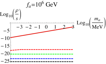
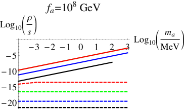
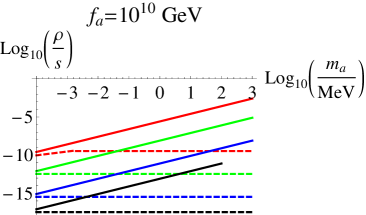
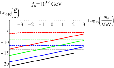
Figure 2: Theoretical predictions for the R-axion to entropy ratio with $f_{a}=10^{6}$GeV, $10^{8}$GeV, $10^{10}$GeV, and $10^{12}$GeV. The solid lines represent contribution from the thermal production (Eqs. (47) and (49)) and the dashed ones represent the R-axion dynamics (Eq. (45)) with $K_{1}=1$, $K_{2}=20$. Black, blue, green and red lines correspond to $T_{R}=10^{-2}$GeV, $1$GeV, $10^{3}$GeV, and $10^{6}$GeV, respectively.

IV Cosmological constraints from R-axion

Now we consider the generic constraints of the R-symmetry breaking model from cosmology. One may think that the model with long-lived R-axions is safe if they never dominate the energy density of the Universe or R-axions are responsible for the dark matter in the present Universe. However, even if they are subdominant component of the Universe, their (partial) decay is constrained by several cosmic/astrophysical observations depending on their abundance Kawasaki:2007mk . Since we have evaluated the R-axion abundance and its lifetime, we can constrain the model from various observations. As we will see, strong constraints for the model parameters are imposed.

IV.1 Cosmological constraints on axion abundance

Let us see the various constraints of R-axion abundance from cosmology and astrophysical observations. We will compare all these constraints on the R-axion abundance to that evaluated in the previous section, especially in Eq. (50) and translate them in the constraints on the R-axion model parameters in the next subsection. Note that our cosmological constraints are basically irrelevant to what is the dominant source of R-axions, but relevant to the total R-axion abundance in Eq.(41).

IV.1.1 Big Bang Nucleosynthesis

The R-axion decay into photon or electron (radiative decay) after the Big Bang Nucleosynthesis (BBN) epoch may break the light elements and the R-axion abundance is constrained Kawasaki:2004qu . The radiative decay of R-axion causes photo-dissociation process of light elements and changes the light elements abundance. We can read off the constraint on the R-axion abundance at its decay from Ref. Kawasaki:2004qu as

$$B_{\rm r}\frac{\rho_{a}}{s}\lesssim\left\{\begin{array}[]{ll}10^{-8}{\rm GeV}\left(\dfrac{\tau_{a}}{10^{4}{\rm s}}\right)^{-2},&\text{for}\quad 10^{4}{\rm s}<\tau_{a}<10^{7}{\rm s}\\ 10^{-14}{\rm GeV},&\text{for}\quad 10^{7}{\rm s}<\tau_{a}<10^{12}{\rm s}\end{array}\right.$$ (51)

where $B_{\rm r}$ is the radiative branching ratio. Note that this effect is negligible if the energy of the injected photons is so small that they cannot destroy the light elements. Thus, we here impose a condition for this constraint to be effective,

$$m_{a}\gtrsim 4.5{\rm MeV},$$ (52)

which corresponds to the threshold energy for the deuteron destruction process, $D+\gamma\rightarrow n+p$.

IV.1.2 Cosmic microwave background distortion

The radiative decay of R-axion before the recombination may distort the blackbody spectrum of CMB. After the double-Compton scattering freezes out at $t\simeq 10^{6}$ s, energy injections generate nonzero chemical potential $\mu$ of the CMB spectrum, which imposes the constraint from the blackbody spectrum distortion of CMB. Energy injections after $t\simeq 10^{9}$ s, when the Compton scattering is no longer in thermal equilibrium, thermalize electron, which causes the Sunyaev-Zel’dovich (SZ) effect. Since the SZ effect is constrained by the Compton $y$-parameter, we can impose a constraint on the R-axion abundance.

The COBE FIRAS measurement Fixsen:1996nj constrains the CMB distortion as

$$|\mu|\lesssim 9\times 10^{-5},\quad y\lesssim 1.2\times 10^{-5}.$$ (53)

Since the injected energy is related to these parameters as Ellis:1990nb ; Hu:1993gc

$$\frac{\delta\rho_{\gamma}}{\rho_{\gamma}} \sim 0.714\mu,\quad\text{for}\quad 10^{6}{\rm s}<\tau_{a}<10^{9}{\rm s}$$ (54)

$$\frac{\delta\rho_{\gamma}}{\rho_{\gamma}} \sim 4y,\quad\text{for}\quad 10^{9}{\rm s}<\tau_{a}<10^{13}{\rm s}$$ (55)

the constraints on the R-axion abundance is given by

$$B_{\rm r}\frac{\rho_{a}}{s}\lesssim 10^{-12}{\rm GeV}\left(\frac{10^{9}{\rm s}}{\tau_{a}}\right)^{1/2}\quad\text{for}\quad 10^{6}{\rm s}<\tau_{a}<10^{13}{\rm s}$$ (56)

depending on its life time. Note that $\mu$ and $y$-parameters impose almost the same constraint on the R-axion abundance at its decay.

IV.1.3 Diffuse X-ray and $\gamma$-ray background

The R-axion decay to photons after recombination, $t>10^{13}$ s, may be constrained from the diffuse X-ray and $\gamma$-ray background observation. Photons with energy $1{\rm keV}<E_{\gamma}<1{\rm TeV}$ rarely scatter with the CMB photons and intergalactic medium. Therefore, the photons produced from the R-axion decay in the “transparency window” Chen:2003gz ,

$$\tau_{a}\gtrsim\left\{\begin{array}[]{ll}10^{19}\ {\rm s}\left(\dfrac{m_{a}}{1\ {\rm keV}}\right)^{-2},&\text{for}\quad 1\ {\rm keV}\lesssim m_{a}\lesssim 100\ {\rm keV}\\ 4\times 10^{14}\ {\rm s},&\text{for}\quad 100\ {\rm keV}\lesssim m_{a}\lesssim 2.5\ {\rm MeV}\\ 10^{13}\ {\rm s}\left(\dfrac{m_{a}}{100\ {\rm MeV}}\right)^{-1},&\text{for}\quad 2.5\ {\rm MeV}\lesssim m_{a}\lesssim 100\ {\rm MeV}\\ 10^{13}{\rm s},&\text{for}\quad 100\ {\rm MeV}\lesssim m_{a}\lesssim 10\ {\rm GeV}\end{array}\right.$$ (57)

propagate through the Universe and can be detected as diffuse background.

The flux of the extragalactic diffuse photons is roughly given by

$$F^{\rm obs}_{\gamma}(E)/{\rm cm}^{-2}{\rm s}^{-1}{\rm str}^{-1}\simeq\left\{\begin{array}[]{ll}2\times\left(\dfrac{E}{\rm keV}\right)^{-0.4},&0.25{\rm keV}<E<10{\rm keV}\\ \dfrac{3}{(E/30{\rm keV})^{0.3}+(E/30{\rm keV})^{1.9}},&10{\rm keV}<E<800{\rm keV}\\ 5.0\times 10^{-3}\left(\dfrac{E}{\rm MeV}\right)^{-1.4},&800{\rm keV}<E<30{\rm MeV}\\ 1.7\times 10^{-5}\left(\dfrac{E}{100{\rm MeV}}\right)^{-1.1},&30{\rm MeV}<E<100{\rm MeV}\\ 1.45\times 10^{-5}\left(\dfrac{E}{100{\rm MeV}}\right)^{-1.4}.&100{\rm MeV}<E<100{\rm GeV}\end{array}\right.$$ (58)

Here we applied the observational results of ASCA ASCA for 0.25-10 keV, HEAO HEAO for 25 keV- 800 keV, COMPTEL 1998PhDT3K for 800 keV-30 MeV, EGRET Sreekumar:1997un for 30 - 100 MeV, and Fermi Abdo:2010nz for 100 MeV-100 GeV. Note that we have taken into account the resolved source of diffuse X-ray background Worsley:2004tc ; Hickox:2005dz and used the fitting formula derived in Ref.  CXBfit .

The flux of photons produced from the R-axion decay can be approximated as

$$F_{\gamma}(E)\simeq B_{\gamma}\times\left\{\begin{array}[]{ll}\dfrac{n_{a,0}}{2\pi\tau_{a}H_{0}},&\text{for}\quad\tau_{a}>t_{0}\\ \dfrac{3n_{a,{\rm dec}}}{4\pi}\dfrac{s_{0}}{s_{\rm dec}},&\text{for}\quad\tau_{a}<t_{0}\end{array}\right.$$ (59)

where the subscriptions “0” and “dec” indicate that the parameter or variable is evaluated at the present and the R-axion decay time, respectively, and $B_{\gamma}$ is the branching ratio to photons. Note that the energy of photons should be evaluated at $E=m_{a}/2$ for $\tau_{a}>t_{0}$ and $E=(3H_{0}\tau_{a}\sqrt{\Omega_{\rm m}}/2)^{2/3}(m_{a}/2)$ for $\tau_{a}<t_{0}$, taking into account of the redshift of the photons. Then, the abundance of the R-axions are constrained from the constraint $F_{\gamma}(E)<F_{\gamma}^{\rm obs}$ as

$$B_{\gamma}\frac{\rho_{a}}{s}\lesssim\left\{\begin{array}[]{ll}2.4h\times 10^{-18}{\rm GeV}\left(\dfrac{m_{a}}{1{\rm MeV}}\right)\left(\dfrac{\tau_{a}}{10^{18}{\rm s}}\right)\left(\dfrac{F_{\gamma}^{\rm obs}(m_{a}/2)}{10^{-2}{\rm cm}^{-2}{\rm s}^{-2}}\right),&\text{for}\quad\tau_{a}>t_{0}\\ 4.8\times 10^{-19}{\rm GeV}\left(\dfrac{m_{a}}{1{\rm MeV}}\right)\left(\dfrac{F_{\gamma}^{\rm obs}(E)}{10^{-2}{\rm cm}^{-2}{\rm s}^{-2}}\right),&\text{for}\quad\tau_{a}<t_{0}\end{array}\right.$$ (60)

where $h\equiv H_{0}/(100\ {\rm km}\ {\rm sec}^{-1}{\rm Mpc}^{-1})$ and $H_{0}$ is the present Hubble parameter.

IV.1.4 Reionization

The radiative decay of R-axion after recombination is also constrained from reionization. If the energy of injected photons is relatively small, they are redshifted and interact with intergalactic medium. Then, the intergalactic medium is partially ionized and the R-axion decay is regarded as an additional source of reionization. To be consistent with the observation of the optical depth to the last scattering surface, the R-axion abundance should be small enough. Assuming that the one-third of the energy of photons produced from R-axion decay that leaves the transparency window is converted to the ionization of the intergalactic medium, the R-axion abundance can be constrained from the inequality in Ref. Chen:2003gz ; Zhang:2007zzh ,

$$\log_{10}\zeta\lesssim\left\{\begin{array}[]{ll}6.77+3.96275x+0.25858x^{2}+0.00445x^{3},&-17<x<-13\\ -24.75-x,&x<-17\end{array}\right.$$ (61)

where

$$\zeta\equiv B_{\rm r}\rho_{a}/\rho_{\rm baryon}|_{\rm dec}=0.43\times 10^{10}{\rm GeV}^{-1}\left(\frac{\Omega_{b}h^{2}}{0.022}\right)^{-1}\frac{B_{\rm r}\rho_{a}}{s},$$ (62)

and $x\equiv\log_{\rm 10}(\Gamma/{\rm s}^{-1})=-\log_{\rm 10}(\tau_{a}/{\rm s})$. Here $\Omega_{b}$ denotes the present density parameter of the baryonic matter. This constraint is complementary to that from the diffuse X-ray and $\gamma$-ray background.

IV.1.5 Dark matter abundance

If the lifetime of R-axions is longer than the present time $t_{0}$, most of R-axions remain the present Universe and contribute to the dark matter of the Universe. Thus, we can constrain the R-axion abundance in order not to exceed that of the dark matter. In terms of the energy-to-entropy ratio, the R-axion abundance is constrained as Komatsu:2010fb

$$\frac{\rho_{a}}{s}<4.7\times 10^{-10}{\rm GeV}\left(\frac{\Omega_{m}h^{2}}{0.13}\right).$$ (63)

IV.2 Constraints on model parameters

Now we are ready to show cosmological constraints for spontaneous R-symmetry breaking models. In Fig.3, we show the constraints on the model parameters, $m_{a}$ and $f_{a}$ coming from various conditions argued in the previous subsection. Each colored region is excluded and white region is allowed. As a reference, we also show lines of gravitino mass. Upper dotted lines and lower ones represent $m_{3/2}=1$keV, $m_{3/2}=1$eV, respectively. Here we focus on the region $f_{a}>10^{6}$ GeV since smaller $f_{a}$ is forbidden from laboratory experiments such as rare decays of $K^{+}$ or $B^{0}$ Andreas:2010ms .

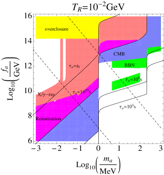
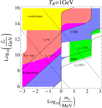
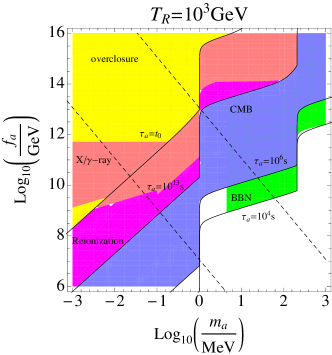
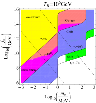
Figure 3: Cosmological constraints on the model parameters, $m_{a}$ and $f_{a}$ with $T_{R}=10^{-2}$GeV, $1$GeV, $10^{3}$GeV, and $10^{6}$GeV. Each colored region is excluded and white region is allowed. Upper dotted lines and lower ones represent $m_{3/2}=1$keV and $m_{3/2}=1$eV. Solid black lines represents the contour lines of equal R-axion lifetime, $\tau_{a}=10^{4},10^{6},10^{13}$ sec and $t_{0}$, respectively.

For the higher reheating temperature, $T_{R}\gtrsim 10^{2}$ GeV, all the parameter space where R-axions decay at $t>10^{6}$ sec is ruled out regardless of reheating temperature, which comes from the CMB constraint. For $m_{a}<1$ MeV, it corresponds to $f_{a}\lesssim 10^{7}{\rm GeV}(f_{a}/1{\rm MeV})^{3/2}$, and $1{\rm MeV}<m_{a}<4.5$ MeV, it corresponds to $f_{a}<10^{9.5}{\rm GeV}(f_{a}/1{\rm MeV})^{1/2}$. For $m_{a}>4.5$ MeV, the BBN constraint opens and all the parameter space where the R-axion lifetime is $t>10^{4}$ sec is ruled out, again, regardless of reheating temeperature. For $4.5{\rm MeV}<m_{a}<200$ MeV, it corresponds to $f_{a}\lesssim 10^{9}{\rm GeV}(f_{a}/10{\rm MeV})^{1/2}$, and for $m_{a}>200$ MeV, it corresponds to $f_{a}<10^{12}{\rm GeV}(f_{a}/200{\rm MeV})^{1/2}$. This is because R-axions are inevitably produced so much that cannot pass any constraints discussed above, especially, the BBN and CMB constraints. Short-lived R-axion is allowed because any entropy production before is not forbidden and there are no cosmological constraints.

On the other hand, for the smaller reheating temperature, $T_{R}\lesssim 10^{2}$ GeV, several parameter space where R-axions decay later is allowed. This can be understood from Eqs. (45) and (47). For larger $f_{a}$, nonthermal production is dominant and the R-axion abundance is expressed as $\rho_{a}/s\propto f_{a}^{2}$, whereas thermal production, which depends on $f_{a}$ as $\rho_{a}\propto f_{a}^{-2}$, dominates for smaller $f_{a}$. Thus, the R-axion abundance takes its lower value at $f_{a}\sim 10^{11-12}$ GeV. As a result, allowed parameter region appears at $m_{a}\sim 10$ keV and 1-100 MeV for $f_{a}\sim 10^{12}$ GeV and $T_{R}\sim 10^{-2}-1$ GeV.

One may regard that there is a parameter region where R-axions can be dark matter for smaller reheating temperature, $f_{a}\sim 10^{14}$ GeV. However, in this parameter region, R-saxion mass is considerably small, $m_{s}\lesssim 1$ MeV for a naive model discussed in Sec. II. For the point of view of vacuum selection and R-string stability OurpaperI , this requires unacceptably small messenger mass. Therefore, we conclude that an ingenious model building is necessary for R-axions to be dark matter of the present Universe.

Thus far, we did not take into account constraints from R-axinos or gravitinos. Gravitinos are produced from gluino scattering in thermal plasma and their abundance is evaluated as Kawasaki:2004qu ; Kawasaki:2004yh ,

$$\frac{\rho_{3/2}}{s}\simeq 9.5\times 10^{-8}{\rm GeV}\times\left(\frac{m_{\tilde{g}}}{1.5{\rm TeV}}\right)^{2}\left(\frac{m_{3/2}}{15{\rm GeV}}\right)^{-1}\left(\frac{T_{R}}{10^{10}{\rm GeV}}\right),$$ (64)

where $m_{\tilde{g}}$ is the gaugino mass. Since gravitinos are stable in this case, gravitino abundance is constrained from dark matter abundance (Eq. (63)). As a result, depending on the gaugino mass, another stringent constraint is imposed for model parameters in higher reheating temperature case $T_{R}\gtrsim 10$ GeV: Smaller $f_{a}$ and $m_{a}$ would be forbidden.

In summary, we have shown that spontaneous R-symmetry breaking models are severely constrained from cosmological considerations and generally long-lived R-axions are forbidden. In order to avoid that, careful model building and smaller reheating temperature are required.

V Discussion

We have studied general cosmological constraints on spontaneous R-symmetry breaking models. We estimated the abundance of R-axion produced firstly via their dynamics such as coherent oscillation and decay of cosmic string/wall system, and secondly via thermal scattering process from gluon-axion interaction. It is interesting that R-axion production from R-string and wall systems are large enough and can be dominant in some parameter region. Basically the models were motivated by gauge mediation, gravitino as well as R-axion are relatively light. Therefore, R-axion tends to be long-lived. The conditions for the R-axion density coming from BBN, X-ray/$\gamma$-ray background, reionization and overclosure severely constrain the scale of R-symmetry breaking. As a result, smaller R-symmetry breaking scale and SUSY-breaking scale are disfavored from cosmological constraints. In the point of view of gauge mediation, this result weakens its motivation, but is consistent with the recent LHC results with 125 GeV Higgs-like boson and without SUSY particles SUSYiloHiggs .

It would be interesting to study further constraints for R-axion with relatively large mass. When the R-axion mass is larger than $1$ GeV, various decay channels to hadronic particle open. We expect that weaker but non-negligible constraints for large decay constant will be imposed, thought analysis would become involved.

A phenomenologically viable model with long-lived R-axions can be constructed by introducing a mechanism diluting the R-axion density in the early universe. Although our primary interest was gauge mediation models, it would be easy to apply our analysis the closely related situations such as spontaneous R-symmetry breaking in thermal inflation models Thermal0 .

In this paper, we have not explicitly shown a mechanism of vacuum selection of false vacuum. Existence of the R-string and walls are highly depend on the scenario of the early stage of universe. Also, as mentioned in the Introduction, imhomogenious vacuum decay by impurities such as a cosmic string depends on the details of the scenario OurpaperI . So it may be useful to show an explicit example of full scenario and study R-axion cosmology in detail. This is beyond the scope of our study, so we will leave it as a future work.

Appendix A Higgs sector

In this appendix, we show the Higgs sector and its mixing with the R-axion following Ref. Goh:2008xz . Here, we concentrate on the neutral components, $H_{u}^{0}$ and $H^{0}_{d}$, of the Higgs sector in the minimal supersymmetric standard model. The R-axion appears through the so-called B-term. Then, the relevant terms in their scalar potential are given by

$$V = (|\mu|^{2}+m^{2}_{H_{u}})|H^{0}_{u}|^{2}+(|\mu|^{2}+m^{2}_{H_{d}})|H^{0}_{d}|^{2}+\frac{1}{8}(g^{2}+g^{\prime 2})(|H^{0}_{u}|^{2}-|H^{0}_{d}|^{2})^{2}$$ (65)

$$-(e^{ia/(\sqrt{2}f_{a})}B\mu H_{u}^{0}H_{d}^{0}+c.c.),$$

where $\mu$ is the supersymmetric mass, originated from the $\mu$ term, $m^{2}_{H_{u}}$ and $m^{2}_{H_{d}}$ are soft SUSY breaking masses squared for $H_{u}$ and $H_{d}$, and $B\mu$ is the SUSY breaking B-term. The B-term has an R-charge, and the axion appears there.

At the potential minimum, the Higgs fields develop their vacuum expectation values and the electroweak symmetry is broken. Around the vacuum, we decompose the neutral Higgs fields as

$$H^{0}_{u}=\frac{1}{\sqrt{2}}(v_{u}+\rho_{u})e^{i\xi_{u}/v_{u}},\qquad H^{0}_{d}=\frac{1}{\sqrt{2}}(v_{d}+\rho_{d})e^{i\xi_{d}/v_{d}},$$ (66)

where $v_{u}$ and $v_{d}$ are VEVs of $H^{0}_{u}$ and $H^{0}_{d}$. We denote $v^{2}=v_{u}^{2}+v_{d}^{2}$, which is related to the $Z$-boson mass $m_{Z}$ as $v^{2}=4m_{Z}^{2}/(g^{2}+g^{\prime 2})=(246)^{2}$ (GeV)². Also we denote their ratio as

$$\tan\beta=\frac{v_{u}}{v_{d}}.$$ (67)

Furthermore, the stationary conditions,

$$\frac{\partial V}{\partial H_{u}^{0}}=\frac{\partial V}{\partial H_{d}^{0}}=0,$$ (68)

at $H_{u}^{0}=v_{u}$ and $H_{d}^{0}=v_{d}$, lead to the following relations:

$$|\mu|^{2}+m^{2}_{H_{u}}=B\mu\cot\beta+\frac{1}{2}m_{Z}^{2}\cos 2\beta,$$

$$|\mu|^{2}+m^{2}_{H_{d}}=B\mu\tan\beta-\frac{1}{2}m_{Z}^{2}\cos 2\beta.$$ (69)

Using them, the mixing mass matrix of the axial parts, $\xi_{u,d}$ and the R-axion is given by

$$\frac{B\mu}{2}(\xi_{u},\xi_{d},a)\left(\begin{array}[]{ccc}\cot\beta&1&-r\cos\beta\\ 1&\tan\beta&-r\sin\beta\\ -r\cos\beta&-r\sin\beta&r^{2}\sin\beta\cos\beta\end{array}\right)\left(\begin{array}[]{c}\xi_{u}\\ \xi_{d}\\ a\end{array}\right).$$ (76)

Then, the mass eigenstates are given by

$$\left(\begin{array}[]{c}G_{0}\\ A_{0}\\ \tilde{a}\end{array}\right)=\left(\begin{array}[]{ccc}\sin\beta&-\cot\beta&0\\ \kappa\cos\beta&\kappa\sin\beta&-\kappa r\sin\beta\cos\beta\\ \kappa r\cos^{2}\beta\sin\beta&\kappa r\sin^{2}\beta\cos\beta&\kappa\end{array}\right)\left(\begin{array}[]{c}\xi_{u}\\ \xi_{d}\\ a\end{array}\right),$$ (86)

where $G_{0}$ and $\tilde{a}$ denote the would-be Nambu-Goldstone boson and low-energy R-axion, respectively.

Appendix B R-axion production from R-saxion decay

Here we estimate the R-axion abundance from the R-saxion decay and show that it is smaller than those from R-axion dynamics.

Since we have assumed that the R-symmetry is restored in the early Universe, there should be homogeneous R-saxion oscillation associated with the spontaneous breaking of R-symmetry. It can take place when the Hubble parameter becomes smaller than the saxion mass. Here we assume that the R-symmetry is broken at $H=m_{s}$. If R-saxions receive thermal mass, the Hubble parameter at the time of phase transition becomes lower, but it requires large reheating temperature and we do not consider it here. The energy density of R-saxion is given by

$$\rho_{s,{\rm osc}}(t_{\rm so})\simeq m_{s}^{2}f_{a}^{2},$$ (87)

where the subscript “so” indicates that the parameter or variable is evaluated at the onset of R-saxion oscillation. The energy density of R-saxion oscillation decreases as $\rho_{s,{\rm osc}}\propto a^{-3}$ due to the Hubble expansion, and gradually R-saxion decays into R-axions at $H_{\rm sd}=\Gamma_{\rm sax}$. Here the subscript “sd” represents the parameter or variable is evaluated at R-saxion decay. The number density of R-axions from saxion decay, then, is evaluated as

$$n_{a,{\rm sax}}(t_{\rm sd})=\frac{2\rho_{s,{\rm osc}}(t_{\rm sd})}{m_{s}}=\left\{\begin{array}[]{ll}\dfrac{2\Gamma_{\rm sax}^{2}}{m_{s}}f_{a}^{2}&\text{for},\quad H_{\rm sd}>H_{R}\\ 2\dfrac{s_{\rm sd}}{s_{R}}\dfrac{H_{R}^{2}f_{a}^{2}}{m_{s}},&\text{for}\quad H_{\rm so}>H_{R}>H_{\rm sd}\\ 2\dfrac{s_{\rm sd}}{s_{\rm so}}m_{s}f_{a}^{2},&\text{for}\quad H_{R}>H_{\rm so}\end{array}\right.$$ (88)

where $s(T)=(2\pi g_{*s}(T)/45)T^{3}$ is the entropy density. Such R-axions are relativistic at R-saxion decay and loose their energy due to the cosmic expansion. After some time, they become nonrelativistic. The energy-to-entropy ratio, $\rho_{a,{\rm sax}}/s$, is fixed at that time (if reheating is completed.) Therefore, we can estimate the abundance of R-axions from R-saxion decay as

$$\frac{\rho_{a,{\rm sax}}}{s}=\frac{m_{a}n_{a,{\rm sax}}}{s}=\left\{\begin{array}[]{ll}\dfrac{m_{a}f_{a}^{2}}{2m_{s}M_{\rm pl}^{2}}T_{R},&\text{for}\quad H_{\rm so}>H_{R}\\ \dfrac{45}{\pi^{2}g_{*s}(T_{\rm so})}\dfrac{m_{a}m_{s}f_{a}^{2}}{T_{\rm so}^{3}},&\text{for}\quad H_{\rm so}<H_{R}\end{array}\right.$$ (89)

with $T_{\rm so}=(\pi^{2}g_{*}(T_{\rm so})/90)^{1/4}(m_{s}M_{\rm pl})^{1/2}$. Here we neglected the interaction of R-axion and assumed that the number of R-axions in a comoving volume is conserved. We can easily show that the abundance of R-axions from R-saxion decay is always smaller than that from R-string and R-string-wall system. Note that if the phase transition is driven by thermal potential, R-axion abundance from R-saxion decay is larger than that is estimated above. However, as noted, it requires high reheating temperature, in which the model has already been constrained by the thermal contribution strictly. As a result, the conclusion does not change.

References

- (1) G. Aad et al. [ATLAS Collaboration], Phys. Lett. B 716, 1 (2012) [arXiv:1207.7214 [hep-ex]]; S. Chatrchyan et al. [CMS Collaboration], Phys. Lett. B 716, 30 (2012) [arXiv:1207.7235 [hep-ex]].
- (2) P. Draper, P. Meade, M. Reece and D. Shih, Phys. Rev. D 85, 095007 (2012) [arXiv:1112.3068 [hep-ph]]; B. Bhattacherjee, B. Feldstein, M. Ibe, S. Matsumoto and T. T. Yanagida, Phys. Rev. D 87, 015028 (2013) [arXiv:1207.5453 [hep-ph]]; T. Higaki, K. Kamada and F. Takahashi, JHEP 1209, 043 (2012) [arXiv:1207.2771 [hep-ph]]; B. Feldstein and T. T. Yanagida, Phys. Lett. B 720, 166 (2013) [arXiv:1210.7578 [hep-ph]]; T. Moroi, T. T. Yanagida and N. Yokozaki, Phys. Lett. B 719, 148 (2013) [arXiv:1211.4676 [hep-ph]]; M. Endo, K. Hamaguchi, S. Iwamoto and N. Yokozaki, JHEP 1206, 060 (2012) [arXiv:1202.2751 [hep-ph]].
- (3) K. A. Intriligator and N. Seiberg, Class. Quant. Grav. 24, S741 (2007) [hep-ph/0702069].
- (4) R. Kitano, H. Ooguri and Y. Ookouchi, Ann. Rev. Nucl. Part. Sci. 60, 491 (2010) [arXiv:1001.4535 [hep-th]].
- (5) M. Dine and J. D. Mason, Rept. Prog. Phys. 74, 056201 (2011) [arXiv:1012.2836 [hep-th]].
- (6) R. Kitano, Phys. Lett. B 641, 203 (2006) [hep-ph/0607090].
- (7) M. Ibe and R. Kitano, JHEP 0708, 016 (2007) [arXiv:0705.3686 [hep-ph]].
- (8) K. A. Intriligator, N. Seiberg and D. Shih, JHEP 0707, 017 (2007) [hep-th/0703281].
- (9) R. Kitano, H. Ooguri and Y. Ookouchi, Phys. Rev. D 75, 045022 (2007) [hep-ph/0612139].
- (10) H. Abe, T. Kobayashi and Y. Omura, JHEP 0711, 044 (2007) [arXiv:0708.3148 [hep-th]].
- (11) J. L. Evans, M. Ibe, M. Sudano and T. T. Yanagida, JHEP 1203, 004 (2012) [arXiv:1103.4549 [hep-ph]].
- (12) J. Goodman, M. Ibe, Y. Shirman and F. Yu, Phys. Rev. D 84, 045015 (2011) [arXiv:1106.1168 [hep-th]].
- (13) Z. Kang, T. Li and Z. Sun, arXiv:1209.1059 [hep-th].
- (14) L. Ferretti, JHEP 0712, 064 (2007) [arXiv:0705.1959 [hep-th]].
- (15) H. Y. Cho and J. -C. Park, JHEP 0709, 122 (2007) [arXiv:0707.0716 [hep-ph]].
- (16) S. Abel, C. Durnford, J. Jaeckel and V. V. Khoze, Phys. Lett. B 661, 201 (2008) [arXiv:0707.2958 [hep-ph]].
- (17) L. G. Aldrovandi and D. Marques, JHEP 0805, 022 (2008) [arXiv:0803.4163 [hep-th]].
- (18) L. M. Carpenter, M. Dine, G. Festuccia and J. D. Mason, Phys. Rev. D 79, 035002 (2009) [arXiv:0805.2944 [hep-ph]].
- (19) A. Giveon, A. Katz, Z. Komargodski and D. Shih, JHEP 0810, 092 (2008) [arXiv:0808.2901 [hep-th]].
- (20) T. Higaki and R. Kitano, Phys. Rev. D 86, 075027 (2012) [arXiv:1104.0170 [hep-ph]].
- (21) A. E. Nelson and N. Seiberg, Nucl. Phys. B 416, 46 (1994) [hep-ph/9309299].
- (22) D. Shih, JHEP 0802, 091 (2008) [hep-th/0703196].
- (23) C. Cheung, A. L. Fitzpatrick and D. Shih, JHEP 0807, 054 (2008) [arXiv:0710.3585 [hep-ph]].
- (24) Z. Komargodski and D. Shih, JHEP 0904, 093 (2009) [arXiv:0902.0030 [hep-th]].
- (25) T. W. B. Kibble, J. Phys. A 9, 1387 (1976).
- (26) W. H. Zurek, Nature 317, 505-508 (1985); Phys. Rep. 276, 177-221 (1996).
- (27) P. J. Steinhardt, Nucl. Phys. B 190, 583 (1981);
- (28) Y. Hosotani, Phys. Rev. D 27, 789 (1983).
- (29) M. Eto, Y. Hamada, K. Kamada, T. Kobayashi, K. Ohashi and Y. Ookouchi, JHEP 1303, 159 (2013) [arXiv:1211.7237 [hep-th]].
- (30) Y. Nakai and Y. Ookouchi, JHEP 1101, 093 (2011) [arXiv:1010.5540 [hep-th]].
- (31) T. Azeyanagi, T. Kobayashi, A. Ogasahara and K. Yoshioka, JHEP 1109, 112 (2011) [arXiv:1106.2956 [hep-ph]]; Phys. Rev. D 86, 095026 (2012) [arXiv:1208.0796 [hep-ph]].
- (32) H. -S. Goh and M. Ibe, JHEP 0903, 049 (2009) [arXiv:0810.5773 [hep-ph]].
- (33) P. Sikivie, Phys. Rev. Lett. 48, 1156 (1982); D. H. Lyth, Phys. Lett. B 275, 279 (1992); M. Nagasawa and M. Kawasaki, Phys. Rev. D 50, 4821 (1994) [astro-ph/9402066]; S. Chang, C. Hagmann and P. Sikivie, Phys. Rev. D 59, 023505 (1999) [hep-ph/9807374];
- (34) T. Hiramatsu, M. Kawasaki, K. ’i. Saikawa and T. Sekiguchi, Phys. Rev. D 85, 105020 (2012) [Erratum-ibid. D 86, 089902 (2012)] [arXiv:1202.5851 [hep-ph]].
- (35) J. Preskill, M. B. Wise and F. Wilczek, Phys. Lett. B 120, 127 (1983); L. F. Abbott and P. Sikivie, Phys. Lett. B 120, 133 (1983); M. Dine and W. Fischler, Phys. Lett. B 120, 137 (1983);
- (36) R. L. Davis, Phys. Lett. B 180, 225 (1986); A. Vilenkin and T. Vachaspati, Phys. Rev. D 35, 1138 (1987); R. A. Battye and E. P. S. Shellard, Nucl. Phys. B 423, 260 (1994) [astro-ph/9311017].
- (37) M. Yamaguchi, M. Kawasaki and J. ’i. Yokoyama, Phys. Rev. Lett. 82, 4578 (1999) [hep-ph/9811311].
- (38) T. Hiramatsu, M. Kawasaki, T. Sekiguchi, M. Yamaguchi and J. ’i. Yokoyama, Phys. Rev. D 83, 123531 (2011) [arXiv:1012.5502 [hep-ph]].
- (39) M. Yamaguchi and J. ’i. Yokoyama, Phys. Rev. D 66, 121303 (2002) [hep-ph/0205308]; M. Yamaguchi and J. ’i. Yokoyama, Phys. Rev. D 67, 103514 (2003) [hep-ph/0210343].
- (40) A. Vilenkin and E. P. S. Shellard, Cosmic Strings and Other Topological Defects, Cambridge University Press, Cambridge, England, 2000, M. B. Hindmarsh and T. W. B. Kibble; Cosmic strings Rept. Prog. Phys. 58, 477 (1995) [arXiv:hep-ph/9411342].
- (41) E. Masso, F. Rota and G. Zsembinszki, Phys. Rev. D 66, 023004 (2002) [hep-ph/0203221].
- (42) P. Sikivie, Lect. Notes Phys. 741, 19 (2008) [astro-ph/0610440].
- (43) P. Graf and F. D. Steffen, Phys. Rev. D 83, 075011 (2011) [arXiv:1008.4528 [hep-ph]].
- (44) M. Kawasaki, K. Nakayama and M. Senami, JCAP 0803, 009 (2008) [arXiv:0711.3083 [hep-ph]].
- (45) M. Kawasaki, K. Kohri and T. Moroi, Phys. Rev. D 71, 083502 (2005) [astro-ph/0408426].
- (46) D. J. Fixsen, E. S. Cheng, J. M. Gales, J. C. Mather, R. A. Shafer and E. L. Wright, Astrophys. J. 473, 576 (1996) [astro-ph/9605054]; K. Hagiwara et al. [Particle Data Group Collaboration], Phys. Rev. D 66, 010001 (2002).
- (47) J. R. Ellis, G. B. Gelmini, J. L. Lopez, D. V. Nanopoulos and S. Sarkar, Nucl. Phys. B 373, 399 (1992).
- (48) W. Hu and J. Silk, Phys. Rev. Lett. 70, 2661 (1993).
- (49) X. -L. Chen and M. Kamionkowski, Phys. Rev. D 70, 043502 (2004) [astro-ph/0310473]; T. R. Slatyer, N. Padmanabhan and D. P. Finkbeiner, Phys. Rev. D 80, 043526 (2009) [arXiv:0906.1197 [astro-ph.CO]].
- (50) Gendreau, K. C., Mushotzky, R., Fabian, A. C., et al. 1995 Publ. Astron. Soc. Japan 47 L5.
- (51) Gruber, D. E., Matteson, J. L., Peterson, L. E., & Jung, G. V. Astrophys. J. 520, 124 (1999).
- (52) Kappadath, S. C. 1998, Ph.D. Thesis,
- (53) P. Sreekumar et al. [EGRET Collaboration], Astrophys. J. 494, 523 (1998) [astro-ph/9709257].
- (54) A. A. Abdo et al. [Fermi-LAT Collaboration], Phys. Rev. Lett. 104, 101101 (2010) [arXiv:1002.3603 [astro-ph.HE]].
- (55) M. A. Worsley, A. C. Fabian, F. E. Bauer, D. M. Alexander, G. Hasinger, S. Mateos, H. Brunner and W. N. Brandt et al., Mon. Not. Roy. Astron. Soc. 357, 1281 (2005) [astro-ph/0412266].
- (56) R. C. Hickox and M. Markevitch, Astrophys. J. 645, 95 (2006) [astro-ph/0512542].
- (57) Ajello, M., Greiner, J., Sato, G., et al. Astrophys. J. 689, 666 (2008)
- (58) L. Zhang, X. Chen, M. Kamionkowski, Z. -g. Si and Z. Zheng, Phys. Rev. D 76, 061301 (2007) [arXiv:0704.2444 [astro-ph]].
- (59) E. Komatsu et al. [WMAP Collaboration], Astrophys. J. Suppl. 192, 18 (2011) [arXiv:1001.4538 [astro-ph.CO]].
- (60) S. Andreas, O. Lebedev, S. Ramos-Sanchez and A. Ringwald, JHEP 1008, 003 (2010) [arXiv:1005.3978 [hep-ph]].
- (61) M. Kawasaki, K. Kohri and T. Moroi, Phys. Lett. B 625, 7 (2005) [arXiv:astro-ph/0402490].
- (62) D. H. Lyth and E. D. Stewart, Phys. Rev. D 53, 1784 (1996) [hep-ph/9510204]; T. Asaka, J. Hashiba, M. Kawasaki and T. Yanagida, Phys. Rev. D 58, 083509 (1998) [hep-ph/9711501]; T. Moroi and K. Nakayama, Phys. Lett. B 703, 160 (2011) [arXiv:1105.6216 [hep-ph]].