Quasispecies Theory for Evolution of Modularity

Abstract

Biological systems are modular, and this modularity evolves over time and in different environments. A number of observations have been made of increased modularity in biological systems under increased environmental pressure. We here develop a quasispecies theory for the dynamics of modularity in populations of these systems. We show how the steady-state fitness in a randomly changing environment can be computed. We derive a fluctuation dissipation relation for the rate of change of modularity and use it to derive a relationship between rate of environmental changes and rate of growth of modularity. We also find a principle of least action for the evolved modularity at steady state. Finally, we compare our predictions to simulations of protein evolution and find them to be consistent.

I Introduction

Biological systems have long been recognized to be modular. In 1942 Waddington presented his now classic description of a canalized landscape for development, in which minor perturbations do not disrupt the function of developmental modules Waddington (1942). In 1961 H. A. Simon described how biological systems are more efficiently evolved and are more stable if they are modular Simon (1962). A seminal paper by Hartwell et al. firmly established the concept of modularity in cell biology Hartwell et al. (1999). Systems biology has since provided a wealth of examples of modular cellular circuits, including metabolic circuits Ravasz et al. (2002); Callahan et al. (2009) and modules on different scales, i.e. modules of modules da Silva et al. (2008). Protein-Protein interaction networks have been observed to be modular Spirin and Mirny (2003); Gavin et al. (2006); von Mering et al. (2003). Ecological food webs have been found to be modular Krause et al. (2003). The gene regulatory network of the developmental pathway exhibits modules Raff and Raff (2000); Wagner (1996), and the developmental pathway is modular Klingenberg (2008). Modules have even been found in physiology, specifically in spatial correlations of brain activity Meunier et al. (2009); Chavez et al. (2010).

The modularity of a biological system can change over time. There are a number of demonstrations of the evolution of modularity in biological systems. For example, the modularity of the protein-protein interaction network significantly increases when yeast is exposed to heat shock Mihalik and Csermely (2011), and the modularity of the protein-protein networks in both yeast and E. coli appears to have increased over evolutionary time He et al. (2009). Additionally, food webs in low-energy, stressful environments are more modular than those in plentiful environments Lorenz et al. (2011), arid ecologies are more modular during droughts Rietkerk et al. (2004), and foraging of sea otters is more modular when food is limiting Tinker et al. (2008). Other complex dynamical systems exhibit time-dependent modularity as well. The modularity of social networks changes over time: stock brokers instant messaging networks are more modular under stressful market conditions Saavedra et al. (2011), and socio-economic community overlap decreases with increasing stress Estrada and Hatano (2010). Modularity of financial networks changes over time: the modularity of the world trade network has decreased over the last 40 years, leading to increased susceptibility to recessionary shocks He and Deem (2010), and increased modularity has been suggested as a way to increase the robustness and adaptability of the banking system Haldane and May (2011). Much of the research on modularity has suggested that gene duplication, horizontal gene transfer, and changes in the total number of connections may all play a role in the evolution of modularity Hallinan (2004); Rainey and Cooper (2004); Sun and Deem (2007).

In an effort to proceed further with these observations, we here present a quasispecies theory for the evolutionary dynamics of modularity. This analytical theory complements numerical models that have investigated the dynamics of modularity Lipson et al. (2002); Kashtan and Alon (2005); Kashtan et al. (2007); Sun and Deem (2007). We assume that modularity can be quantified in the system under study. We further assume that modularity is a good order parameter to describe the state of the system. That is, we project the dynamics onto the slow mode of modularity, $M$. In section II we introduce the quasispecies description for the dynamics of modularity. The details of the sequence level evolutionary dynamics are what, when projected out, define the fitness function $f(m)$ introduced in this section. In section III we show how the steady-state fitness in a randomly changing environment can be computed from the time-dependent average fitness starting from random initial conditions. In section IV we derive a fluctuation dissipation theory for the dynamics of modularity. In section V we derive a relationship between rate of environmental change and rate of growth of modularity. In section VI we find the evolved, steady-state value of modularity by a principle of least action. In section VII we compare some of the predictions to simulations of protein evolution. We conclude in section VIII.

II The Quasispecies Theory for Dynamics of Modularity

Quasispecies theory captures the basic aspects of mutation and evolutionary selection in large, evolving populations Eigen (1971); Crow and Kimura (1970). These models have been widely used in the physics literature to describe evolutionary biology Jain and Krug (2005). A series of papers showed how these models could be solved in the steady-state limit, first by a mapping to an inhomogeneous Ising model Leuthäusser (1986); Tarazona (1992); Baake et al. (1997, 1998); Saakian and Hu (2004) and later by solution with functional integral techniques Peliti (2002); Saakian et al. (2006); Park and Deem (2006). A Hamilton-Jacobi approach has been used to derive dynamical predictions in these models Saakian et al. (2008). Quasispecies theory has been extended to larger alphabets Munoz et al. (2009) and to describe the effects of horizontal gene transfer Cohen et al. (2005); Park and Deem (2007); Munoz et al. (2008) and finite populations Park et al. (2010); Lorenz et al. (2013).

We here develop quasispecies theory for the dynamics of modularity. We consider a population of systems, where each system is characterized by a specific connection matrix, from which the modularity can be calculated. Evolution occurs within each system by mechanisms such as point mutation or horizontal gene transfer. Horizontal gene transfer is not allowed between systems, because such events would violate the assumption that the fitness of each system depends only on the modularity of that system. Competition occurs both within and between systems. The evolutionary dynamics of this population of systems is fully specified by the rate at which each system reproduces, $f$, termed “fitness,” and the rate at which changes of modularity arise, $\mu$. Since the state of each system is specified by the slow modularity variable, $M$, the fitness is a function of the modularity, $f=f(M)$. The $f(M)$ function is from a detailed calculation, numerical simulation, or experimental observation of the competitive evolutionary dynamics within each system with a given value of modularity. Thus, the rate at which a system with modularity $M$ replicates, $f(M)$, is an input to the theory to be derived here. The present theory predicts how modularity in the population of systems will evolve, given the replication rates and mutation rates.

The fitness function $f(M)$ fundamentally characterizes an evolving network. With this $f(M)$, the dynamics of modularity can be calculated. For example, the $f(M)$ could be deduced for the evolution of the protein-protein interaction network in E. coli, showing the evolutionary advantage of modularity for this system He et al. (2009). The $f(M)$ is the driving force for spontaneous emergence of modularity in a protein network Sun and Deem (2007). The $f(M)$ quantifies the benefit of modularity to a system, and we will show that modularity evolves to a finite modularity at steady state in a population of systems.

Modularity is defined on a network of nodes and edges. Thus, the fundamental object describing each system is the connection matrix, with the $ij$ element of the connection matrix representing the value of edge $ij$. The connection matrix gives the links between the nodes of the network. For example, in the protein-protein interaction network, the nodes are the proteins and the links tell one whether protein $i$ interacts with protein $j$. Modularity of each system is calculated directly from the connection matrix of that system, and rearrangement of the connections within this matrix changes the modularity of a given system.

The connection matrix, $\Delta_{ij}$, is a binary matrix that denotes whether nodes $i$ and $j$ interact ($\Delta_{ij}=1$) or not ($\Delta_{ij}=0$). The detailed dynamics of the system may well have non-trivial couplings between nodes Sun and Deem (2007), and the connection matrix is the projection of the non-zero couplings. We allow each node to be connected to $C$ other nodes on average. The number of nodes is denoted by $L$. Rearrangement of the entries within this matrix changes the modularity of the matrix. For simplicity, we assume that the modules which form are of size $l$. There are two ways to view the fixed partitioning that we consider. First, this partitioning results from modularity that is induced by horizontal gene transfer of segments with fixed length $l$, as was previously shown Sun and Deem (2007); He et al. (2009). Second, biological modules are often of roughly fixed size, so it is not too much of a simplification to say the module size is constant for all modules. A fixed partitioning is a subset of all possibilities; in this work, we consider only this fixed partitioning. Thus a modular system will have an excess of connections along the $l\times l$ block diagonals of the connection matrix. In other words, the probability of a connection is $C_{0}/L$ outside the block diagonals when $\lfloor i/l\rfloor\neq\lfloor j/l\rfloor$ and $C_{1}/L$ inside the block diagonals when $\lfloor i/l\rfloor=\lfloor j/l\rfloor$, with $C=C_{0}+(C_{1}-C_{0})l/L$. Modularity is defined by the excess of connections in the block diagonals, over that observed outside the block diagonals: $M=(C_{1}-C_{0})l/(LC)$.

Modularity changes because the entries in the connection matrix change. There are several possible models for how the connection matrix may reorganize. We here consider the model in which connections may independently reorganize. This model is biologically appropriate when connections between nodes are governed by independent pieces of structure in each node. We are not specifically considering “hub” nodes that connect to a very large number of other nodes. A model of this effect would be hierarchical. We are here considering one level of this hierarchy in the present model. Thus, we here consider a simple model in which each of these connections has a rate $\mu$ to rewire. That is, we define $\mu$ to be the rate at which any given $1$ in the $\Delta$ matrix hops to another random location. In a typical biological system there are a finite number of connections per site, even for a large matrix, and so we consider the limit of $C$ finite and $L$ large, i.e. a dilute matrix of connections. Thus, the entries in the connection matrix each have rate $\mu$ to independently move to a new position in the connection matrix, and collisions between connections do not significantly affect the dynamics in the dilute limit.

When the population of systems is large, the probability distribution to have a connection matrix with modularity $m$ obeys (see Appendix A)

$$\frac{dP_{m}(t^{\prime})}{dt^{\prime}} = L[f(m)-\langle f\rangle]P_{m}(t^{\prime})+\mu Cl\left[(1-m)\left(1-\frac{l}{L}\right)+\frac{1}{LC}\right]P_{m-1/[(L-l)C]}(t^{\prime})$$ (1)

$$+\mu C\left(L-l\right)\left[m+(1-m)\frac{l}{L}+\frac{1}{LC}\right]P_{m+1/[(L-l)C]}(t^{\prime})$$

$$-\mu C\left(L-l\right)\left(m+2(1-m)\frac{l}{L}\right)P_{m}(t^{\prime})$$

where $m$ takes values $-l/(L-l),(-l+1/C)/(L-l),(-l+2/C)/(L-l),\ldots,1$. The average fitness is given by

$$\langle f(t)\rangle=\sum_{m}f(m)P_{m}(t)$$ (2)

The average modularity as a function of time is given by $M(t)=\sum_{m}mP_{m}(t)$.

III The Steady-State Fitness in a Randomly Fluctuating Environment

We here consider how to describe the effect of environmental change on the evolution of modularity. We characterize the environmental changes by their magnitude and frequency. We denote the magnitude of environmental change by $p$. If $p=0$, the environment does not change at all, and if $p=1$, the environment is completely different before and after the change. Although the environmental change is random, on average a fraction $p$ of the environment’s effect on the fitness of the system is modified by the change. This model is used to describe evolution of influenza viruses, where $p$ is defined as above Deem and Lee (2003); Sun et al. (2005). In application to data on influenza vaccines, $p$ is termed $p_{\rm epitope}$ and serves as an accurate order parameter to characterize how effective a vaccine against one strain will be in protecting against another strain that is distance $p_{\rm epitope}$ away Munoz and Deem (2004); Gupta et al. (2006); Zhou and Deem (2006). Here we consider these environmental changes to occur with a frequency, which we denote by $1/T$. In particular, we consider that the environmental changes occur every $T$ timesteps. This characterization of environmental change by magnitude and frequency, $p$ and $1/T$, has been used extensively in the past Earl and Deem (2004); Sun and Deem (2007); He et al. (2009); Lorenz et al. (2011); He and Deem (2010).

A changing environment will put pressure on the system to have an efficient response function. As the environment changes, the favorable niches for the system change, and the system must adapt to the changing landscape. The more rapidly the environment changes or the more dramatically the environment changes, the more pressure there is on the system to be adaptable. As noted above, it has been widely observed that systems under pressure tend to become more modular. The mean fitness of the systems a time $T$ after an environmental change will depend on the magnitude of the change, $p$, as well as the modularity. We denote this value by $f_{p,T}(M)$. We can derive this function $f_{p,T}(M)$ for any $p$ and $T$ from the average fitness as a function of time, starting from random initial conditions, which we denote as $\langle g\rangle(t)$, with $\langle g\rangle(0)=0$. See Fig. 1 for a depiction of the hierarchy of evolutionary timescales.

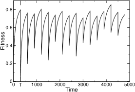
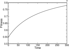
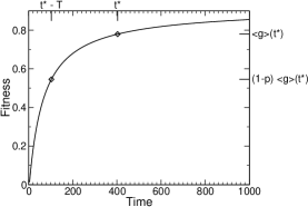
Figure 1: a) Shown is the fitness of a single evolving system with a given modularity as a function of time. Positive fitness means growth of the system. The environment is repeatedly changed each $T=300$ time steps. Shown in b) is the average of these responses during a time $0$ to $T$ after each environmental change, averaged over many environmental changes. Shown in c) is the average response function to $p=1$ environmental changes, $\langle g\rangle(t)$. The response function in b) follows from a master response function curve in c), being the $t^{*}-T$ to $t^{*}$ subset where $\langle g\rangle(t^{*}-T)=(1-p)\langle g\rangle(t^{*})$. Here $p=0.3$ and $T=300$. The present theory applies once the curve in c) has been determined.

The observable $\langle g\rangle(t)$, Fig. 1c, is an input to the theory presented here and comes from a detailed calculation, numerical simulation, or experimental observation of the competitive evolutionary dynamics. The change of environment decreases the fitness by $1-p$ on average Earl and Deem (2004), and the time of evolution in each environment is $T$. These two conditions imply $f_{p,T}(M)=\langle g\rangle(t^{*})$ where $t^{*}$ is defined by

$$\langle g\rangle(t^{*}-T)=(1-p)\langle g\rangle(t^{*})$$ (3)

The function $f_{p,T}(M)$ tells us the average, evolved fitness of the system at the end of each environmental change. This function can be considered to be the fitness when the environmental change is integrated out. This $f_{p,T}(M)$ is the fitness function that goes into Eq. (1).

Evolution of modularity depends on how the response function $f_{p,T}(M)$ of the system varies with the parameters of environmental change, $p$ and $T$. Since systems under stress tend to become more modular, an interpretation is that the average fitness for a modular system is greater than that for a non-modular system, at least for small $T$ or large $p$ where stress is large. This behavior has been observed in a model of systems evolving in a changing environment, when horizontal gene transfer is included Sun and Deem (2007). We have recently proved this canonical behavior for a Moran model of population evolution in a glassy, modular fitness landscape Park et al. (2014). Glassy evolutionary dynamics has been noted a number of times Khatri et al. (2009); Vetsigian et al. (2006). Conversely, at long time, the less modular system should have a higher fitness, because modularity is a constraint on the optima that can be achieved.

In Eq. (1), we here take this function $f(m)$ as input. We assume only that the population averages for large $M$ and small $M$ look like the dashed and solid curves in Fig. 2a. Putting these points together, the quasispecies theory presented here quantitatively describes the emergence of modularity at small $p$ or large $T$, as shown in Figs. 3 and 2b.

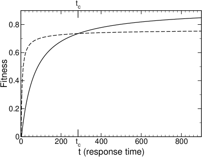
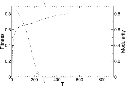
Figure 2: Shown is the fitness of an evolving system. a) The fitness of the non-modular ($\langle g_{0}\rangle$, solid) and block-diagonal ($\langle g_{1}\rangle$, dashed) system are shown, starting from a random initial configuration. These $\langle g_{0}\rangle$ and $\langle g_{1}\rangle$ are inputs to the theory. The modular system is taken to be more fit at short time and less fit at long time. b) The evolved, steady-state fitness of a system predicted by the theory in a changing environment (dot dashed), shown for varying $T$ and $p=1$. The fitness follows the high-modularity curve at rapid environmental changes, small $T$, and the low-modularity curve at slow environmental changes, large $T$. Since $p=1$, the function $f_{p=1,T}(M)=\langle g(M)\rangle(t=T)$. The function $\langle g(M)\rangle$ is here taken for simplicity to be $(1-M)\langle g_{0}\rangle(t)+M\langle g_{1}\rangle(t)$. Note the modularity tends to 1 and the fitness to $\langle g_{1}\rangle$ for rapid environmental change (small $T$), and the modularity tends to 0 and the fitness to $\langle g_{0}\rangle$ for slow environmental change (large $T$). The modularity calculated from theory, Eq. (13), is shown (dotted). Also shown is the theoretical result for small $M$, Eq. (15), to first order in $l/L$ (short dashed). In this example $L=120$, $l=10$, $\mu=0.01$, and $C=5.77$. For these particular $\langle g_{0}\rangle$ and $\langle g_{1}\rangle$, the modularity emerges only for environmental changes that occur on a timescale $T<t_{c}\approx 285$.

IV A Fluctuation Dissipation Theorem

There is a fluctuation dissipation relation for the rate of change of modularity. Multiplying Eq. (1) by $m$ and summing, we find that the rate of change of modularity satisfies

$$\frac{dM}{dt}=L\langle mf(m)\rangle-LM\langle f\rangle-\mu M$$ (4)

This equation is a type of continuous-time Price equation Price (1970). This equation implies a type of useful fluctuation-dissipation theorem. Expanding $f(m)$, we can alternatively write this fluctuation dissipation relation describing the evolution of modularity as

$$\frac{dM}{dt}\approx L\left.\frac{df}{dm}\right|_{M}\langle\sigma^{2}_{M}\rangle-\mu M$$ (5)

Here $M=\langle m\rangle$ is the average modularity of the system, and $\sigma^{2}_{M}=\langle m^{2}\rangle-M^{2}$ is the variance of the modularity, where $m$ is the modularity for any particular system in the population.

V Environmental Change Selects for Modularity

We now derive a relationship between the rate of growth of modularity and the environmental pressure. We investigate the dynamics for small modularity, and we consider a Taylor series expansion of the fitness function: $f(m)=f(0)+m\Delta f+o(m)$. The function $\Delta f$ is time independent, depending on $p$, $T$, and other parameters of the evolution within each system that have been projected out. We investigate the growth of modularity from an initially non-modular state. We consider how the response function depends on $p$. If $p=0$, the environment is not changing, $t^{*}\to\infty$ in the expression of Eq. (3), and the system will stay in the $M=0$ state. This implies $\Delta f=0$ when $p=0$, as otherwise a non-zero modularity would emerge, see Eq. (15) below. For small $p$, the environment is changing only slightly, $t^{*}$ is large, and the system will evolve a small value of $M$. Expanding in a Taylor series for small $p$ and $T\ll t^{*}$, Eq. (3) becomes

$$\frac{p}{T}=\frac{\langle g_{m}^{\prime}\rangle(t_{m}^{*})}{\langle g_{m}\rangle(t_{m}^{*})}\approx\frac{\langle g_{m}^{\prime}\rangle(t_{m}^{*})}{\langle g_{m}\rangle(\infty)}\approx\frac{\langle g_{m}^{\prime}\rangle(t_{m}^{*})}{\langle g_{0}\rangle(\infty)}$$ (6)

where the last two relationships arise because $\langle g_{m}^{\prime}\rangle(t_{m}^{*})$ is small and because $t_{m}^{*}$ is large and $m$ is small. Thus, $\Delta f=\lim_{m\to 0}[f(m)-f(0)]/m=\Delta f(p/T)$. Expanding $\Delta f$ to first order in $p/T$ and taking $m$ small, we find $\Delta f=\alpha p/T$. When $m$ is small, equation (4) becomes

$$M^{\prime}=L\sigma^{2}_{M}\Delta f-\mu M$$ (7)

Using the result above for $\Delta f$, we find $M^{\prime}\approx\alpha L\sigma^{2}_{M}p/T$, leaving out the small term proportional to $M$ in Eq.  (7). We, thus, find

$$p_{\rm E}\approx\frac{1}{R}\frac{dM}{dt}$$ (8)

where $p_{\rm E}=p/T$ is the environmental pressure, and $R=\alpha L\sigma_{M}^{2}$. In this equation, $R\propto\langle\sigma_{M}^{2}\rangle$, which as experimentalists have anticipated is related to replicate variability in experiments Cooper and Lenski (2010).

This Eq. (8) follows from the fluctuation dissipation relation in Eq. (4) and the response function of the modular system being greater than that of the non-modular system at short time. Equation (8) may be interpreted as a Taylor series expansion of $dM/dt$ in allowed combinations of $p$ and $1/T$. Alternatively, Eq. (8) may be interpreted as the linear response of the modularity to the environmental pressure. The coefficient $R$ is a measure of ruggedness of the evolutionary landscape within each system. This ruggedness slows down the evolutionary dynamics, and the selection for an effective response function provided by a changing environment implicitly selects for modularity when horizontal gene transfer is active Sun and Deem (2007). Here, we are able to show that $R$ is proportional to the variance of the modularity, which is expected to be related to the ruggedness of the landscape. It is the ruggeddness of the landscape that leads to non-trivial replicate variability.

For what forms of $\langle g_{m}\rangle(t)$ will the $\Delta f(p/T)$ function be analytic in $p/T$? We first consider an exponential convergence of the fitness function: $\langle g_{m}\rangle(t)=g(\infty)-a_{m}\exp(-\beta_{m}t)$, where we have left out the $m$ depencence of $g(\infty)$ because we expect it to be higher order than linear in $m$. Eq. (6) becomes $pg(\infty)/T=a_{m}\beta_{m}\exp(-\beta_{m}t^{*}_{m})$, and we find $f_{p,T}(m)=\langle g_{m}\rangle(t^{*}_{m})=g(\infty)-g(\infty)p/(T\beta_{m})$. We thus find $m\Delta f=g(\infty)(p/T)(1/\beta_{0}-1/\beta_{m})$, which is positive because we expect the modular system to converge faster, $\beta_{m}>\beta_{0}$. Thus, we find Eq. (8), with $\alpha=-g(\infty)d\beta_{m}^{-1}/dm|_{m=0}$. Conversely, for a power law decay $\langle g_{m}\rangle(t)=g(\infty)-a_{m}t^{-\beta}$, we find the fitness to be non-linear in $p/T$: $f_{p,T}(m)=g(\infty)-a_{m}[(pg(\infty)/(Ta_{m}\beta)]^{\beta/(\beta+1)}$. In this case, Eq. (8) is modified to be $p_{\rm E}^{\beta/(\beta+1)}$ on the left hand side, with $\alpha=-[g(\infty)/\beta]^{\beta/(\beta+1)}da_{m}^{1/(\beta+1)}/dm|_{m=0}$. Finally, for a logarithmic decay Park et al. (2014) $\langle g_{m}\rangle(t)=g(\infty)-a_{m}\ln^{-2/\nu}(t/t^{0}_{m})$, we find the fitness to be non-analytic in $p/T$, since $(p/T)t^{*}_{m}g(\infty)=(2/\nu)a_{m}\ln^{-2/\nu-1}(t^{*}_{m}/t^{0}_{m})$. This equation can be solved in terms of powers of the product logarithm, or Lambert $W_{0}$ function. Performing an asymptotic analysis for small $p/T$, we find $f_{p,T}(m)\sim g(\infty)-a_{m}\ln^{-2/\nu}(T/p)$. In this case, Eq. (8) is modified to be $1/(\ln^{2}p_{\rm E})^{1/\nu}$ on the left hand side, with $\alpha=-da_{m}/dm|_{m=0}$.

Equation (8) is a description of how the evolvability of the system depends on the environmental change. That is, $dM/dt$ is a measure of the evolvability of the system, with larger values indicating a greater rate of change of the measurable order parameter $M$. This measure of evolvability is greater for greater environmental pressures, $p_{\rm E}$. The drive for spontaneous emergence of modularity, large $dM/dt$, is also greater for landscapes that are more rugged, i.e. larger $R$, which can be estimated from variability of replicate experiments.

Equation (8) says that an increase of environmental pressure should lead to the evolution of systems with increased modularity. A study of 117 species of bacteria showed that the modularity of the bacteria’s metabolic networks increased monotonically with variability of the environment in which the bacteria lived Parter et al. (2007). Metabolic networks of pathogens alternating between hosts were found to be more modular than those of single-host pathogens Kreimer et al. (2008).

VI Steady-State Values of Modularity in One Environment

VI.1 Field Theory for the Dynamics of Modularity

Here we rewrite the dynamical equations of quasispecies theory in the language of field theory. We solve the field theory in the limit of large system sizes to determine the steady-state modularity that emerges at long time. The theory is distinct from traditional quasispecies theory because the replication rate depends on the modularity rather than the Hamming distance from a wild-type strain. Nonetheless, we will show that the theory can still be solved exactly in the limit of a large system size.

For large values of $L$, for which the changes in $M$ are nearly continuous, we here determine the average fitness implied by Eq. (1) at long time by techniques borrowed from quantum field theory Peliti (2002); Park and Deem (2006). We write the dynamical equations in Eq. (1) in terms of raising and lowering operators. We then use coherent states to write this second quantization in terms of a Bosonic field theory, with fields $z^{*}_{ij}(t),z_{ij}(t)$ representing density at $\Delta_{ij}(t)$ at time $t$. The action of this field theory is

$$S[\{z\},\{z^{*}\}] = \int_{0}^{t_{f}}\sum_{ij}z_{ij}^{*}(t)\partial_{t}z_{ij}(t)dt+\sum_{ij}\left[z_{ij}^{*}(0)z_{ij}(0)-z_{ij}(t_{f})\right]+LC$$ (9)

$$-\frac{C_{1}}{L}\sum_{ij}^{\rm in}z_{ij}^{*}(0)-\frac{C_{0}}{L}\sum_{ij}^{\rm out}z_{ij}^{*}(0)$$

$$-L\int_{0}^{t_{f}}f\left[\frac{1}{LC}\left(\sum_{ij}^{\rm in}z_{ij}^{*}(t)z_{ij}(t)-\frac{1}{L/l-1}\sum_{ij}^{\rm out}z_{ij}^{*}(t)z_{ij}(t)\right)\right]dt$$

$$-\frac{\mu}{L^{2}}\int_{0}^{t_{f}}\sum_{ij}\sum_{mn}[z_{mn}^{*}(t)-z_{ij}^{*}(t)]z_{ij}(t)dt$$

Note that the fitness depends on the modularity of the connection matrices of each state at each point in time in Eq. (9), just as it did in Eq. (1). Also note that Eqs. (1) and (9) are exact for arbitrary, non-linear fitness functions $f(m)$. Here “in” means in the $l\times l$ block diagonals and “out” means outside these block diagonals. The quadratic terms can be integrated out (see Appendix B) Park and Deem (2006), and we are left with an action expressed in terms of a modularity field, $\xi$, and its conjugate, $\bar{\xi}$:

$$S = L\int_{0}^{t_{f}}[C\bar{\xi}(t)\xi(t)-f(\xi(t))]dt-LC\ln Q$$ (10)

where the determinant is $Q=[lC_{1}(t_{f})+(L-l)C_{0}(t_{f})]/(LC)$, where the vector ${\bf C}(t)=(C_{1}(t),C_{0}(t))$ satisfies

$$d{\bf C}/dt=A(t){\bf C}(t)$$ (11)

where

$$A(t)=\left(\begin{array}[]{cc}-\mu(L-l)/L+\bar{\xi}(t)&\mu(L-l)/L\\ \mu l/L&-\mu l/L-\bar{\xi}(t)l/(L-l)\end{array}\right)$$ (12)

and ${\bf C}(0)=(C_{1},C_{0})$.

VI.2 The Steady-State, Average Value of Modularity

The average modularity follows a dynamical trajectory away from an initial state to a final steady state value. For large $L$, this action becomes large, and a saddle point calculation can be used (see Appendix C). The remarkable result from this derivation is that the modularity which emerges at long time obeys a principle of least action:

$$f_{\rm pop}=\max_{\xi}\left\{f(\xi)-\mu C[(L-l)l/L^{2}][2+(L/l-2)\xi-2\sqrt{(1-\xi)(1+(L/l-1)\xi)}]\right\}$$ (13)

The variance of the modularity is small, ${\cal O}(1/L)$, and the modularity is determined by the solution of the implicit equation

$$f(M)=f_{\rm pop}$$ (14)

Here $f_{\rm pop}$ is the mean population fitness, i.e. Eq. (2) with $t\to\infty$. Thus, a principle of least action gives the evolved modularity at steady state. Coexistence of populations with different modularity, i.e. bimodality in the distribution of modularity, is possible if the $f(m)$ function is discontinuous Park and Deem (2007).

VI.3 Phase Diagrams for The Emergence of Modularity

While Eq. (13) is a general result, we can proceed further in the limit that evolved modularities are small. Expanding for small $M$, we find

$$\xi_{\rm max} \sim \frac{2l\left[df/dM|_{M=0}\right]}{\mu C(L-l)-2l\left[d^{2}f/dM^{2}|_{M=0}\right]}$$

$$f_{\rm pop} \sim \frac{l\left[df/dM|_{M=0}\right]^{2}}{\mu C(L-l)-2l\left[d^{2}f/dM^{2}|_{M=0}\right]}+f(0)$$

$$M \sim \frac{l\left[df/dM|_{M=0}\right]}{\mu C(L-l)-2l\left[d^{2}f/dM^{2}|_{M=0}\right]}$$ (15)

Thus, as long as a modular system has a higher fitness, $df/dM>0$, modularity will spontaneously emerge, $M>0$, for large enough system sizes, $L$. Note also when $M$ is small, that the steady state modularity calculated exactly from Eq. (13) is in agreement with the small $M$ result in Eq. (15), as shown in Fig. 2b. Note that for large $L/l$, Eq. (7) combined with Eq. (15) implies that at steady state $\sigma^{2}_{M_{\infty}}=l/[L(L-l)C]$.

For fitness functions for which $df/dM|_{M=0}=0$, more analysis is required. For example, if $f(M)=kM^{2}/2$, there is a phase transition at $\mu^{*}$: For $\mu<\mu^{*}$ modularity emerges, whereas for $\mu>\mu^{*}$ the population remains in the non-modular phase. This phase transition is analogous to the error catastrophe found in traditional quasispecies theory. Phase diagrams for a number of fitness functions are shown in Fig. 3.

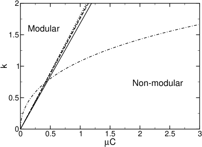
Figure 3: The phase diagram for emergence of modularity. Below a critical mutation rate, modularity spontaneously emerges. Results are shown for $f(M)=kM^{2}/2$ (solid), $f(M)=kM^{3}/2$ (long-dashed), $f(M)=kM^{4}/2$ (short-dashed), $f(M)=kM^{10}/2$ (dotted), and $f(M)=e^{kM}-kM-1$ (dot-dashed). Results here are shown for $l=10,L=120$.

VII Using Quasispecies Theory to Extrapolate Simulation Data on Spontaneous Emergence of Modularity

We use Eq. (1) to analyze $M(t)$ data on spontaneous emergence of modularity in a simulation of an evolving protein network Sun and Deem (2007) to deduce $df/dm$ and to derive $f(M)$ by integration. For this system, we know the mutation rate, as two of the connections change per time step in the upper half of the connection matrix, and so we can use Eq. (1) at short time to determine $df/dm$. Alternatively we can determine $df/dm$ if we know the variance of the modularity and $M(t)$, c.f. Eq. (5). We assume $f(M)$ is quadratic, and integrate the $df/dm$ to determine the $f(M)$. There are $N_{D}=346$ total connections in the upper half of the connection matrix and $N_{0}=22$ connections in the upper half of the connection matrix when $M=0$ for the parameters of Sun and Deem (2007). Thus, we take $C=346\times 2/L=5.77$ and $\mu=2/346$. When $M=0$, the population was prepared by four discrete time iterations of the mutation step, from a single initial configuration Sun and Deem (2007). We find $f(M)\sim 1.4M$ reproduces the data at small $M$. For the initial condition of $M=0.38$, the configurations were taken from an ensemble Sun and Deem (2007), which we take to satisfy Eq. (1). We find $f(M)=1.4M-1.31M^{2}$ approximately reproduces the data, as shown in Fig. 4. Equation (13) predicts a steady-state value of $M=0.45$, toward which the computationally costly simulations appear to be heading.

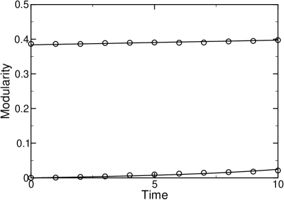
Figure 4: Shown is modularity versus time for a population that exhibits spontaneous emergence of modularity. The curves are from theory, Eq. (1), and the data (circles) are from Sun and Deem (2007). Two different initial conditions are shown, $M(0)=0$ and $M(0)=0.38$. In this example the derived underlying fitness function is $f(M)=1.4M-1.31M^{2}$, the mutation rate is $\mu=2/346$, and the average number of connections is $C=346\times 2/L=5.77$.

VIII Conclusion

The examples of environmental stress leading to modularity, ranging from metabolic networks of bacteria in different physical environment to simulations of emergence of protein secondary structure, can be quantified by quasispecies theory. The approximate relation $Rp_{\rm E}=dM/dt$ relates rate of growth of modularity to the ruggedness of the fitness landscape, $R$, and environmental pressure, $p_{\rm E}$, for small values of modularity. The present theory should allow the analysis of complex, evolving populations to go beyond a demonstration of the existence of modularity to a quantitative analysis of the dynamics of modularity. That is, the theory presented here should allow the determination of the $f(M)$ function for these evolving populations, by using the predictions to determine the $f(M)$ that best matches observation. Knowing the $f(M)$ and $\mu$ that fundamentally characterize a population would then allow for out-of-sample predictions of dynamical modularity.

IX Appendix A

We here derive Eq. (1). The rate to increase modularity for a matrix with modularity $m$ is $r_{\rm up}=\mu n_{\rm out}(L/l)l^{2}/L^{2}$. Recall we are in the dilute limit: $C$ is finite, and $L$ is large. Thus, collisions between entries in the connection matrix can be ignored. The rate to decrease modularity for a matrix with modularity $m$ is $r_{\rm down}=\mu n_{\rm in}L(L-l)/L^{2}$. Here the number of connections inside the $l\times l$ blocks is given by $n_{\rm in}$ and the number of connections outside the $l\times l$ blocks is given by $n_{\rm out}$. We have the constraint $n_{\rm in}+n_{\rm out}=CL$. We also have by the definition of modularity $m=[n_{\rm in}/l-n_{\rm out}/(L-l)]l/(CL)$, which shows modularity changes by discrete increments of $\pm 1/[C(L-l)]$. Thus, we find $r_{\rm up}(m)=\mu Cl(L-l)(1-m)/L$ and $r_{\rm down}(m)=\mu C(L-l)(Lm-lm+l)/L$. For non-zero modularity, to avoid collisions in the $\Delta$ matrix, we further require $\langle n_{\rm in}\rangle\ll lL$, i.e. $C(l-lM+LM)\ll lL$. Alternatively, if this constraint is not satisfied, we can view Eq. (1) as a generalization to the case of integer occupation numbers of the $\Delta$ matrix with certain biased hopping probabilities, $r_{\rm up}(m)$ and $r_{\rm down}(m)$, given above. The rate of change of $P_{m}(t)$ due to replication is $L[f(m)-\langle f\rangle]P_{m}(t)$, where the second term ensures conservation of probability, $\sum_{m}P_{m}(t)=1\ \forall\ t$. This is the first term on the right hand side in Eq. (1). The rate of increasing $P_{m}(t)$ due to an increase of modularity from $m-1/[C(L-l)]$ to $m$ is $r_{\rm up}[m-1/(C(L-l))]P_{m-1/[C(L-l)]}(t)$, which is the first $\mu$-dependent term in Eq. (1). The rate of increasing $P_{m}(t)$ due to a decrease of modularity from $m+1/[C(L-l)]$ to $m$ is $r_{\rm down}[m+1/(C(L-l))]P_{m+1/[C(L-l)]}(t)$, which is the second $\mu$-dependent term in Eq. (1). The rate of decreasing $P_{m}(t)$ due to modularity changing from $m$ to $m\pm 1/[C(L-l)]$ is $[r_{\rm up}(m)+r_{\rm down}(m)]P_{m}(t)$, which is the third $\mu$-dependent term in Eq. (1). Thus, we have derived Eq. (1).

X Appendix B

We here calculate the determinant that comes from integrating out the $z^{*}_{ij}$ and $z_{ij}$ fields in Eq. (9). The probability of connections inside and outside the blocks have been taken initially to be Poisson in Eq. (9), with average probability of a connection per site to be $C_{1}/L$ inside the blocks and $C_{0}/L$ outside the blocks. The overall average number of connections per row is $C=C_{0}+(C_{1}-C_{0})l/L$. We here project the number of connections onto the constraint that there are $LC$ total connections. As in Park and Deem (2006), this constraint is enforced with a projection operator that leads to twisted boundary conditions. A modularity field $\xi$ and conjugate field $\bar{\xi}$ are defined, with $\xi(t)$ as the argument of the fitness function in Eq. (9). We use a trotter factorization and define $\epsilon=t_{f}/M$ and will take the limit $M\to\infty$. We define $\delta=1$ if $\lfloor i/l\rfloor=\lfloor j/l\rfloor$ and zero otherwise. The partition function becomes

$$\cal Z = \int[{\cal D}\bar{\xi}{\cal D}\xi]e^{-\epsilon LC\sum_{k=1}^{M}\bar{\xi}(k)\xi(k)+\epsilon L\sum_{k=1}^{M}f[\xi(k)]}$$ (16)

$$\times\int_{0}^{2\pi}\frac{d\eta}{2\pi}e^{-i\eta-LC}[{\cal D}z^{*}{\cal D}z]e^{-\sum_{k=0}^{M}\sum_{ij}z^{*}_{ij}(k)z_{ij}(k)+\sum_{ij}z_{ij}(M)}$$

$$\times e^{\sum_{k=1}^{M}\sum_{ij}\left[z^{*}_{ij}(k)+(\epsilon\mu/L^{2})\sum_{mn}(z^{*}_{mn}(k)-z^{*}_{ij}(k))+\epsilon\bar{\xi}(k)(L\delta-l)/(L-l)z^{*}_{ij}(k)\right]z_{ij}(k-1)}$$

$$\times e^{(C_{1}(0)/L)e^{i\eta/(LC)}\sum_{ij}^{\rm in}z^{*}_{ij}(0)+(C_{0}(0)/L)e^{i\eta/(LC)}\sum_{ij}^{\rm out}z^{*}_{ij}(0)}$$

Integrating out $z^{*}_{ij}(0)$ and $z_{ij}(0)$, the action remains the same except the start on sums over $k$ are incremented by one, and the terms $C_{1}(0)z^{*}(0)$ and $C_{0}(0)z^{*}(0)$ become $C_{1}(1)z^{*}(1)$ and $C_{0}(1)z^{*}(1)$ with

$$C_{1}(1) = C_{1}(0)\left[1-\epsilon\mu\left(1-\frac{l}{L}\right)+\epsilon\bar{\xi}(1)\right]+C_{0}(0)\epsilon\mu\left(1-\frac{l}{L}\right)$$

$$C_{0}(1) = C_{0}(0)\left[1-\epsilon\mu\frac{l}{L}-\epsilon\bar{\xi}(1)\frac{l}{L-l}\right]+C_{1}(0)\epsilon\mu\frac{l}{L}$$ (17)

Iterating the process of integrating out the $z^{*}(k)$ and $z(k)$, we find that the vector ${\bf C}(t)=(C_{1}(t),C_{0}(t))$ renormalizes according to Eq. (11). Finally, integrating out $z^{*}(M)$ and $z(M)$, we find the final contribution to the partition function is

$$\cal Z = \int[{\cal D}\bar{\xi}{\cal D}\xi]e^{-\epsilon LC\sum_{k=1}^{M}\bar{\xi}(k)\xi(k)+\epsilon L\sum_{k=1}^{M}f[\xi(k)]}$$ (18)

$$\times\int_{0}^{2\pi}\frac{d\eta}{2\pi}e^{-i\eta-LC}e^{[lC_{1}(M)+(L-l)C_{0}(M)]e^{i\eta/(LC)}}$$

Performing the final integration over $\eta$, we find the final expression for the partition function to be

$$\cal Z = \int[{\cal D}\bar{\xi}{\cal D}\xi]e^{-\epsilon LC\sum_{k=1}^{M}\bar{\xi}(k)\xi(k)+\epsilon L\sum_{k=1}^{M}f[\xi(k)]}\left[\frac{lC_{1}(M)+(L-l)C_{0}(M)}{LC}\right]^{LC}$$ (19)

Thus, the action in Eq. (10) is derived.

XI Appendix C

Here we calculate the saddle-point solution to the action (10) at large time. For large $L$, this saddle point solution is exact. For large $t_{f}$, Eq. (10) becomes

$$S=Lt_{f}[C\bar{\xi}\xi-f(\xi)]-LC\ln Q$$ (20)

where

$$Q=Tr\left[e^{t_{f}A}\left(\begin{array}[]{c}C_{1}(0)/C\\ C_{0}(0)/C\end{array}\right)\left(\frac{l}{L},\frac{L-l}{L}\right)\right]$$ (21)

The larger eigenvalue of $A$ is given by

$$\lambda_{+}=-\frac{1}{2}\left(\mu-\frac{L-2l}{L-l}\bar{\xi}\right)+\frac{1}{2}\left[\left(\mu-\frac{L-2l}{L-l}\bar{\xi}\right)^{2}+\frac{4l\bar{\xi}^{2}}{L-l}\right]^{1/2}$$ (22)

Thus, the action tends to

$$-S\sim Lt_{f}[-C\bar{\xi}\xi+f(\xi)]+LCt_{f}\lambda_{+}$$ (23)

Maximizing this over $\bar{\xi}$, we find

$$-S/(Lt_{f})\sim f(\xi)-\mu C[(L-l)l/L^{2}][2+(L/l-2)\xi-2\sqrt{(1-\xi)(1+(L/l-1)\xi)]}$$ (24)

Maximizing over $\xi$ gives Eq. (13). Using that the partition function $\cal Z$ grows at long time as $\exp(Lf_{\rm pop}t_{f})$ Park and Deem (2006), we find Eq. (14).

References

- Waddington (1942) C. H. Waddington, Nature 150, 563 (1942).
- Simon (1962) H. A. Simon, Proc. Amer. Phil. Soc. 106, 467 (1962).
- Hartwell et al. (1999) L. H. Hartwell, J. J. Hopfield, S. Leibler, and A. W. Murray, Nature 402, C47 (1999).
- Ravasz et al. (2002) E. Ravasz, A. L. Somera, D. A. Mongru, Z. N. Oltvai, and A.-L. Barabási, Science 297, 1551 (2002), URL http://www.sciencemag.org/cgi/content/abstract/297/5586/1551.
- Callahan et al. (2009) B. Callahan, M. Thattai, and B. I. Shraiman, Proc. Natl. Acad. Sci. USA 106, 19410 (2009), URL http://www.pnas.org/cgi/content/abstract/106/46/19410.
- da Silva et al. (2008) M. R. da Silva, H. Ma, and A.-P. Zeng, Pr. Inst. Electr. Elect. 96, 1411 (2008), URL http://ieeexplore.ieee.org/xpl/freeabs_all.jsp?arnumber=4567%408.
- Spirin and Mirny (2003) V. Spirin and L. A. Mirny, Proc. Natl. Acad. Sci. USA 100, 12123 (2003), URL http://www.pnas.org/cgi/content/abstract/100/21/12123.
- Gavin et al. (2006) A.-C. Gavin, P. Aloy, P. Grandi, R. Krause, M. Boesche, M. Marzioch, C. Rau, L. J. Jensen, S. Bastuck, B. Dümpelfeld, et al., Nature 440, 631 (2006), URL http://www.ncbi.nlm.nih.gov/pubmed/16429126.
- von Mering et al. (2003) C. von Mering, E. M. Zdobnov, S. Tsoka, F. D. Ciccarelli, J. B. Pereira-Leal, C. A. Ouzounis, and P. Bork, Proc. Natl. Acad. Sci. USA 100, 15428 (2003), URL http://www.pnas.org/cgi/content/abstract/100/26/15428.
- Krause et al. (2003) A. E. Krause, K. A. Frank, D. M. Mason, R. E. Ulanowicz, and W. W. Taylor, Nature 426, 282 (2003), URL http://www.ncbi.nlm.nih.gov/pubmed/14628050.
- Raff and Raff (2000) E. C. Raff and R. A. Raff, Evol. Dev. 2, 235 (2000), URL http://www3.interscience.wiley.com/journal/119052048/abstract%.
- Wagner (1996) G. P. Wagner, Integr. Comp. Biol. 36, 36 (1996), URL http://icb.oxfordjournals.org/cgi/content/abstract/36/1/36.
- Klingenberg (2008) C. P. Klingenberg, Annu. Rev. Ecol. Evol. S. 39, 115 (2008), URL http://search.ebscohost.com/login.aspx?direct=true&db=a9h&A%N=35967311.
- Meunier et al. (2009) D. Meunier, S. Achard, A. Morcom, and E. Bullmore, NeuroImage 44, 715 (2009), URL http://www.ncbi.nlm.nih.gov/pubmed/19027073.
- Chavez et al. (2010) M. Chavez, M. Valencia, V. Navarro, V. Latora, and J. Martinerie, Phys. Rev. Lett. 104, 118701 (2010), URL http://prl.aps.org/abstract/PRL/v104/i11/e118701.
- Mihalik and Csermely (2011) A. Mihalik and P. Csermely, PLoS Comput. Biol. 7, e1002187 (2011).
- He et al. (2009) J. He, J. Sun, and M. W. Deem, Phys. Rev. E 79, 031907 (2009).
- Lorenz et al. (2011) D. M. Lorenz, A. Jeng, and M. W. Deem, Phys. Life Rev. 8, 129 (2011).
- Rietkerk et al. (2004) M. Rietkerk, S. C. Dekker, P. C. de Ruiter, and J. van de Koppel, Science 305, 1926 (2004).
- Tinker et al. (2008) M. T. Tinker, G. Bentall, and J. A. Estes, Proc. Natl. Acad. Sci. USA 105, 560 (2008).
- Saavedra et al. (2011) S. Saavedra, K. Hagerty, and B. Uzzi, Proc. Natl. Acad. Sci. USA 108, 5296 (2011).
- Estrada and Hatano (2010) E. Estrada and N. Hatano, in Econophysics approaches to large-scale business data and financial crisis, edited by M. Takayasu, T. Watanabe, and H. Takayasu (Springer, 2010), pp. 271–288.
- He and Deem (2010) J. He and M. W. Deem, Phys. Rev. Lett. 105, 198701 (2010), URL http://prl.aps.org/abstract/PRL/v105/i19/e198701.
- Haldane and May (2011) A. G. Haldane and R. M. May, Nature 469, 351 (2011).
- Hallinan (2004) J. S. Hallinan, Biosystems 74, 51 (2004), URL http://dx.doi.org/10.1016/j.biosystems.2004.02.004.
- Rainey and Cooper (2004) P. B. Rainey and T. F. Cooper, Res. Microbiol 155, 370 (2004), URL http://dx.doi.org/10.1016/j.resmic.2004.01.011.
- Sun and Deem (2007) J. Sun and M. W. Deem, Phys. Rev. Lett. 99, 228107 (2007).
- Lipson et al. (2002) H. Lipson, J. B. Pollack, and N. P. Suh, Evolution 56, 1549 (2002).
- Kashtan and Alon (2005) N. Kashtan and U. Alon, Proc. Natl. Acad. Sci. USA 102, 13773 (2005).
- Kashtan et al. (2007) N. Kashtan, E. Noor, and U. Alon, Proc. Natl. Acad. Sci. USA 104, 13711 (2007).
- Eigen (1971) M. Eigen, Naturwissenschaften 58, 465 (1971).
- Crow and Kimura (1970) J. F. Crow and M. Kimura, An Introduction to Population Genetics Theory (Harper and Row, New York, 1970).
- Jain and Krug (2005) K. Jain and J. Krug, in Structural approaches to sequence evolution: Molecules, networks and populations, edited by H. R. U. Bastolla, M. Porto and M. Vendruscolo (Springer Verlag, Berlin, 2005), pp. 299–339, q-bio.PE/0508008.
- Leuthäusser (1986) I. Leuthäusser, J. Chem. Phys 84, 1884 (1986).
- Tarazona (1992) P. Tarazona, Phys. Rev. A 45, 6038 (1992).
- Baake et al. (1997) E. Baake, M. Baake, and H. Wagner, Phys. Rev. Lett. 78, 559 (1997), 79, 1782.
- Baake et al. (1998) E. Baake, M. Baake, and H. Wagner, Phys. Rev. E 57, 1191 (1998).
- Saakian and Hu (2004) D. B. Saakian and C.-K. Hu, Phys. Rev. E 69, 021913 (2004).
- Peliti (2002) L. Peliti, Europhys. Lett. 57, 745 (2002).
- Saakian et al. (2006) D. B. Saakian, E. Munoz, C.-K. Hu, and M. W. Deem, Phys. Rev. E 73, 041913 (2006).
- Park and Deem (2006) J.-M. Park and M. W. Deem, J. Stat. Phys. 125, 975 (2006).
- Saakian et al. (2008) D. B. Saakian, O. Rozanova, and A. Akmetzhanov, Phys. Rev. E 78, 041908 (2008).
- Munoz et al. (2009) E. T. Munoz, J.-M. Park, and M. W. Deem, J. Stat. Phys. 135, 429 (2009).
- Cohen et al. (2005) E. Cohen, D. A. Kessler, and H. Levine, Phys. Rev. Lett. 94, 098102 (2005).
- Park and Deem (2007) J.-M. Park and M. W. Deem, Phys. Rev. Lett. 98, 058101 (2007).
- Munoz et al. (2008) E. T. Munoz, J.-M. Park, and M. W. Deem, Phys. Rev. E 78, 061921 (2008).
- Park et al. (2010) J.-M. Park, E. Muñoz, and M. W. Deem, Phys. Rev. E 81, 011902 (2010).
- Lorenz et al. (2013) D. M. Lorenz, J.-M. Park, and M. W. Deem, Phys. Rev. E 87, 022704 (2013).
- Deem and Lee (2003) M. W. Deem and H.-Y. Lee, Phys. Rev. Lett. 91, 068101 (2003).
- Sun et al. (2005) J. Sun, D. J. Earl, and M. W. Deem, Phys. Rev. Lett. 95, 148104 (2005).
- Munoz and Deem (2004) E. T. Munoz and M. W. Deem, Vaccine 23, 1142 (2004).
- Gupta et al. (2006) V. Gupta, D. J. Earl, and M. W. Deem, Vaccine 24, 3881 (2006), URL http://dx.doi.org/10.1016/j.vaccine.2006.01.010.
- Zhou and Deem (2006) H. Zhou and M. W. Deem, Vaccine 24, 2451 (2006).
- Earl and Deem (2004) D. J. Earl and M. W. Deem, Proc. Natl. Acad. Sci. USA 101, 11531 (2004).
- Park et al. (2014) J. Park, M. Chen, D. Wang, and M. W. Deem (2014), submitted.
- Khatri et al. (2009) B. S. Khatri, T. C. McLeish, and R. P. Sear, Proc. Natl. Acad. Sci. USA 1006, 9564 (2009).
- Vetsigian et al. (2006) K. Vetsigian, C. Woese, and N. Goldenfeld, Proc. Natl. Acad. Sci. USA 103, 10696 (2006).
- Price (1970) G. R. Price, Nature 227, 520 (1970).
- Cooper and Lenski (2010) T. F. Cooper and R. E. Lenski, BMC Evol. Biol. 10, 1e11 (2010).
- Parter et al. (2007) M. Parter, N. Kashtan, and U. Alon, BMC Evol. Biol. 7, 169 (2007).
- Kreimer et al. (2008) A. Kreimer, E. Borenstein, U. Gophna, and E. Ruppin, Proc. Natl. Acad. Sci. USA 105, 6976 (2008).