Theano: new features and speed improvements

Abstract

Theano is a linear algebra compiler that optimizes a user’s symbolically-specified mathematical computations to produce efficient low-level implementations. In this paper, we present new features and efficiency improvements to Theano, and benchmarks demonstrating Theano’s performance relative to Torch7, a recently introduced machine learning library, and to RNNLM, a C++ library targeted at recurrent neural networks.

1 Introduction

Theano was introduced to the machine learning community by Bergstra et al. (2010) as a CPU and GPU mathematical compiler, demonstrating how it can be used to symbolically define mathematical functions, automatically derive gradient expressions, and compile these expressions into executable functions that outperform implementations using other existing tools. Bergstra et al. (2011) then demonstrated how Theano could be used to implement Deep Learning models.

In Section 2, we will briefly expose the main goals and features of Theano. Section 3 will present some of the new features available and measures taken to speed up Theano’s implementations. Section 4 compares Theano’s performance with that of Torch7 (Collobert et al., 2011) on neural network benchmarks, and RNNLM (Mikolov et al., 2011) on recurrent neural network benchmarks.

2 Main features of Theano

Here we briefly summarize Theano’s main features and advantages for machine learning tasks. Bergstra et al. (2010, 2011), as well as Theano’s website have more in-depth descriptions and examples.

2.1 Symbolic Mathematical Expressions

Theano includes powerful tools for manipulating and optimizing graphs representing symbolic mathematical expressions. In particular, Theano’s optimization constructs can eliminate duplicate or unnecessary computations (e.g., replacing $x-x$ by $0$, obviating the need to compute $x$ in the first place), increase numerical stability (e.g., by substituting stable implementations of $\log(1+x)$ when $x$ is tiny, or $\log(\operatorname{sigmoid}(x))$), or increase speed (e.g., by using loop fusion to apply a sequence of scalar operations to all elements of an array in a single pass over the data).

This graph representation also enables symbolic differentiation of mathematical expressions, which allows users to quickly prototype complex machine learning models fit by gradient descent without manually deriving the gradient, decreasing the amount of code necessary and eliminating several sources of practitioner error. Theano now supports forward-mode differentiation via the R-operator (see Section 3.2) as well as regular gradient backpropagation. Theano is even able to derive symbolic gradients through loops specified via the Scan operator (see Section 3.1).

2.2 Fast to write and to execute

Theano’s dependency on NumPy and SciPy (Jones et al., 2001) makes it easy to add an implementation for a mathematical operation, leveraging the effort of their developers, and it is always possible to add a more optimized version that will then be transparently substituted where applicable. For instance, Theano defines operations on sparse matrices using SciPy’s sparse matrix types to hold values. Some of these operations simply call SciPy’s functions, other are reimplemented in C++, using BLAS routines for speed.

2.3 Parallelism on the GPU

Theano uses CUDA to define a class of $n$-dimensional (dense) arrays located in GPU memory with Python bindings. Theano also includes CUDA code generators for fast implementations of mathematical operations. Most of these operations are currently limited to dense arrays of single-precision floating-point numbers.

2.4 Stability and community support

Theano’s development team has increased its commitment to code quality and correctness as Theano usage begins to spread across university and industry laboratories: a full test suite runs every night, with a shorter version running for every pull request, and the project makes regular stable releases. There is also a growing community of users who ask and answer questions every day on the project’s mailing lists.

3 New features in Theano

This section presents features of Theano that have been recently developed or improved. Some of these are entirely novel and extend the scenarios in which Theano can be used (notably, Scan and the R operator); others aim at improving performance, notably reducing the time not spent in actual computation (such as Python interpreter overhead), and improving parallelism on CPU and GPU.

3.1 Scan: Symbolic Loop in Theano

Theano offers the ability to define symbolic loops through use of the Scan Op, a feature useful for working with recurrent models such as recurrent neural networks, or for implementing more complex optimization algorithms such as linear conjugate gradient.

Scan surmounts the practical difficulties surrounding other approaches to loop-based computation with Theano. Using Theano’s symbolically-defined implementations within a Python loop prevents symbolic differentiation through the iterative process, and prevents certain graph optimizations from being applied. Completely unrolling the loop into a symbolic chain often leads to an unmanageably large graph and does not allow for “while”-style loops with a variable number of iterations.

The Scan operator is designed to address all of these issues by abstracting the entire loop into a single node in the graph, a node that communicates with a second symbolic graph representing computations inside the loop. Without going into copious detail, we present a list of the advantages of our strategy and refer to section 4.3 where we empirically demonstrate some of these advantages. Tutorials available from the Theano website offer a detailed description of the required syntax as well as example code.

1. Scan allows for efficient computation of gradients and implicit “vector-Jacobian” products. The specific algorithm used is backpropagation through time Rumelhart et al. (1986), which optimizes for speed but not memory consumption.

2. Scan allows for efficient evaluation of the R-operator (see Pearlmutter (1994)), required for computing quantities such as the Gauss-Newton approximation of Hessian-vector products.

3. The number of iterations performed by Scan can itself be expressed as a symbolic variable (for example, the length of some input sequence) or a symbolically specified condition, in which case Scan behaves as a “do while” statement. If the number of steps is fixed and equal to 1, the Scan node is “unrolled” into the outer graph for better performance.

4. Any loop implemented with Scan can be transparently transferred to a GPU (if the computation at each iteration can itself be performed on the GPU).

5. The body of Scan (which involves computing indices of where to pick input slices and where to put the output of each iteration) is implemented with Cython to minimize the overhead introduced by necessary bookkeeping between each iteration step.

6. Whenever possible, Scan detects the amount of memory necessary to carry out an operation: it examines intermediate results and makes an informed decision as to whether such results are needed in subsequent iterations in order to partially optimize memory reuse. This decision is taken at compilation time.

7. Loops represented as different Scan instances are merged (given that certain necessary conditions are respected, e.g., both loops perform the same number of steps). This aids not only in reducing the overhead introduced by each instance of Scan, but also helps optimize the computation performed at each iteration of both loops, e.g. certain intermediate quantities may be useful to the body of each individual loop, and will be computed only once in the merged instance.

8. Finally, whenever a computation inside the loop body could be performed outside the loop, Scan moves said computation in the main graph. For example element-wise operations are moved outside, where, given that they are done by a single call to an Elementwise operations, one can reduce overhead. Another example is dot products between a vector and a matrix, which can be transformed outside of the loop into a single matrix-matrix multiplication. Such optimizations can lead to significant speed improvement and in certain cases to the elimination of the Scan node completely.

All of these features make it easier for a user to implement a variety of recurrent neural networks architectures, and to easily change the equations of the model without having to derive gradients by hand or worry about manually optimizing the implementation.

3.2 R-operator for Hessian-Free optimization

Recent results (Martens and Sutskever, 2011) proposed a specific pipeline for efficiently implementing truncated Newton-like second-order methods such as Hessian-Free optimization. The pipeline relies on the “R-operator”, introduced by Pearlmutter (1994), which is a mathematical operator that given a function $f(\theta),f:\mathbb{R}^{M}\to\mathbb{R}^{N}$, the current parameter configuration $\theta_{t}\in\mathbb{R}^{M}$ and a vector $\gamma\in\mathbb{R}^{M}$, efficiently computes the “Jacobian-vector” product $\left(\left.\frac{\partial f}{\partial\theta}\right|_{\theta=\theta_{t}}\right)\gamma$, where $\left(\left.\frac{\partial f}{\partial\theta}\right|_{\theta=\theta_{t}}\right)$ is the Jacobian of the function evaluated at $\theta_{t}$. For the sake of completeness, we would mention that the “R-operator” evaluates the directional derivative of $f(\theta)$, and is known in the automatic differentiation community as the forward mode.

This operation can be seen analogous to the backward mode or backpropagation, which computes the “vector-Jacobian” product $\eta^{T}\left(\left.\frac{\partial f}{\partial\theta}\right|_{\theta=\theta_{t}}\right)$, where $\eta^{T}\in\mathbb{R}^{N}$ is some row vector.

Theano offers efficient computation of both operators by employing the chain rule on the computational graph, where each operational node knows how to compute the product of its Jacobian and some vector in an efficient way.

Because the output of any such operation is a symbolic graph, the computations get further optimized at compilation time. This provides flexibility in writing down the computations that represent a model, without worrying about details that would lead to faster gradients, or faster “Jacobian-vector” products. For example, let us consider a complicated model, a recurrent network and the task of computing the Gauss-Newton approximation of the Hessian times some vector (which lies at the heart of the Hessian-Free algorithm). A naive implementation would imply at least three passes through the loop, once for evaluating the function, the second one to backpropagate the gradient (reverse-mode) and the third time to compute the “Jacobian-vector” dot product involved in the equation $\frac{\partial f}{\partial\theta}\left(\frac{\partial f}{\partial\theta}^{T}\right)\gamma$. A more careful implementation however reveals that two passes should be sufficient (see Martens and Sutskever (2011)). By simply calling TT.Lop(f, $\theta$, TT.Rop(f, $\theta$, $\gamma$)), Theano is able to figure out the relationship between the different loops, resulting in only two passes.

3.3 Lazy Evaluation, CVM

When a compiled Theano function is called, a runtime engine orchestrates which operations should be performed on which data, calling the appropriate functions in the right order. This was previously implemented as a Python loop, calling either native Python functions or C functions made available through a Python module interface, in a pre-determined order (i.e., a forward traversal of the computational graph, from inputs to outputs). The main drawback of this approach is that it was impossible to implement lazy evaluation in the computational graph.

For instance, the “if-then-else” construct would always compute the result of both “then” and “else” branches, as well as the condition, before updating its output value. A new runtime, dubbed the “VM” (for “Virtual Machine”, because it drives the execution of small code units), enables lazy evaluation of such operations, meaning that we evaluate only branches that are actually necessary for correct computation of the output.

A C implementation of the VM was also added (dubbed the “CVM”). Beyond the performance advantage inherent in running the loop itself in C, the CVM also avoids the performance penalty of returning control to the Python interpreter after each operation: if a C implementation of a given operation is available, the CVM will execute it directly without the overhead of a Python function call. The performance gain is particularly significant for graphs that perform many operations on relatively small operands. In particular, if all operations used in a compiled Theano function have C implementations, the entirety of the CVM’s execution will be performed at C speed, returning control to the Python interpreter only after all outputs have been computed. The CVM is now the default runtime.

3.4 More operations implemented in C

To derive fuller benefit from the existence of the CVM, we have added new C implementations of existing operations (even when Python implementations were almost as efficient) in order to avoid context switches. For instance, matrix-vector dot products on CPU had previously resulted in a call to a SciPy function that wraps the GEMV routine from BLAS. We have since added a wrapper in C that calls the GEMV routine directly.

3.5 Better support for sparse matrices

In addition to dense tensors, Theano supports sparse matrices based on SciPy’s implementations of compressed sparse row (CSR) and compressed sparse column (CSC) formats. Support for efficient sparse operations, in particular operations needed to compute derivatives of sparse operations, has been greatly improved. The online documentation lists currently supported operations.

Theano supports two kinds of gradient computation through sparse matrices. “Regular” differentiation does not suppose that the sparsity structure of a matrix at a given time is preserved, and thus a sparse variable may have a dense gradient. “Structured” differentiation considers the sparsity structure of a matrix as permanent, and the gradient with respect to that matrix will have the same sparsity structure.

3.6 Parallelism on CPU

In the past, not much effort had been put into allowing Theano to leverage multi-core CPU architectures for parallel execution; development effort was instead focused on GPU implementations and new automatic optimizations. Multi-core parallelism was therefore only available to operations that called into a parallel BLAS implementation.

Collobert et al. (2011) showed that using OpenMP to parallelize the C implementation of CPU operations can bring substantial speed improvements with relatively little development effort. We recently added support for OpenMP-enabled operations in Theano, and used this support to parallelize 2-dimensional convolution. Adding parallel implementations for other operations will proceed more rapidly with this infrastructure in place.

3.7 Asynchronous function calls on GPU

When executing CUDA kernels on the GPU, the function call that starts it does not wait for the execution of the kernel to complete. Instead, it will merely schedule the kernel to be executed at some point in the future, allowing the main program to perform other tasks, including scheduling other GPU kernels. When the result of the GPU computation is needed, the program can wait for the end of the kernel to execute, and return its result.

Before release 0.6, Theano always waited for the result of the kernel computation as soon as it was launched, effectively preventing the execution of other operations on the CPU during this time. This approach eases profiling and debugging because at any given time, it is clear which GPU kernel is currently being executed, and error messages are retrieved as soon as possible; however, such an approach prohibits the concurrent use of CPU-based computation, passing up an opportunity for further speed gains. The new default behaviour of Theano is not to wait on the result of GPU computation until it is strictly needed. It is also possible to revert to the previous behaviour, which is useful for profiling execution time of the different GPU kernels.

4 Benchmarks

Bergstra et al. (2010) showed that Theano was faster than many other tools available at the time, including Torch5. The following year, Collobert et al. (2011) showed that Torch7 was faster than Theano on the same benchmarks.

Here we briefly introduce Torch7 and evaluate performance of their latest versions on neural network tasks, using the aforementioned benchmarks. Then, Section 4.3 will compare the performance of Theano against another package, RNNLM, when training recurrent neural networks.

4.1 Torch7

Torch7 (Collobert et al., 2011) is advertised as a Matlab-like environment for machine learning. It aims to ease development of numerical algorithms and to allow for their fast execution, while also being easy to extend.

Table 1 provides a summary comparison of the features provided by Torch7 (including the ones inherited from Lua) and Theano (including the ones coming from Python and NumPy/SciPy). This section exposes the common features and differences between Torch7 and Theano.

Table 1: Features comparison between Lua/Torch7 and Python/Theano. The first section shows common or comparable features. Second and third part contains Theano’s and Torch7’s strengths.

Features	Lua/Torch7	Python/Theano
Scripting language	✔	✔
Fast execution speed	✔	✔
Optimized BLAS, LAPACK	✔	✔
Plotting Environment	✔	✔ via matplotlib
GPU	✔ float only	✔ float only
Easy call to C functions	✔ Natively with Lua	✔ via Cython, ctypes, etc.
OS	Linux, MacOS X, FreeBSD	Linux, MacOS X, Windows
Public development	✔ on GitHub	✔ on GitHub
Unit tests	✔	✔ Buildbot, Travis-CI
Used in published research	✔	✔
Used at companies	NEC	Google, Yahoo!, Card.io, startups
Sparse matrices	✘	✔
Symbolic differentiation	Non-symbolic NN gradient	✔
Differentiation over loop	✘	✔ Scan
R-operator	✘	✔ For most operations
Automatic graph optimization	✘	✔
Parallel functions	✔ OpenMP widely used	Only in BLAS and Conv2D
Embeddable in a C app.	✔	✘
Informative error messages	✔	Not always

4.1.1 Common features shared by Torch7 and Theano

Theano and Torch7 are two computing frameworks that were developed for the machine learning community, to make it easier to quickly implement and test new mathematical models and algorithms, without giving up the execution speed that a manually-optimized implementation would provide. Both are the foundation of machine learning specific packages or projects, notably for neural networks and unsupervised learning.

Like Theano, Torch7 is based on a scripting language (Lua), uses heavily-optimized scientific computation libraries (for instance, BLAS and LAPACK for linear algebra computations), and internal modules written in C/C++, for the sections where execution speed is critical. It also has the capability of running parallel computation on multi-core CPUs (via OpenMP), and on GPUs via CUDA.

Both have access to a Matlab-like environment: Torch7 includes modules for tensor manipulations and plotting, while Theano benefits from various external Python libraries to perform those tasks (notably SciPy (Jones et al., 2001), NumPy (Oliphant, 2007), matplotlib (Hunter, 2007), IPython (Pérez and Granger, 2007)).

4.1.2 Main differences

Some of Torch7’s strengths stem from Lua’s advantages over Python: lower interpreter overhead, simpler integration with C code, easy embedding in a C application. In particular, since the overhead of calling a function and executing C code are lower, higher performance will result in the case of simple functions (that do not perform large amounts of computation) and functions that process only a small quantity of data at a time.

Parallelism on multi-core CPUs is another important feature of Torch7, as it was designed to use Open Multi-Processing (OpenMP) parallel directives, notably in the tensor and neural network modules. The potential for CPU parallelization (outside calls to BLAS) in Theano has only started to be explored.

Theano’s distinguishing feature is its powerful engine for graph optimization and symbolic differentiation, mentioned in Section 2.1. The downside is that users are faced with a more complex workflow: first, define an abstract mathematical graph (without values), then optimize and compile it into a callable function, and finally execute the function. This additional complexity also makes it harder to interpret errors that may be raised during the compilation or execution phase.

4.2 Benchmarking on Deep Learning Tasks

4.2.1 Experimental Setup

The experiments reported here were conducted on a machine with an Intel Core i7 CPU 930 @ 2.80GHz, and a nVidia GTX480 GPU. The commit ID of Theano’s version was 254894fac, Torch7 was 41d3b8b93.

As the multi-layer perceptron (MLP) examples in the benchmarks rely on function calls to a BLAS library, we made sure the same BLAS library was used for both Torch7 and Theano, in order to ensure a fair comparison. We benchmarked the GEMM routine (matrix-matrix dot product, scaling and accumulation), with matrix sizes large enough that any overhead becomes negligible, for a number of OpenMP threads limited to 1 and 4, confirming that both tools are linked to the same BLAS library, and that controlling the number of OpenMP threads works as expected.

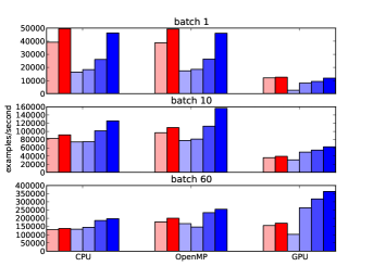
(a) Logistic regression

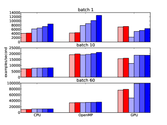
(b) Neural network, 1 hidden layer with 500 units

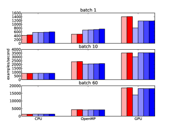
(c) Deep neural network, 3 hidden layers with 1000 units each

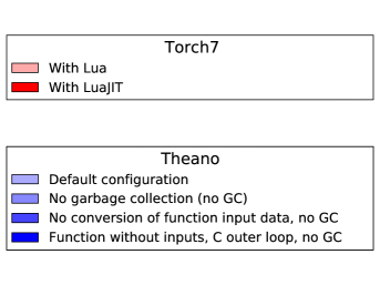
Figure 1: Benchmarks of Torch7 (red, left) vs. Theano (blue, right), for training neural networks. The bars represent examples per second, higher is better. For each architecture (a), (b), and (c), top figures represent stochastic gradient descent, middle and bottom ones use mini-batches of sizes (resp.) 10 and 60. The group of bars on the left shows performance on CPU with one thread only, the middle group shows the parallelized version with OpenMP, using 4 CPU threads, and the right-most show performance on GPU.

4.2.2 How to boost Theano’s performance

In Figure 1, the left-most blue bar (lightest shade of blue) in each of the bar groups shows the performance of a Theano function with the default configuration. That default configuration includes the use of the CVM (section 3.3), and asynchronous execution of GPU ops (section 3.7). This section shows ways to further speed up the execution, while trading off other features.

Disabling garbage collection

We can save time on memory allocation by disabling garbage collection of intermediate results. This can be done by using the linker cvm_nogc. In this case, the results of intermediate computation inside a Theano function will not be deallocated, so during the next call to the same function, this memory will be reused, and new memory will not have to be allocated. This increases memory usage, but speeds up execution of the Theano function.

In Figure 1, the second-to-left blue bar shows the impact of disabling garbage collection. It is most important on the GPU, because the garbage-collection mechanism forces a synchronization of the GPU threads, largely negating the benefits of asynchronous kernel execution.

Removing overhead of data conversion

When a Theano function is called and the data type of the provided input is different from the expected one, a silent conversion is automatically done (if no precision would be lost). For instance, a list of integers will be converted into a vector of floats, but floats will not be converted into integers (an error will be raised).

This is a useful feature, but checking and converting the input data each time the function is called can be detrimental to performance. It is now possible to disable these checks and conversions, which gives better performance when the input data is actually of the correct type. If the input data would actually need to be converted, then some exceptions due to unexpected data types will be raised during the execution. To disable these checks, simply set the trust_input attribute of a compiled Theano function to True. The third blue bar on Figure 1 shows the speed up gained with this optimization, including the cvm_nogc optimization.

Executing several iterations at once

When a Theano function does not have any explicit input (all the necessary values are stored in shared variables, for instance), we can save even more overhead by calling its fn member: f.fn(). It is also possible to call the same function multiple consecutive times, by calling f.fn(n_calls=N), saving more time. This allows to bypass the Python loop, but it will only return the results of the last iteration. This restriction means that it cannot be used everywhere, but it is still useful in some cases, for instance training a learning algorithm by iterating over a data set, where the important thing is the updates to the parameters, not the function’s output. The performance of this last way of calling a Theano function is shown in the right-most, dark blue bar.

4.2.3 Results

Figure 1 shows speed results (in example per second, higher is better) on three neural network learning tasks, which consists in 10-class classification of a 784-dimensional input. Figure 1a shows simple logistic regression, Figure 1b shows a neural network with one layer of 500 hidden units, and Figure 1c shows a deep neural network, with 3 layers of 1000 hidden units each. Torch7 was tested with the standard Lua interpreter (pale red bars), and LuaJIT, a Lua just-in-time compiler (darker red bars); Theano was tested with different optimizations (shades of blue), described in section 4.2.2.

When not using mini-batches, on CPU, Theano beats Torch7 on the models with at least one hidden layer, and even benefits from BLAS parallel implementation. On the logistic regression benchmark, Torch7 has the advantage, due to the small amount of computation being done in each call (executing several iterations at once help, but not enough to beat LuaJIT). Torch7 also has an edge over Theano on the GPU, when the batch size is one.

When using mini-batches, whether of size 10 or 60, Theano is faster than Torch7 on all three architectures, or has an equivalent speed. The difference vanishes for the most computationally-intensive tasks, as the language and framework overhead becomes negligible.

4.3 Benchmarking on Recurrent Neural Networks

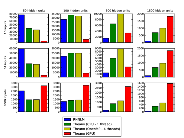
Figure 2: Benchmarks of RNNLM vs. Theano on recurrent neural networks. Reported numbers are sequence elements per second (bigger is better). The number of input units and output units is the same as the number of input units.

In Figure 2, we present a benchmark of a simple recurrent network, on Theano and RNNLM, a C++ implementation of recurrent networks for language modeling. They were done with a batch size of 1, which is customary with recurrent neural networks.

While RNNLM is faster than Theano on smaller models, Theano quickly catches up for bigger sizes, showing that Theano is an interesting option for training recurrent neural networks in a realistic scenario. This is mostly due to overhead in Theano, which is a drawback of the flexibility provided for recurrent models.

5 Conclusion

We presented recent additions to Theano, and showed how they make it a more powerful tool for machine learning software development, and allow it to be faster than competing software in most cases, on different benchmarks.

These benchmarks aim at exposing relative strengths of existing software, so that users can choose what suits their needs best. We also hope such benchmarks will help improving the available tools, which can only have a positive effect for the research community.

References

- Bergstra et al. (2010) Bergstra, J., Breuleux, O., Bastien, F., Lamblin, P., Pascanu, R., Desjardins, G., Turian, J., Warde-Farley, D., and Bengio, Y. (2010). Theano: a CPU and GPU math expression compiler. In Proceedings of the Python for Scientific Computing Conference (SciPy). Oral Presentation.
- Bergstra et al. (2011) Bergstra, J., Bastien, F., Breuleux, O., Lamblin, P., Pascanu, R., Delalleau, O., Desjardins, G., Warde-Farley, D., Goodfellow, I., Bergeron, A., and Bengio, Y. (2011). Theano: Deep learning on gpus with python. In Big Learn workshop, NIPS’11.
- Collobert et al. (2011) Collobert, R., Kavukcuoglu, K., and Farabet, C. (2011). Torch7: A matlab-like environment for machine learning. In BigLearn, NIPS Workshop.
- Hunter (2007) Hunter, J. D. (2007). Matplotlib: A 2d graphics environment. Computing in Science and Engineering, 9(3), 90–95.
- Jones et al. (2001) Jones, E., Oliphant, T., Peterson, P., et al. (2001). SciPy: Open source scientific tools for Python.
- Martens and Sutskever (2011) Martens, J. and Sutskever, I. (2011). Learning recurrent neural networks with hessian-free optimization. In L. Getoor and T. Scheffer, editors, Proceedings of the 28th International Conference on Machine Learning (ICML-11), ICML ’11, pages 1033–1040, New York, NY, USA. ACM.
- Mikolov et al. (2011) Mikolov, T., Deoras, A., Kombrink, S., Burget, L., and Cernocky, J. (2011). Empirical evaluation and combination of advanced language modeling techniques. In Proc. 12th annual conference of the international speech communication association (INTERSPEECH 2011).
- Oliphant (2007) Oliphant, T. E. (2007). Python for scientific computing. Computing in Science and Engineering, 9, 10–20.
- Pearlmutter (1994) Pearlmutter, B. A. (1994). Fast exact multiplication by the hessian. Neural Computation, 6, 147–160.
- Pérez and Granger (2007) Pérez, F. and Granger, B. E. (2007). IPython: A system for interactive scientific computing. Computing in Science and Engineering, 9(3), 21–29.
- Rumelhart et al. (1986) Rumelhart, D. E., Hinton, G. E., and Williams, R. J. (1986). Learning internal representations by error propagation. volume 1, chapter 8, pages 318–362. MIT Press, Cambridge.