Abstract

We study the inverse problem for the so-called operators with energy depending potentials. In particular, we study spectral operators with quadratic dependance on the spectral parameter. The corresponding hierarchy of integrable equations includes the Kaup-Bousinesq equation. We formulate the inverse problem as a Riemann-Hilbert problem with a $\mathbb{Z}_{2}$ reduction group. The soliton solutions are explicitly obtained.

PACS: 05.45.Yv, 02.20.Sv

Key Words: Inverse Scattering Method, Nonlinear Evolution Equations, Solitons.

1 Introduction

The last decades witnessed an explosion in the complexity and sophistication of mathematical theories for fluids and in particular for water waves. The soliton theory has been always at the center of these developments, such as from its early days the soliton theory has transformed and enhanced enormously the mathematical description of nonlinear wave propagation. The simplest and best known integrable water-wave equations belong to the Korteweg-de Vries family. For some classical and modern aspects of the theory of water waves, nonlinear waves and soliton theory we refer to the following monographs and the references therein: [1, 5, 9, 10, 13, 20, 26, 28, 30, 31].

There are classes of soliton equations whose associated spectral problems are polynomial in the spectral parameter. They are known also as soliton equations with ’energy dependent potentials’ due to the analogy with the Schrödinger equation in Quantum Mechanical context, whose spectrum represents the energy levels of the Quantum Mechanical system. Some of these integrable systems appear as water waves models, most notably the Kaup-Boussinesq equation [22, 30, 7] and the two-component Camassa-Holm equation [6, 13, 12, 15]. Other systems of this type are studied e.g. in [2, 3, 14, 4].

In what follows we study an integrable system which arises as a compatibility condition of the following two linear operators (Lax pair):

$$\Psi_{xx}=\left(-\lambda^{2}+\lambda u(x,t)+\frac{\kappa}{2}u^{2}(x,t)+\eta(x,t)\right)\Psi(x,t;\lambda)$$ (1)

$$\Psi_{t}=-\left(\lambda+\frac{1}{2}u(x,t)\right)\psi_{x}(x,t;\lambda)+\frac{1}{4}u_{x}(x,t)\Psi(x,t;\lambda).$$ (2)

Here $\kappa$ is an arbitrary constant, while $\lambda$ is the spectral parameter. The consistency condition $\psi_{xxt}(x,t;\lambda)=\psi_{txx}(x,t;\lambda)$ produces a system of equations for the functions $u(x,t)$ and $\eta(x,t)$:

$$u_{t}+\eta_{x}+\left(\frac{3}{2}+\kappa\right)uu_{x}=0,$$ (3)

$$\eta_{t}-\frac{1}{4}u_{xxx}+(u\eta)_{x}-\left(\frac{1}{2}+\kappa\right)u\eta_{x}-\kappa\left(\frac{1}{2}+\kappa\right)u^{2}u_{x}=0.$$ (4)

Upon choosing $\kappa=-\frac{1}{2}$ these simplify to the well known Kaup-Boussinesq (or KB for short) equation:

$$u_{t}+\eta_{x}+uu_{x}=0,$$ (5)

$$\eta_{t}-\frac{1}{4}u_{xxx}+(u\eta)_{x}=0.$$ (6)

The KB equation is introduced as a water-wave model in [22] where also the inverse scattering is studied for functions with constant limits at $x\to\pm\infty$. As a water-wave model it also appears in [30, 15, 7, 11], the hierarchy of Hamiltonian structurs is given in [27], specific solutions are studied in [21, 8, 24]. Energy-dependant spectral problems like (1) are studied also in [16, 17, 18, 19, 24, 29, 23].

Our aim will be to formulate the inverse scattering as a Riemann-Hilbert Problem (RHP) in the case when $u(x,t)$ and $\eta(x,t)$ are real, rapidly decaying functions at $x\to\pm\infty$, taking into account the underlying reductions and to obtain the simplest soliton solutions.

2 The spectral problem

Introducing an auxiliary function

$$w(x,t)=\frac{\kappa}{2}u^{2}(x,t)+\eta(x,t)$$ (7)

we consider the following two ’conjugate’ spectral problems related to (1):

$$\Psi_{xx}(x,\lambda,\sigma)=\left(-\lambda^{2}+\sigma\lambda u(x)+w(x)\right)\Psi(x,\lambda,\sigma),$$ (8)

where $\sigma=\pm 1$. The $t$-dependence will be suppressed where possible for the sake of simplicity.

We specify that $u(x),w(x)$ as well as $\eta(x)$ belong the the Schwartz class of functions (the space of rapidly decreasing functions) $\mathcal{S}(\mathbb{R})$. It follows from this requirement, that solutions $\psi_{1}(x,t;\lambda)$ and $\psi_{2}(x,t;\lambda)$ exist such that,

$$\begin{array}[]{c}\psi_{1}(x,\lambda,\sigma)\to e^{-i\lambda x}\\ \psi_{2}(x,\lambda,\sigma)\to e^{+i\lambda x}\\ \end{array}\Bigg{\}},\quad x\to+\infty$$ (9)

Similarly we define a basis of eigenfunctions for (8) according to

$$\begin{array}[]{c}\phi_{1}(x,\lambda,\sigma)\to e^{-i\lambda x}\\ \phi_{2}(x,\lambda,\sigma)\to e^{+i\lambda x}\\ \end{array}\Bigg{\}},\quad x\to-\infty$$ (10)

These eigenfunctions are called Jost Solutions. Since the Jost solutions oscillate when $\lambda\in\mathbb{R}$, the real spectrum fills in the real line.

The bases $\{\psi_{1}(x,\lambda,\sigma),\psi_{2}(x,\lambda,\sigma)\}$ and $\{\phi_{1}(x,\lambda,\sigma),\phi_{2}(x,\lambda,\sigma)\}$ constitute independent bases of solutions to (8) and as such, we may write

$$\left(\begin{array}[]{c}\phi_{1}(x,\lambda,\sigma)\\ \phi_{2}(x,\lambda,\sigma)\\ \end{array}\right)=\left(\begin{array}[]{cc}T_{11}(\lambda,\sigma)&T_{12}(\lambda,\sigma)\\ T_{21}(\lambda,\sigma)&T_{22}(\lambda,\sigma)\\ \end{array}\right)\left(\begin{array}[]{c}\psi_{1}(x,\lambda,\sigma)\\ \psi_{2}(x,\lambda,\sigma)\\ \end{array}\right).$$ (17)

The matrix

$$\mathbf{T}(\lambda,\sigma)=\left(\begin{array}[]{cc}T_{11}(\lambda,\sigma)&T_{12}(\lambda,\sigma)\\ T_{21}(\lambda,\sigma)&T_{22}(\lambda,\sigma)\\ \end{array}\right)$$ (18)

is the scattering matrix for spectral problem (8).

Under the involution $(\lambda,\sigma)\to(-\lambda,-\sigma),$ the potential in (8) remains invariant. Therefore the eigenfunctions $\psi(x,\lambda,\sigma)$ and $\psi(x,-\lambda,-\sigma)$ are solutions to the same spectral problem. Since the asymptotics of these solutions do not depend on $\sigma$, it follows that

$$\psi_{1}(x,\lambda,\sigma) = \psi_{2}(x,-\lambda,-\sigma)$$

$$\phi_{1}(x,\lambda,\sigma) = \phi_{2}(x,-\lambda,-\sigma),$$ (19)

Thus, we can write the two bases using just one of the functions, say $\psi(x,\lambda,\sigma)\equiv\psi_{1}(x,\lambda,\sigma)$ and $\phi(x,\lambda,\sigma)\equiv\phi_{1}(x,\lambda,\sigma)$ as $\psi_{2}(x,\lambda,\sigma)=\psi(x,-\lambda,-\sigma)$ and $\phi_{2}(x,\lambda,\sigma)\equiv\phi(x,-\lambda,-\sigma)$.

When $u(x,t)$ and $\eta(x,t)$ are real, the spectral problem (8) is invariant under $\mathbb{Z}_{2}$ reduction group [25], i.e. it has the following property: if $\psi(x,\lambda,\sigma)$ is an eigenfunction, so is $\bar{\psi}(x,\bar{\lambda},\sigma)$. Comparing the asymptotics again, we conclude that this coinsides with the second Jost solution, i.e.

$$\bar{\psi}(x,\bar{\lambda},\sigma)=\psi(x,-\lambda,-\sigma)$$ (20)

Thus, for $\lambda\in\mathbb{R}$ we also have $\psi(x,\lambda,\sigma)=\bar{\psi}(x,-\lambda,-\sigma)$. From this, and (17) it follows that the scattering matrix $\mathbf{T}(\lambda)$ may be written in the form

$$\mathbf{T}(\lambda,\sigma)=\left(\begin{array}[]{cc}a(\lambda,\sigma)&b(\lambda,\sigma)\\ \bar{b}(\lambda,\sigma)&\bar{a}(\lambda,\sigma)\end{array}\right),$$ (21)

for spectral parameter $\lambda\in\mathbb{R}.$

We now have the following relationship between $\phi(x,\lambda,\sigma)$ and the Jost solutions $\psi(x,\lambda,\sigma),\bar{\psi}(x,\lambda,\sigma),$

$$\phi(x,\lambda,\sigma)=a(\lambda,\sigma)\psi(x,\lambda,\sigma)+b(\lambda,\sigma)\psi(x,-\lambda,-\sigma).$$ (22)

Furthermore, for any pair of solutions $f_{1}$ and $f_{2}$ to (8) the Wronskian of the pair is independent of $x$,

$$\partial_{x}W[f_{1},f_{2}]=\partial_{x}(f_{1}\partial_{x}f_{2}-f_{2}\partial_{x}f_{1})=0.$$

In particular, it follows that the Jost solutions satisfy the following condition

$$W[\phi(x,\lambda,\sigma),\bar{\phi}(x,\lambda,\sigma)]=W[\psi(x,\lambda,\sigma),\bar{\psi}(x,\lambda,\sigma)]=2i\lambda,$$ (23)

which clearly follows from the asymptotic behaviour of $\{\psi(x,\lambda,\sigma)\bar{\psi}(x,\lambda,\sigma)\}$ and $\{\phi(x,\lambda,\sigma),\bar{\phi}(x,\lambda,\sigma)\}$ as $|x|\to\infty.$ It follows from (22) and (23) that

$$\det\mathbf{T(\lambda,\sigma)}=|a(\lambda,\sigma)|^{2}-|b(\lambda,\sigma)|^{2}=1,\qquad\lambda\in\mathbb{R}.$$ (24)

3 Asymptotic behaviour of the Jost solutions

Since the functions $u(x)$ and $w(x)$ are Schwartz class it follows that the solution $\psi(x,\lambda,\sigma)$ have asymptotic behaviour such that

$$\psi_{xx}(x,\lambda,\sigma)\to-\lambda^{2}e^{-i\lambda x},\quad x\to+\infty.$$ (25)

Consequently, we make the following ansatz for the asymptotic expansion as $|\lambda|\to\infty$,

$$\psi(x,\lambda,\sigma)=\left[X_{0}(x,\sigma)+\frac{1}{\lambda}X_{1}(x,\sigma)+\mathcal{O}(\lambda^{-2})\right]e^{-i\lambda x},$$ (26)

where the function $X_{0}(x,\sigma)$ and $X_{1}(x,\sigma)$ behave asymptotically according to

$$\begin{array}[]{c}X_{0}(x,\sigma)\to 1\\ X_{1}(x,\sigma)\to 0\end{array}\Bigg{\}},\quad x\to+\infty.$$ (27)

The substitution of (26) into (8) gives

$$\frac{\partial_{x}X_{0}(x,\sigma)}{X_{0}(x,\sigma)} = \frac{i}{2}\sigma u(x),$$ (28)

$$\sigma u(x)X_{1}(x,\sigma)+2i\partial_{x}X_{1}(x,\sigma) = -w(x)\cdot X_{0}(x,\sigma)+\partial_{x}^{2}X_{0}(x,\sigma).$$ (29)

Using the conditions in (27) we may easily solve (28), (29) to give the following expressions for $X_{0}(x,\sigma)$ and $X_{1}(x,\sigma)$:

$$X_{0}(x,\sigma) = \exp\left\{-\frac{i\sigma}{2}\int_{x}^{\infty}u(x^{\prime})dx^{\prime}\right\},$$

$$X_{1}(x,\sigma) = X_{0}(x,\sigma)\cdot\left[\frac{\sigma}{4}u(x)-\frac{i}{8}\int_{x}^{\infty}(u^{2}(x^{\prime})+4w(\xi))dx^{\prime}\right].$$ (30)

Similarly, we obtain analogous expressions for $\psi(x,\lambda,\sigma)$, i.e.

$$\psi(x,\lambda,\sigma) = e^{-i\left(\lambda x+\frac{\sigma}{2}\int_{x}^{\infty}u(x^{\prime})dx^{\prime}\right)}\left[1+\frac{1}{\lambda}\xi_{1}(x,\sigma))+\ldots\right],$$ (31)

$$\phi(x,\lambda,\sigma) = e^{-i\left(\lambda x-\frac{\sigma}{2}\int^{x}_{-\infty}u(x^{\prime})dx^{\prime}\right)}\left[1+\frac{1}{\lambda}\zeta_{1}(x,\sigma)+\ldots\right],$$ (32)

where the functions $\xi_{1}(x)$ and $\zeta_{1}(x)$ are given by

$$\xi_{1}(x,\sigma) = \frac{\sigma}{4}u(x)-\frac{i}{8}\int^{\infty}_{x}(u^{2}(x^{\prime})+4w(x^{\prime}))dx^{\prime},$$

$$\zeta_{1}(x,\sigma) = \frac{\sigma}{4}u(x)+\frac{i}{8}\int_{-\infty}^{x}(u^{2}(x^{\prime})+4w(x^{\prime}))dx^{\prime}.$$ (33)

4 Analytic behaviour of the Jost solutions

We now define the related function

$$\chi^{(+)}(x,\lambda,\sigma)=e^{i\lambda x}\phi(x,\lambda,\sigma)\to 1,\quad x\to-\infty.$$ (34)

Using

$$e^{i\lambda x}\phi_{x}(x,\lambda,\sigma)=\chi_{x}^{(+)}(x,\lambda,\sigma)-i\lambda\chi^{(+)}(x,\lambda,\sigma)$$

along with the spectral problem in (8), we may write

$$\chi_{xx}^{(+)}(x,\lambda,\sigma)=(\lambda\sigma u(x)+w(x))\chi^{(+)}(x,\lambda,\sigma)+2i\lambda\chi_{x}^{(+)}(x,\lambda,\sigma).$$ (35)

Meanwhile the asymptotic expansion in $\lambda$ appearing in (32) suggests the following integral representation for $\chi^{(+)}(x,\lambda,\sigma),$

$$\chi^{(+)}(x,\lambda,\sigma)=1+\int_{-\infty}^{x}\frac{e^{2i\lambda(x-x^{\prime})}-1}{2i\lambda}P(x^{\prime},\lambda,\sigma)\chi^{(+)}(x^{\prime},\lambda,\sigma)dx^{\prime}$$ (36)

for some $P(x,\lambda,\sigma)\in\mathcal{S}(\mathbb{R})$. From this integral representation differentiating twice we obtain

$$\chi^{(+)}_{xx}(x,\lambda,\sigma) = P(x,\lambda,\sigma)\chi^{(+)}(x,\lambda,\sigma)+2i\lambda\chi^{(+)}_{x}(x,\lambda,\sigma).$$

From (35) and (4) we determine

$$P(x,\lambda,\sigma)=\lambda\sigma u(x)+w(x),$$ (37)

and so we may write

$$\chi^{(+)}(x,\lambda,\sigma)=1+\int_{-\infty}^{x}\frac{e^{2i\lambda(x-x^{\prime})}-1}{2i\lambda}(\lambda\sigma u(x^{\prime})+w(x^{\prime}))\chi^{(+)}(x^{\prime},\lambda,\sigma)dx^{\prime}.$$ (38)

Of particular importance and clear from (38) is the analytic properties of $\chi^{(+)}(x,\lambda,\sigma)$. We can see that for all values of $x$ the kernel of the integral above is finite for all values of $\lambda$ such that $\mbox{Im }\lambda>0.$ Therefore $\chi^{(+)}(x,\lambda,\sigma)$ and $\phi(x,\lambda,\sigma)$ are analytic in the upper half plane $\mathbb{C}_{+}$. It obviously follows that $\bar{\chi}^{(+)}(x,\bar{\lambda},\sigma)$ is analytic for $\lambda\in\mathbb{C}_{-}$.

In a similar manner we may define

$$\chi^{(-)}(x,\lambda,\sigma)=e^{i\lambda x}\psi(x,\lambda,\sigma)\to 1,\quad x\to+\infty$$ (39)

from which it follows that

$$\chi^{(-)}(x,\lambda,\sigma)=1-\int_{x}^{\infty}\frac{e^{2i\lambda(x-x^{\prime})}-1}{2i\lambda}(\lambda\sigma u(x)+w(x))\chi^{(-)}(x,\lambda,\sigma).$$ (40)

It is immediately clear from (40) that $\chi^{(-)}(x,\lambda,\sigma)$ and therefore $\psi(x,\lambda,\sigma)$ are analytic throughout $\mathbb{C}_{-}.$

Next we introduce new notation for later convenience,

$$\omega_{-}(x)=\frac{1}{2}\int_{-\infty}^{x}u(x^{\prime})dx^{\prime}\quad\mbox{and}\quad\omega_{+}(x)=\frac{1}{2}\int_{x}^{\infty}u(x^{\prime})dx^{\prime}.$$ (41)

With this we may rewrite (31), (32) as follows

$$\underline{\psi}(x,\lambda,\sigma)=\psi(x,\lambda,\sigma)e^{i(\lambda x+\sigma\omega_{+}(x))}=1+\frac{1}{\lambda}\xi_{1}(x,\sigma),$$

$$\underline{\phi}(x,\lambda,\sigma)=\phi(x,\lambda,\sigma)e^{i(\lambda x-\sigma\omega_{-}(x))}=1+\frac{1}{\lambda}\zeta_{1}(x,\sigma).$$ (42)

To obtain the analytic properties of $\underline{\psi}(x,\lambda,\sigma)$ and $\underline{\phi}(x,\lambda,\sigma),$ we note that

$$\underline{\psi}(x,\lambda,\sigma)=\chi^{(-)}(x,\lambda,\sigma)e^{i\sigma\omega_{+}(x)}\quad\mbox{and}\quad\underline{\phi}(x,\lambda,\sigma)=\chi^{(+)}(x,\lambda,\sigma)e^{-i\sigma\omega_{-}(x)}.$$

Since $u(x)$ is Schwartz class and independent of $\lambda$ and given the analyticity of $\chi^{(\pm)}(x,\lambda,\sigma)$ throughout $\mathbb{C}_{\pm}$ respectively, it follows that $\underline{\phi}(x,\lambda,\sigma)$ and $\underline{\psi}(x,\lambda,\sigma)$ are also analytic throughout $\mathbb{C}_{+}$ and $\mathbb{C}_{-}$ respectively.

5 The $t$-dependence of the scattering data

We may rewrite the second member of the Lax pair in terms of the auxiliary function $u(x)$ and add an arbitrary constant $\gamma,$ without effecting the physical equations of motion, to obtain,

$$\Psi_{t}(x,\lambda,\sigma)=-\left(\sigma\lambda+\frac{1}{2}u(x)\right)\Psi_{x}(x,\lambda,\sigma)+\left(\gamma+\frac{1}{4}u_{x}(x)\right)\Psi(x,\lambda,\sigma).$$ (43)

In particular we may write

$$\phi_{t}(x,\lambda,\sigma)=-\left(\sigma\lambda+\frac{1}{2}u(x)\right)\phi_{x}(x,\lambda,\sigma)+\left(\gamma+\frac{1}{4}u_{x}(x)\right)\phi(x,\lambda,\sigma).$$ (44)

However, we also note that along the discrete spectrum we have the scattering relation (22), from which we may obtain the asymptotic behavior of $\phi_{t}(x,\lambda,\sigma)$ as $x\to+\infty,$ namely

$$\phi_{t}(x,\lambda,\sigma)\to a_{t}(\lambda,\sigma)e^{-i\lambda x}+b_{t}(\lambda,\sigma)e^{+i\lambda x}.$$ (45)

Using the r.h.s of (44) along with (22), we find as $x\to+\infty$ that

$$\phi_{t}(x,\lambda,\sigma)\to - \sigma\lambda[-i\lambda a(\lambda,\sigma)e^{-i\lambda x}+i\lambda b(\lambda,\sigma)e^{i\lambda x}]$$ (46)

$$+ \gamma[a(\lambda,\sigma)e^{-i\lambda x}+b(\lambda,\sigma)e^{+i\lambda x}],$$

where we have made use of the fact that $u(x)$ is Schwartz class and vanishes when $x\to\pm\infty$. Making the choice $\gamma=-i\sigma\lambda^{2},$ the $t$-derivative of $a(\lambda,\sigma)$ vanishes. It follows that we may write

$$\begin{array}[]{c}a_{t}(\lambda,\sigma)=0\Rightarrow a(\lambda,\sigma,t)=a(\lambda,\sigma,0),\\ b_{t}(\lambda,\sigma)=-2i\lambda^{2}b(\lambda,\sigma)\Rightarrow b(\lambda,\sigma,t)=b(\lambda,\sigma,0)e^{-2i\sigma\lambda^{2}t}.\end{array}$$ (47)

Along the discrete spectrum, we have $a(\lambda_{n},\sigma)=0$ and therefore instead of (45) we have

$$\phi_{t}(x,\lambda_{n},\sigma)\to b_{n,t}(\sigma)e^{i\lambda_{n}x}.$$ (48)

Instead of (46) we have

$$\phi_{t}(x,\lambda_{n},\sigma)\to-\sigma\lambda_{n}[i\lambda_{n}b_{n}(\sigma)e^{i\lambda_{n}x}]+\gamma(\lambda_{n})b_{n}(\sigma)e^{i\lambda_{n}x},$$ (49)

and thus

$$b_{n,t}(\sigma)=-2i\sigma\lambda_{n}^{2}b_{n}(\sigma),$$ (50)

from where

$$b_{n}(\sigma,t)=b_{n}(\sigma,0)e^{-2i\sigma\lambda_{n}^{2}t}.$$ (51)

6 Conservation Laws

We may derive a collection of conserved quantities from the spectral problem introduced in the previous section in (8). To proceed we first introduce the function

$$\rho(x,\lambda,\sigma)=\frac{\Psi_{x}(x,\lambda,\sigma)}{\Psi(x,\lambda,\sigma)}.$$ (52)

Differentiating once with respect to $x$ we find

$$\rho^{2}+\rho_{x}=-\lambda^{2}+\sigma\lambda u+w.$$ (53)

Using this result, along with the Lax pair in (8) and (43) we find upon differentiating (52) with respect to $t$ that

$${}\rho_{t}=\frac{1}{4}\left(u_{x}-2\rho u-4\sigma\lambda\rho\right)_{x}.$$ (54)

Using the the fact $u(x)$ and $w(x)$ are Schwartz class, we see from (54) that

$${\int_{-\infty}^{+\infty}}\rho_{t}(x,\lambda,\sigma)dx=0,$$ (55)

that is to say

$$\mathcal{I}_{0}(\lambda)=\displaystyle{\int_{-\infty}^{+\infty}}\rho(x,\lambda,\sigma)dx$$ (56)

is a generating function for the conserved quantities. We may expand it in a power series in $\lambda$ according to

$$\mathcal{I}_{0}=\lambda\mathcal{I}_{1}+\mathcal{I}_{2}+\frac{\mathcal{I}_{3}}{\lambda}+\frac{\mathcal{I}_{4}}{\lambda^{2}}+\mathcal{O}(\lambda^{-3}),$$ (57)

where $\mathcal{I}_{1},\mathcal{I}_{2},$ etc is an infinite sequence of conserved quantities. Next, we expand $\rho(x,t,\lambda)$ as a power series in $\lambda$

$$\rho(x,\lambda,\sigma)=i\lambda+\rho_{0}(x)+\frac{\rho_{1}(x,t)}{\lambda}+\frac{\rho_{2}(x)}{\lambda^{2}}+\mathcal{O}(\lambda^{-3}),$$ (58)

and use it in (53), then the terms of equivalent order in $\lambda$ give

$$\rho_{0}(x)=-\frac{i\sigma}{2}u(x)$$ (59)

and as a result of (57) it follows that

$$\mathcal{I}_{2}=\int_{-\infty}^{+\infty}\rho_{0}(x)dx=-\frac{i\sigma}{2}\int_{-\infty}^{+\infty}u(x)dx.$$ (60)

So we see that

$$\alpha_{1}\equiv\frac{1}{2}\int_{-\infty}^{+\infty}u(x)dx$$ (61)

is an integral of motion. Following a similar procedure, we find the next conserved quantities to be

$$\mathcal{I}_{3}=-\frac{i}{8}\int_{-\infty}^{+\infty}(u^{2}(x)+4w(x))dx,$$

$$\mathcal{I}_{4}=-\frac{i\sigma}{16}\int_{-\infty}^{+\infty}u(x)(u^{2}(x)+4w(x))dx.$$ (62)

One may continue a process of iteration indefinitely, whereby an infinite series of such conserved quantities is generated from the $u(x)$ and $w(x),$ and therefore from the physical variables $u(x)$ and $\eta(x)$.

7 Analytic continuation of $a(\lambda,\sigma)$

Returning to (22) we see that we may re-write the scattering coefficient $a(\lambda,\sigma)$ in terms of the $x$-independent Wronsikian,

$$a(\lambda,\sigma)=\frac{W[\phi(x,\lambda,\sigma),\psi(x,-\lambda,-\sigma)]}{2i\lambda}.$$ (63)

Since the two eigenfunctions in (63) are analytic for $\lambda\in\mathbb{C}_{+}$, $a(\lambda,\sigma)$ allows an analytic continuation in the upper half complex plane. From (63) with (31)– (32) we obtain the asymptotic behavior of the scattering coefficient,

$$\lim_{|\lambda|\to\infty}a(\lambda,\sigma)=e^{i\sigma\alpha_{1}}$$ (64)

where $\alpha_{1}$ is the conserved quantity (61). We make further the assumption that $a(\lambda,\sigma)$ has a finite number of simple zeros $\lambda_{n}\in\mathbb{C}_{+}$, $n=1,2,3,\ldots,N$. We introduce the auxiliary function

$$A(\lambda,\sigma)=e^{-i\sigma\alpha_{1}}\displaystyle{\prod_{n=1}^{N}}\frac{\lambda-\bar{\lambda}_{n}}{\lambda-\lambda_{n}}a(\lambda,\sigma),$$ (65)

which is analytic without zeroes in $\mathbb{C}_{+}$. It follows from (65) that

$$|A(\lambda,\sigma)|=|a(\lambda,\sigma)|,\quad\lambda\in\mathbb{R},$$ (66)

Next, we also see from (64) and (65) that

$${\lim_{|\lambda|\to\infty}}\ln A(\lambda,\sigma)=0,$$ (67)

and so, $\ln A(\lambda,\sigma)$ is analytic throughout $\mathbb{C}_{+}$ and vanishes as $|\lambda|\to\infty.$

We also have from (66)

$$\ln A(\lambda,\sigma)=\ln|A(\lambda,\sigma)|+i\arg A(\lambda,\sigma)=\ln|a(\lambda,\sigma)|+i\arg A(\lambda,\sigma),$$

for $\lambda\in\mathbb{R}.$ We make use of the Kramers-Kronig dispersion relations,

$$\ln|a(\lambda,\sigma)|=\frac{1}{\pi}\fint\limits_{-\infty}^{\infty}\frac{\arg A(\lambda^{\prime},\sigma)}{\lambda^{\prime}-\lambda}d\lambda^{\prime}$$

$$\arg{A(\lambda,\sigma)}=-\frac{1}{\pi}\fint\limits_{-\infty}^{\infty}\frac{\ln|a(\lambda^{\prime},\sigma)|}{\lambda^{\prime}-\lambda}d\lambda^{\prime},$$ (68)

for $\lambda\in\mathbb{R},$ where the dashed integral denoted the principal value part of the integral. Then with (7) we have

$$\ln A(\lambda,\sigma) = \ln|a(\lambda,\sigma)|-\frac{i}{\pi}\fint\limits_{-\infty}^{\infty}\frac{\ln|a(\lambda^{\prime},\sigma)|}{\lambda^{\prime}-\lambda}d\lambda^{\prime}$$ (69)

$$= \frac{1}{\pi i}\int\limits_{-\infty}^{\infty}\frac{\ln|a(\lambda^{\prime},\sigma)|}{\lambda^{\prime}-\lambda-i0^{+}}d\lambda^{\prime},\qquad\lambda\in\mathbb{R}.$$

Meanwhile, (65) gives

$$\ln A(\lambda,\sigma)=-i\sigma\alpha_{1}-\displaystyle\sum_{n=1}^{N}\frac{\lambda-\lambda_{n}}{\lambda-\bar{\lambda}_{n}}+\ln a(\lambda,\sigma).$$ (70)

Using (69) and (70), we find that for real values of $\lambda$ we may write

$$\ln a(\lambda,\sigma)=i\sigma\alpha_{1}+\displaystyle\sum_{n=1}^{N}\frac{\lambda-\lambda_{n}}{\lambda-\bar{\lambda}_{n}}+\frac{1}{\pi i}\int\limits_{-\infty}^{\infty}\frac{\ln|a(\lambda^{\prime},\sigma)|}{\lambda^{\prime}-\lambda-i0^{+}}d\lambda^{\prime}$$ (71)

and for $\lambda\in\mathbb{C}_{+}$ the analytical continuation is

$$\ln a(\lambda,\sigma)=i\sigma\alpha_{1}+\displaystyle\sum_{n=1}^{N}\frac{\lambda-\lambda_{n}}{\lambda-\bar{\lambda}_{n}}+\frac{1}{\pi i}\int\limits_{-\infty}^{\infty}\frac{\ln|a(\lambda^{\prime},\sigma)|}{\lambda^{\prime}-\lambda}d\lambda^{\prime}.$$ (72)

8 The Riemann-Hilbert problem

We may re-write the expression (22) in terms of the new analytic functions $\underline{\phi}(x,\lambda,\sigma),\underline{\psi}(x,\lambda,\sigma)$ using (20) for $\lambda\in\mathbb{R},$ as follows

$$\frac{\underline{\phi}(x,\lambda,\sigma)e^{i\sigma\alpha_{1}}}{a(\lambda,\sigma)}=\underline{\psi}(x,\lambda\,\sigma)+r(\lambda,\sigma)\underline{\bar{\psi}}(x,\lambda,\sigma)e^{2i(\lambda x+\sigma\omega_{+}(x))},$$ (73)

$r(\lambda,\sigma)=b(\lambda,\sigma)/a(\lambda,\sigma)$. The function $\frac{\underline{\phi}(x,\lambda,\sigma)e^{i\sigma\alpha_{1}}}{a(\lambda,\sigma)}$ is analytic for $\mathrm{Im}\phantom{*}\lambda>0$, while $\underline{\psi}(x,\lambda\,\sigma)$ is analytic for $\mathrm{Im}\phantom{*}\lambda<0$. Thus, equation (73) represents an additive Riemann-Hilbert Problem (RHP) with a jump on the real line, given by

$$r(\lambda,\sigma)\underline{\bar{\psi}}(x,\lambda,\sigma)e^{2i(\lambda x+\sigma\omega_{+}(x))}$$

and a normalization condition $\lim_{|\lambda|\to\infty}\underline{\psi}(x,\lambda,\sigma)=X_{0}(x,\sigma)$.

In this section we will follow the standard technique for solving RHP. We integrate the two analytic functions with respect to $\oint\frac{d\lambda^{\prime}}{\lambda^{\prime}-\lambda}(\cdot)$ over the boundary of their analyticity domains, using the normalization condition. In our case the domains (the upper $\mathbb{C}_{+}$ and the lower $\mathbb{C}_{-}$ complex half-planes) have the real line as a common boundary and there we relate the integrals using the jump condition. The RHP approach for various equation is presented in [10, 23, 12, 29].

We now choose some $\lambda\in\mathbb{C}_{-}$ and integrate the left-hand side as follows,

$$\frac{1}{2\pi i}\ointctrclockwise_{C^{+}}\frac{\underline{\phi}(x,\lambda^{\prime},\sigma)e^{i\sigma\alpha_{1}}}{a(\lambda^{\prime},\sigma)\cdot(\lambda^{\prime}-\lambda)}d\lambda^{\prime}=\sum_{n=1}^{N}\frac{\underline{\phi}^{(n)}(x,\sigma)e^{i\sigma\alpha_{1}}}{\dot{a}_{n}(\sigma)\cdot(\lambda_{n}-\lambda)}$$ (74)

where $C^{+}$ is the contour in the upper half plane shown in Fig. 1,

$$\dot{a}_{n}(\sigma)\equiv\left(\frac{\text{d}a(\lambda,\sigma)}{\text{d}\lambda}\right)_{\lambda=\lambda_{n}}\neq 0,\qquad\underline{\phi}^{(n)}(x,\sigma)\equiv\underline{\phi}(x,\lambda_{n},\sigma).$$

Figure 1: The integration contours $C^{+}$ and $C^{-}$ are the closed paths in the upper and lower half planes correspondingly; $\Gamma_{\pm}$ are the semicircles with an infinite radius.

We may write the integral as such because $\lambda\in\mathbb{C}_{-}$ and so $\frac{1}{\lambda-\lambda^{\prime}}$ is analytic throughout $\mathbb{C}_{+}$. Furthermore, $a(\lambda)$ is analytic with finite number of simple zeros, $\lambda_{n}$ in $\mathbb{C}_{+},$ and the function $\underline{\phi}(x,\lambda)$ is analytic throughout $\mathbb{C}_{+}.$ Alternatively we may expand the integral as follows

$$\frac{1}{2\pi i}\ointctrclockwise_{C^{+}}\frac{\underline{\phi}(x,\lambda^{\prime},\sigma)e^{i\alpha_{1}}}{a(\lambda^{\prime},\sigma)\cdot(\lambda^{\prime}-\lambda)}d\lambda^{\prime} =$$

$$\frac{1}{2\pi i}\int_{-\infty}^{\infty}\frac{\underline{\phi}(x,\lambda^{\prime},\sigma)e^{i\alpha_{1}}}{a(\lambda^{\prime})\cdot(\lambda^{\prime}-\lambda)}d\lambda^{\prime} + \frac{1}{2\pi i}\int_{\Gamma_{+}}\frac{\underline{\phi}(x,\lambda^{\prime},\sigma)e^{i\alpha_{1}}}{a(\lambda^{\prime},\sigma)\cdot(\lambda^{\prime}-\lambda)}d\lambda^{\prime}.$$ (75)

Using the asymptotic properties of $a(\lambda,\sigma)$ and $\underline{\phi}(x,\lambda,\sigma)$ along with the relationship (73), we find

$$\sum_{n=1}^{N}\frac{\underline{\phi}^{(n)}(x,\sigma)e^{i\alpha_{1}}}{\dot{a}(\lambda_{n})\cdot(\lambda_{n}-\lambda)} = \frac{1}{2\pi i}\int_{\Gamma^{+}}\frac{1}{\lambda^{\prime}-\lambda}d\lambda^{\prime}+\frac{1}{2\pi i}\int_{-\infty}^{\infty}\frac{\underline{\psi}(x,\lambda^{\prime},\sigma)}{\lambda^{\prime}-\lambda}d\lambda^{\prime}$$

$$+ \frac{1}{2\pi i}\int_{-\infty}^{\infty}\frac{r(\lambda^{\prime},\sigma)e^{2i(\lambda^{\prime}x+\sigma\omega_{+}(x))}\underline{\bar{\psi}}(x,\lambda^{\prime},\sigma)}{\lambda^{\prime}-\lambda}d\lambda^{\prime}.$$

Next we obtain an expression for the line-integral

$$\frac{1}{2\pi i}\int_{-\infty}^{+\infty}\frac{\underline{\psi}(x,\lambda^{\prime},\sigma)}{\lambda^{\prime}-\lambda}d\lambda^{\prime},$$

by considering the integral over the contour $C^{-},$ shown in Fig. 1. Since $\lambda\in\mathbb{C}_{-}$ and $\underline{\psi}(x,\lambda,\sigma)$ is analytic therein. In addition the contour $C^{-}$ is clockwise, so it follows that

$$\frac{1}{2\pi i}\ointclockwise_{C^{-}}\frac{\underline{\psi}(x,\lambda,\sigma)}{\lambda^{\prime}-\lambda}d\lambda^{\prime}=-\psi(x,\lambda,\sigma).$$ (77)

Expanding the integral, we have

$$\frac{1}{2\pi i}\ointclockwise_{C^{-}}\frac{\underline{\psi}(x,\lambda^{\prime},\sigma)}{\lambda^{\prime}-\lambda}d\lambda^{\prime}=\frac{1}{2\pi i}\int_{-\infty}^{+\infty}\frac{\underline{\psi}(x,\lambda^{\prime},\sigma)}{\lambda^{\prime}-\lambda}d\lambda^{\prime}+\frac{1}{2\pi i}\int_{\Gamma_{-}}\frac{\underline{\psi}(x,\lambda^{\prime},\sigma)}{\lambda^{\prime}-\lambda}d\lambda^{\prime}.$$ (78)

Using the asymptotic properties of $\underline{\psi}(x,\lambda,\sigma)$ as $|\lambda|\to\infty$ with $\lambda\in\mathbb{C}^{-},$ we have,

$$\frac{1}{2\pi i}\int_{-\infty}^{\infty}\frac{\underline{\psi}(x,\lambda^{\prime},\sigma)}{\lambda^{\prime}-\lambda}d\lambda^{\prime}=-\underline{\psi}(x,\lambda,\sigma)-\frac{1}{2\pi i}\int_{\Gamma_{-}}\frac{1}{\lambda^{\prime}-\lambda}d\lambda^{\prime}$$ (79)

We can also make use of the following result when it comes to substituting this expression in (8),

$$\int_{\Gamma_{+}}\frac{1}{\lambda^{\prime}-\lambda}d\lambda^{\prime}-\int_{\Gamma_{-}}\frac{1}{\lambda^{\prime}-\lambda}d\lambda^{\prime}=2\pi i.$$ (80)

Upon making these substitutions we find the following integral representation for $\underline{\psi}(x,\lambda,\sigma)$, $\lambda\in\mathbb{C}_{-}$:

$$\underline{\psi}(x,\lambda,\sigma)=1-\sum_{n=1}^{N}\frac{\underline{\phi}^{(n)}(x,\sigma)e^{i\alpha_{1}}}{\dot{a}_{n}(\sigma)(\lambda_{n}-\lambda)}+\frac{1}{2\pi i}\int_{-\infty}^{\infty}\frac{r(\lambda^{\prime})e^{2i(\lambda^{\prime}x+\sigma\omega_{+}(x))}\underline{\bar{\psi}}(x,\lambda^{\prime},\sigma)}{\lambda^{\prime}-\lambda}d\lambda^{\prime}.$$ (81)

Since at the points of the discrete spectrum $\phi(x,\lambda_{n},\sigma)=b_{n}(\sigma)\bar{\psi}(x,\bar{\lambda}_{n},\sigma)$ we have

$$\frac{\underline{\phi}^{(n)}(x,\sigma)e^{i\alpha_{1}}}{\dot{a}_{n}(\sigma)}=iR_{n}(\sigma)e^{2i(\lambda_{n}x+\sigma\omega_{+}(x))}\underline{\bar{\psi}}(x,\bar{\lambda}_{n},\sigma)$$ (82)

where we define

$$R_{n}(\sigma)=\frac{b_{n}(\sigma)}{i\dot{a}_{n}(\sigma)}.$$

The Riemann-Hilbert problem is reduced to the linear singular integral equation for $\underline{\psi}(x,\lambda,\sigma)$

$$\underline{\psi}(x,\lambda,\sigma)=1-i\sum_{n=1}^{N}\frac{R_{n}(\sigma)\underline{\bar{\psi}}(x,\bar{\lambda}_{n},\sigma)}{(\lambda_{n}-\lambda)}e^{2i(\lambda_{n}x+\sigma\omega_{+}(x))}$$

$$+\frac{1}{2\pi i}\int_{-\infty}^{\infty}\frac{r(\lambda^{\prime},\sigma)\underline{\bar{\psi}}(x,\lambda^{\prime},\sigma)}{\lambda^{\prime}-\lambda}e^{2i(\lambda^{\prime}x+\sigma\omega_{+}(x))}d\lambda^{\prime}.$$ (83)

In addition to (8) we have an analogous system written at the points $\lambda=\bar{\lambda}_{p}\in\mathbb{C}_{-}$, $p=1,2,\ldots,N$:

$$\underline{\psi}(x,\bar{\lambda}_{p},\sigma)=1-i\sum_{n=1}^{N}\frac{R_{n}(\sigma)\underline{\bar{\psi}}(x,\bar{\lambda}_{n},\sigma)}{(\lambda_{n}-\bar{\lambda}_{p})}e^{2i(\lambda_{n}x+\sigma\omega_{+}(x))}$$

$$+\frac{1}{2\pi i}\int_{-\infty}^{\infty}\frac{r(\lambda^{\prime},\sigma)\underline{\bar{\psi}}(x,\lambda^{\prime},\sigma)}{\lambda^{\prime}-\bar{\lambda}_{p}}e^{2i(\lambda^{\prime}x+\sigma\omega_{+}(x))}d\lambda^{\prime}.$$ (84)

Finally, the fact that at $\lambda=0$ the Jost solution $\psi(x,0,\sigma)$ does not depend on $\sigma$ gives $\psi(x,0,\sigma)=\psi(x,0,-\sigma)$ or an algebraic system for $e^{2i\sigma\omega_{+}(x)}$:

$$e^{2i\sigma\omega_{+}(x)}=\frac{\underline{\psi}(x,0,\sigma)}{\underline{\psi}(x,0,-\sigma)}=\frac{\underline{\psi}(x,0,\sigma)}{\underline{\bar{\psi}}(x,0,\sigma)}.$$ (85)

The system (8), (8), (85) allows for the determination of both the Jost solution and the potential functions of the spectral problem in terms of the scattering data. Note that the time-dependence of the scattering data is known from (47), (51):

$$r(\lambda,\sigma,t)=r(\lambda,\sigma,0)e^{-2i\sigma\lambda^{2}t},\qquad R_{n}(\sigma,t)=R_{n}(\sigma,0)e^{-2i\sigma\lambda_{n}^{2}t}.$$ (86)

Thus, the complete set of scattering data is

$$r(\lambda,\sigma,0),\quad\lambda_{n},\quad R_{n}(\sigma,0)\quad(n=1,2,\ldots,N).$$ (87)

Also, it is sufficient to know the scattering data for $\sigma=1$, because of the $\mathbb{Z}_{2}$ involution, which holds on the scattering data too:

$$r(\lambda,-\sigma)=\bar{r}(-\lambda,\sigma),\qquad R_{n}(-\sigma)=\bar{R}_{n}(\sigma).$$ (88)

9 Reflectionless potentials and soliton solutions

The so-called reflectionless potentials are a subclass which corresponds to a restricted set of scattering data: $r(\lambda,\sigma)=0$; $\lambda\in\mathbb{R}$. Then the system (8), (8), (85) is algebraic, and the solutions of the PDE are called solitons.

The simplest case is the $N=1$-soliton solution, so we start first with this case. From (8) we have

$$\underline{\psi}(x;\lambda,\sigma)=1-i\frac{R_{1}(\sigma)\underline{\bar{\psi}}(x,\bar{\lambda}_{1},\sigma)}{\lambda_{1}-\lambda}e^{2i(\lambda_{1}x+\sigma\omega_{+}(x))},\qquad\lambda\in\mathbb{C}_{-}.$$ (89)

We notice that $\bar{\psi}(x,\bar{\lambda},\sigma)$ has an unique pole at $\bar{\lambda}_{1}$ and $\psi(x,-\lambda,-\sigma)$ has an unique pole at $-\lambda_{1}$. Due to (20) these two poles coincide, i.e. $\bar{\lambda}_{1}=-\lambda_{1}$ and therefore $\lambda_{1}=i\nu$ is purely imaginary, $\nu>0$ is real.

Solving for $\underline{\psi}(x,\bar{\lambda}_{1},\sigma)$ we find

$$\underline{\bar{\psi}}(x,\bar{\lambda}_{1},\sigma)=\frac{1-i\frac{\bar{R}_{1}(\sigma,t)}{2\lambda_{1}}e^{2i(\bar{\lambda}_{1}x+\sigma\omega_{+}(x))}}{1+\frac{|R_{1}(\sigma,t)|^{2}e^{4i\lambda_{1}x}}{4\lambda_{1}^{2}}}.$$ (90)

Then (89) takes the form

$$\underline{\psi}(x,\lambda,\sigma)=1+\frac{2i\nu}{\lambda-i\nu}\cdot\frac{\frac{R_{1}(\sigma,0)}{2\nu}e^{-2\nu x+2i\sigma\nu^{2}t+2i\sigma\omega_{+}(x)}-\frac{|R_{1}(\sigma,0)|^{2}}{4\nu^{2}}e^{-4\nu x}}{1-\frac{|R_{1}(\sigma,0)|^{2}}{4\nu^{2}}e^{-4\nu x}}$$ (91)

Furthermore, we can relate the real and imaginary parts of the complex constant $\frac{R_{1}(\sigma,0)}{2\nu}$ to two new constants, say $x_{0}$ and $t_{0}$ as follows:

$$\frac{R_{1}(\sigma,0)}{2\nu}=e^{4\nu x_{0}-2i\sigma\nu^{2}t_{0}}.$$

Now $\underline{\psi}(x,\lambda,\sigma)$ in (91) depends only on $x-x_{0}$, $t-t_{0}$ and due to the translational invariance of the problem, without loss of generality, we can choose $x_{0}=0$ and $t_{0}=0$. This simplifies (91) to

$$\underline{\psi}(x,\lambda,\sigma)=1+\frac{2i\nu}{\lambda-i\nu}\cdot\frac{e^{-2\nu x+2i\sigma\nu^{2}t+2i\sigma\omega_{+}(x)}-e^{-4\nu x}}{1-e^{-4\nu x}}$$ (92)

Then (85) gives

$$e^{2i\sigma\omega_{+}(x,t)}=\frac{1+2e^{-2\nu x-2i\sigma\nu^{2}t}+e^{-4\nu x}}{1+2e^{-2\nu x+2i\sigma\nu^{2}t}+e^{-4\nu x}}$$ (93)

From $\omega_{+}(x,t)$ and (41) we can recover $u(x,t)$:

$$u(x,t)=\nu\frac{\sin(2\nu^{2}t)\sinh(2\nu x)}{\cosh^{4}(\nu x)\cos^{2}(\nu^{2}t)+\sinh^{4}(\nu x)\sin^{2}(\nu^{2}t)}$$ (94)

On the other hand, we also have (4),

$$\underline{\psi}(x,\lambda,\sigma)=1+\frac{1}{\lambda}\left[\frac{\sigma}{4}u(x)+\frac{i}{8}\int_{x}^{\infty}(u^{2}(x^{\prime})+4w(x^{\prime}))dx^{\prime}\right]+\mathcal{O}\left(\frac{1}{\lambda^{2}}\right),$$

which can be compared to (92):

$$\underline{\psi}(x,\lambda,\sigma)=1+\frac{2i\nu}{\lambda}\cdot\frac{e^{-2\nu x+2i\sigma\nu^{2}t+2i\sigma\omega_{+}(x,t)}-e^{-4\nu x}}{1-e^{-4\nu x}}+\mathcal{O}\left(\frac{1}{\lambda^{2}}\right).$$ (95)

Since $\omega_{+}(x,t)$ and $u(x,t)$ are already known, we find $w(x,t)$ and finally $\eta(x,t)$. With (7) we compute

$$u^{2}+4w=2(\kappa+\frac{1}{2})u^{2}+4\eta.$$

For the Kaup-Boussinesq case $\kappa=-\frac{1}{2}$ and

$$u^{2}+4w=4\eta=-4\partial_{x}^{2}\ln\left[(1+e^{-2\nu x})^{4}+(1-e^{-2\nu x})^{4}\tan^{2}\nu^{2}t\right],$$

$$\eta\!=\!-\!2\nu^{2}\frac{\cosh^{6}(\nu x)\cos^{4}(\nu^{2}t)\!+\!\frac{3}{4}\sin^{2}(2\nu^{2}t)\sinh^{2}(2\nu x)\!-\!\sinh^{6}(\nu x)\sin^{4}(\nu^{2}t)}{[\cosh^{4}(\nu x)\cos^{2}(\nu^{2}t)\!+\!\sinh^{4}(\nu x)\sin^{2}(\nu^{2}t)]^{2}}.$$

(96)

The solution (94), (96) is presented on Fig. 2. Note that $u$ is an odd and $\eta$ is an even function of $x$. The solution is of ’breather’ type and develops singularities ’infinitely’ close to $x=0$ at countably many isolated values of $t$.

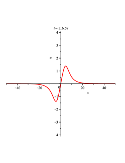
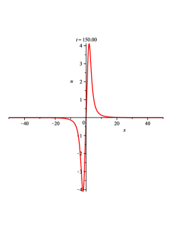
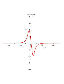
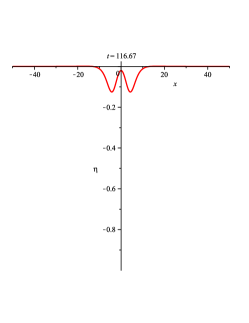
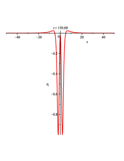
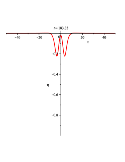
Figure 2: Snapshots of the solutions of the KB equation (94), (96) for three values of $t$. The first panel is before, the third panel is after the blowup.

The next case is a solution with $N=2$ discrete eigenvalues. Due to (20) there are the following situations:

(i) Both eigenvalues are on the imaginary axis: $\lambda_{1}=i\nu_{1}$, $\lambda_{2}=i\nu_{2}$ for some real and positive $\nu_{1}$ and $\nu_{2}$;

(ii) $\lambda_{2}=-\bar{\lambda}_{1}$, $R_{2}(\sigma)=\bar{R}_{1}(-\sigma)$. For the (ii) case from (8) we have

$$\underline{\psi}(x;\lambda,\sigma)\!\! = \!\!1\!+\!ie^{2i\sigma\omega_{+}}\left[\frac{R_{1}(\sigma)e^{2i\lambda_{1}x}\underline{\bar{\psi}}(x,\bar{\lambda}_{1},\sigma)}{\lambda-\lambda_{1}}\!+\!\frac{\bar{R}_{1}(\!-\!\sigma)e^{\!-\!2i\bar{\lambda}_{1}x}\underline{\psi}(x,\bar{\lambda}_{1},\!-\!\sigma)}{\lambda+\bar{\lambda}_{1}}\right],$$ (97)

From (97) we obtain a linear system of four equations for the quantities $\underline{\psi}(x,\bar{\lambda}_{1},\pm\sigma)$ and their complex conjugates by writing (97) for $\lambda=\bar{\lambda}_{1}$, the same with $\sigma$ replaced by $-\sigma$ and their complex conjugates.

The case with $N>2$ eigenvalues is always a combination between (i) and (ii) - in general it involves eigenvalues on the imaginary avis as well as conjugate couples $\lambda_{k}$ and $-\bar{\lambda}_{k}$.

10 Conclusions

We have outlined the inverse scattering for the spectral problems of the form (8) with real functions in the potential, which necesitates the $\mathbb{Z}_{2}$ reduction (20). The soliton solution in the case of a single pole of the eigenfunction does not have the form of a travelling wave and develops singularities with time. This solution is probably not relevant for the theory of water waves. There is another feature of this type of equations which points in the direction that the purely soliton solutions are probably not the ones which are observed in the context of water waves. Indeed, since $\eta$ is the deviation from the equilibrium surface, then one expects that its space-average value is zero, $\int_{-\infty}^{\infty}\eta(x,t)\text{d}x=0$. However, the trace identities which can be derived easily (see e.g. [23]) for the $N$-soliton solution of the KB equation lead to the following result:

$$\int_{-\infty}^{\infty}\eta(x,t)\text{d}x=\frac{1}{4}\int_{-\infty}^{\infty}(u^{2}+4w)\text{d}x=-4\sum_{k=1}^{N}\text{Im}\lambda_{k}.$$

By assumption $\text{Im}\lambda_{k}>0$ since $\lambda_{k}$ are in the upper half complex plane. Thus, we have the following ’mostly negative’ result for the $N$-soliton solution:

$$\int_{-\infty}^{\infty}\eta(x,t)\text{d}x<0.$$

This results indicates that the water wave solutions are related only to the continuous spectrum and are therefore unstable. This agrees with the fact that the travelling wave solutions to the Euler’s equation with zero surface tension are unstable.

11 Acknowledgments

The authors are indebted to Prof. V.S. Gerdjikov for many valuable discussions. This material is based upon works supported by the Science Foundation Ireland (SFI), under Grant No. 09/RFP/MTH2144.

References

• [1] M.J. Ablowitz and H. Segur, Solitons and the Inverse Scattering Transform, SIAM: Philadelphia, 1981.
• [2] M. Antonowicz and A. P. Fordy, ”Factorisation of energy dependent Schrödinger operators: Miura maps and modified systems,” Comm. Math. Phys., 124, 465–486 (1989).
• [3] M. Antonowicz, A. P. Fordy and Q.P. Liu, Energy-dependent third-order Lax operators, Nonlinearity 4 (1991) 669–684.
• [4] Borisov A B, Pavlov M V and Zykov S A, Proliferation scheme for the Kaup-Boussinesq system, Physica D 152/153 (2001) 104–9.
• [5] A. Constantin, Nonlinear Water Waves with Applications to Wave-Current Interactions and Tsunamis, SIAM: Philadelphia, 2011.
• [6] A. Constantin, R. Ivanov, On an integrable two-component Camassa-Holm shallow water system, Physics Letters A, 372 (2008), 7129–7132.
• [7] G.A. El, R.H.J. Grimshaw, M.V. Pavlov, Integrable shallow-water equations and undular bores, Stud. Appl. Math. 106 (2001) 157–186.
• [8] G.A. El, R.H.J. Grimshaw, A. M. Kamchatnov, Wave Breaking and the Generation of Undular Bores in an Integrable Shallow Water System, Studies in Applied Mathematics, Volume 114, Issue 4, pages 395–411, May 2005.
• [9] L.D. Faddeev and L.A. Takhtadjan, Hamiltonian approach in the theory of solitons, (Springer Verlag, Berlin, 1987).
• [10] V.S. Gerdjikov, G. Vilasi and A.B. Yanovski, Integrable Hamiltonian hierarchies. Spectral and geometric methods. Lecture Notes in Physics, 748. Springer-Verlag, Berlin, 2008.
• [11] R. H. J. Grimshaw, M. V. Pavlov, Integrable Shallow-Water Equations and Undular Bores, Studies in Applied Mathematics, Volume 106, Issue 2, pages 157–186, February 2001.
• [12] D. Holm and R. Ivanov, Two-component CH system: Inverse Scattering, Peakons and Geometry, Inverse Problems 27 (2011) 045013; arXiv:1009.5374v1 [nlin.SI].
• [13] D.D. Holm, T. Schmah and C. Stoica, Geometric Mechanics and Symmetry, Oxford University Press: Oxford, 2009.
• [14] R. Ivanov, Extended Camassa-Holm hierarchy and conserved quantities, Zeitschrift für Naturforschung, 61a (2006) 133–138, nlin.SI/0601066.
• [15] R. Ivanov, Two component integrable systems modelling shallow water waves: the constant vorticity case, Wave Motion 46 (2009), 389–396; arXiv:0906.0780
• [16] M. Jaulent, On an inverse scattering problem with an energy dependent potential, Ann. Inst. H. Poincaré Sect. A 17 (1972), 363–378.
• [17] Jaulent M. and Jean C. The inverse $s$-wave scattering problem for a class of potentials depending on energy. Comm. Math. Phys. 28 (1972) 177–220.
• [18] M. Jaulent and C. Jean, The inverse problem for the one-dimensional Schrödinger operator with an energy dependent potential. I, Ann. Inst. H. Poincaré Sect. A, 25 (1976), no. 2, 105–118; II, 119–137.
• [19] M. Jaulent and C. Jean, A Schrödinger inverse scattering problem with a spectral dependence in the potential, Lett. Math. Phys. 5 (1981) 183–190.
• [20] R. S. Johnson, A modern introduction to the mathematical theory of water waves, Cambridge University Press, Cambridge, 1997.
• [21] A.M. Kamchatnov, R.A. Kraenkel and B.A. Umarov, Asymptotic soliton train solutions of Kaup Boussinesq equations, Wave Motion 38 (2003) 355–365.
• [22] D.J. Kaup, A higher-order water-wave equation and the method for solving it, Progr. Theor. Phys. 54 (1975) 396–408.
• [23] A. Laptev, R. Shterenberg and V. Sukhanov, Inverse Spectral Problems for Schrödinger Operators with Energy Depending Potentials, Centre de Recherches Mathématiques CRM Proceedings and Lecture Notes, Volume 42, 2007.
• [24] V.B. Matveev and M.I. Yavor, Almost periodical solutions of nonlinear hydrodynamic equation of Kaup, Ann. Inst. H. Poincaré, Sect. A 31, 25–41 (1979).
• [25] A.V. Mikhailov, The reduction problem and the inverse scattering method, Physica D 3, n. 1–2 (1981) 73–117.
• [26] A.C. Newell, Solitons in Mathematical Physics, SIAM: Philadelphia, 1985.
• [27] M.V. Pavlov, Integrable Systems and Metrics of Constant Curvature, Journal of Nonlinear Mathematical Physics (2001) Volume: 9, Issue: Supplement 1, Pages: 173–191.
• [28] P. Popivanov, A. Slavova, Nonlinear waves. An Introduction, ISAAC series on Analysis, Applications and Comutation, vol.4, World Scientific, 2011.
• [29] Sattinger, D. H. and Szmigielski, J. A Riemann-Hilbert problem for an energy dependent Schrödinger operator. Inverse Problems 12 (1996) 1003–1025.
• [30] G. B. Whitham, Linear and nonlinear waves, J. Wiley & Sons Inc. (1999).
• [31] V.E. Zakharov, S.V. Manakov, S.P. Novikov and L.P. Pitaevskii, Theory of solitons: the inverse scattering method, (Plenum, New York, 1984).