Mott Insulator to Superfluid Phase Transition in Bravais Lattices via the Jaynes-Cummings-Hubbard Model

Abstract

The Properties of the Mott insulator to superfluid phase transition are obtained through the fermionic approximation in the Jaynes-Cummings-Hubbard model on linear, square, SC, FCC, and BCC Bravais lattices, For varying excitation number and atom-cavity frequency detuning. We find that the Mott lobes and the critical hopping are not scalable only for the FCC lattice. At the large excitation number regime, the critical hopping is scalable for all the lattices and it does not depend on the detuning.

1 Introduction

Cold-atom systems have been regarded as efficient simulators of quantum many-body physics BDZ ; JSGM due to its ease of controllability. Research involving ultracold bosonic systems has brought lot of interest in the subject AMC1 ; MOTT . Experiments with optical lattices in three dimensions have revealed the superfluid-Mott insulator (MI-SF) phase transition MG . Such phenomena have been studied in the frameworkof the Jaynes-Cummings-Hubbard Model (JCHM) Na1 ; Na2 ; NPA ; HASP .

The JCHM has been a widely used tool for the investigation of many-body systems describing the interplay between the atom-cavity coupling and the inter-cavity hopping of photons SB . In the absence of the hopping term, the model reduces to the Jaynes-Cummings Model JC ; EPJ1 which can be exactly solved within the Rotating Wave Approximation. When the hopping term is non-zero the solution becomes non trivial. The difficulty to find analytical solutions for the model has forced researchers to resort to approximation or numerical methods for dealing with such problems FWG . Recently, Mering et al. AMPK have proposed an approach in which spin operators are mapped to the fermionic ones, hence allowing the application of a Fourier transform that decouples the Hamiltonian into independent ones, which are associated to each momentum value. The great advantage of this method is the simplicity in which physical quantities are found, such as the energies and the chemical potential. The approach presented by Mering et al. includes all classes of Bravais structures. However, they only derived the results for one-dimensional lattices.

Despite the experiments involving optical structures in three dimensions, only a few theoretical results regarding these lattices in dimensions greater than one is available in the current literature EPJ2 . It lacks a systematic presentation of the phase diagram of typical Bravais lattices. This is the purpose of the present paper. Here, we investigate the JCHM for different Bravais lattices in one, two and three dimensions and analyse the influence of the topology on the MI-SF phase transition. We use the approach introduced by Mering et al. AMPK .

The paper is organized as follows. In Section II we introduce the JCHM. In Section III we present the fermionic approximation. Results are presented in Section IV. Finally, IN Section V, we summarize our main results and conclusions.

2 Jaynes-Cummings-Hubbard Model

The JCHM hamiltonian for a lattice of $L$ atoms is given by ($\hbar=1$)

$$\hat{H} =\omega \sum_{j}\hat{a}_{j}^{\dagger}\hat{a}_{j}+\epsilon\sum_{j}\hat{\sigma}_{j}^{+}\hat{\sigma}_{j}^{-}+g\sum_{j}(\hat{a}_{j}^{\dagger}\hat{\sigma}_{j}^{-}+\hat{a}_{j}\hat{\sigma}_{j}^{+})$$ (1)

$$-t\sum_{\langle ij\rangle}(\hat{a}_{i}^{\dagger}\hat{a}_{j}+\hat{a}_{j}^{\dagger}\hat{a}_{i}),$$

where $\hat{\sigma}^{\pm}=\hat{\sigma}_{x}\pm i\hat{\sigma}_{y}$ and $\hat{\sigma}_{x,y,z}$ are the usual Pauli matrices, $\hat{a}_{j}$ ($\hat{a}^{\dagger}_{j}$) is the annihilation (creation) operator of the light mode at the $j$th atom, $\omega$ is the light mode frequency, and $\epsilon$ the atomic transition frequency. The light-atom coupling is represented by $g$, $t$ is the hopping integral, and $\langle ij\rangle$ denotes pairs of nearest-neighbour atoms on the lattice.

When $t=0$, the Hamiltonian (1) is decoupled into $L$ independent Jaynes-Cummings model Hamiltonians. In this case the system has well-known eigenstates CNA . For $t\neq 0$, the atoms becomes coupled thus increasing the complexity of the solution, Since we can not write the eigenstates of the whole system as a direct product of single-cavity eigenstates. As discussed in the introduction, an appropriate approach is the fermionic approximation recently introduced by Mering et al. AMPK .

3 The Fermionic Approximation

The fermionic approximation consists in replacing the spin operators by fermionic ones, i.e., $\hat{\sigma}^{+}$ ($\hat{\sigma}^{-}$) IS replaced by $\hat{c}^{\dagger}$ ($\hat{c}$). In this framework, we can rewrite Hamiltonian (1) as

$$\hat{H} = \omega\sum_{j}\hat{a}_{j}^{\dagger}\hat{a}_{j}+\epsilon\sum_{j}\hat{c}_{j}^{\dagger}\hat{c}_{j}+g\sum_{j}(\hat{a}_{j}^{\dagger}\hat{c}_{j}+\hat{a}_{j}\hat{c}_{j}^{\dagger})$$ (2)

$$-t\sum_{\langle ij\rangle}(\hat{a}_{i}^{\dagger}\hat{a}_{j}+\hat{a}_{j}^{\dagger}\hat{a}_{i}).$$

This approximation allows to solve the model exactly, by means of a Fourier transformation. For $t=0$, spin and fermionic operators are equivalent and then the approximation becomes exact. Therefore, for small values of $t$ this approach turns out to be very accurate when dealing with the JCHM AMPK .

Now we apply a Fourier transform to the fermionic and bosonic operators as

$$\hat{a}_{j}=\frac{1}{\sqrt{L}}\sum_{\vec{k}}e^{-2\pi i\frac{\vec{k}\vec{R}_{j}}{L}}\hat{a}_{\vec{k}},\\ \hat{c}_{j}=\frac{1}{\sqrt{L}}\sum_{\vec{k}}e^{-2\pi i\frac{\vec{k}\vec{R}_{j}}{L}}\hat{c}_{\vec{k}},$$ (3)

then the Hamiltonian can be written as

$$\hat{H}=\sum_{\vec{k}}\left[\omega_{\vec{k}}\hat{a}_{\vec{k}}^{\dagger}\hat{a}_{\vec{k}}+g(\hat{a}_{\vec{k}}^{\dagger}\hat{c}_{\vec{k}}+\hat{a}_{\vec{k}}\hat{c}_{\vec{k}}^{\dagger})+\epsilon\hat{c}_{\vec{k}}^{\dagger}\hat{c}_{\vec{k}}\right],$$ (4)

where $\omega_{\vec{k}}=\omega$-$\nu_{\vec{k}}$ and $\nu_{\vec{k}}$ is the dispersion relation of the Bravais lattice.

The Hamiltonian (4) corresponds to a sum of $L$ independent Hamiltonians $\hat{H}_{\vec{k}}$ ($\hat{H}=\sum_{\vec{k}}\hat{H}_{\vec{k}}$), where each of them is associated with a particular momentum $\vec{k}$. The ground-state energy of $\hat{H}_{\vec{k}}$ is given by

$$E^{n_{\vec{k}}}_{\vec{k}} = (1-\delta_{n_{\vec{k}}0})\left[n_{\vec{k}}\omega_{\vec{k}}+\frac{\Delta+\nu_{\vec{k}}}{2}+\right.$$

$$\left.-\frac{1}{2}\sqrt{(\Delta+\nu_{\vec{k}})^{2}+4n_{\vec{k}}g^{2}}\right],$$ (5)

where the superscript denotes the excitation number and $\Delta\equiv\epsilon-\omega$ is the detuning between atomic trantition and light frequencies. Notice that $\hat{n}_{\vec{k}}$ commutes with $\hat{H}_{\vec{k}}$. For a total excitation number $N$ ($N=\sum_{\vec{k}}n_{\vec{k}}$) we have a particular configuration $\{n_{\vec{k_{1}}},n_{\vec{k_{2}}},n_{\vec{k_{3}}},...\}$ that minimizes the total ground-state energy, $\sum_{\vec{k}}E^{n_{\vec{k}}}_{\vec{k}}$. For $t\ll 1$, it is easy to see that this configuration is $\{n,n,n,...\}$ corresponding to the Mott insulator state. By increasing $t$, a quantum phase transition takes phace and the system is driven to a superfluid state. Since $n$ is constant, the phase boundaries of the Mott lobes are $n$ dependent. Thus, the $n$th Mott lobe is obtained through an analysis of the particles chemical potential, $\mu^{+}=E^{n+1}_{\vec{k}^{\prime}}-E^{n}_{\vec{k}^{\prime}}$, and the hole one, $\mu^{-}=E^{n}_{\vec{k}}-E^{n-1}_{\vec{k}}$ AMPK ; GAS , where $\vec{k}^{\prime}$ and $\vec{k}$ are, respectively, the values ​​that minimize and maximize these potentials. For $\mu^{+}=\mu^{-}$, the Mott lobe is closed at the critical hopping, $t_{c}$, hence describing the MI-SF transition.

4 Results

In order to analyse the influence of Bravais lattices topology on the MI-SF transition, we study the one-dimensional (1D), square (SQ), simple cubic (SC), body-centered cubic (BCC) and face-centered cubic (FCC) lattices. The dispersion relations $\nu_{\vec{k}}$ are, respectively, given by kitel

$$\nu_{k}^{(1D)}=-2t\cos(ka)$$ (6)

$$\nu_{k_{x},k_{y}}^{(SQ)}=-2t[\cos(k_{x}a)+\cos(k_{y}a)]$$ (7)

$$\nu_{k_{x},k_{y},k_{z}}^{(SC)}=-2t[\cos(k_{x}a)+\cos(k_{y}a)+\cos(k_{z}a)]$$ (8)

$$\nu_{k_{x},k_{y},k_{z}}^{(BCC)}=-8t[\cos(k_{x}a)\cos(k_{y}a)\cos(k_{z}a)]$$ (9)

and

$$\nu_{k_{x},k_{y},k_{z}}^{(FCC)} = -4t[\cos(k_{x}a)\cos(k_{y}a)+\cos(k_{x}a)\cos(k_{z}a)+$$

$$\cos(k_{y}a)\cos(k_{z}a)],$$ (10)

where $a$ is the lattice constant. For each structure we found the momentum vectors that maximizes the hole chemical potentials and minimizes the particle ones in order to obtain $\mu^{-}$, $\mu^{+}$, and consequently the Mott phase boundary.

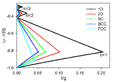
Figure 1: First three Mott lobes for different lattices. Inside the lobes we have a Mott insulator state, while outside the system is in a superfluid state.

Figure 1 shows the first three Mott lobes for $\omega/g=1$ and $\Delta=0$, for the considered lattices. We see that as the number of lattice neighbors increases, the MI phase region decreases. This result is expected since the probability of ohoton tunneling increases for higher number of nearest-neighbors. We observe that for $d$-dimensional hypercubic lattices the lobes can be rescaled by $t_{d}=t/d$ causing the collapse into a single curve. The shape of the Mott lobes are equal for bipartite lattices, where a bipartite structure is such one that we can decompose into two substructures, with all nearest-neighbour sites shared between each other. The FCC lattice is non-bipartite, Hence displaying a different behaviour. Thus we propose to make a detailed comparative analysis between the FCC and SC lattices representing, respectively, the non-bipartite and bipartite classes.

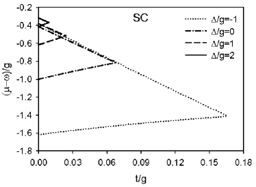
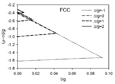
Figure 2: Mott lobe for $n=1$ and typical values of detuning for (a) SC and (b) FCC lattices.

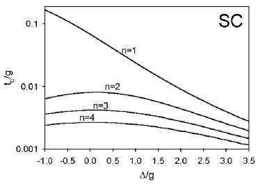
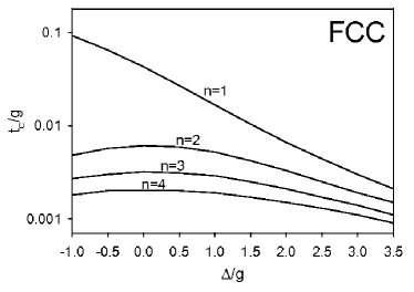
Figure 3: Relationship between critical hopping and detuning on the (a) SC and (b) FCC lattices for varying excitation number.

The first Mott lobe ($n=1$) on the SC and FCC lattice is show in figure 2 for typical detuning values. We see that both lattices have a similar MI-SF phase transition frame. However, the FCC always has a smaller MI phase region. For both lattices, the MI phase region decreases for increasing detuning. Figure 3 shows the critical hopping $t_{c}$ as a function of the detuning. While at the first lobe, $t_{c}$ decreases when $\Delta$ increases, in the other lobes ($n>1$) we observe that the critical hopping reaches a maximum at $\Delta=\Delta_{m}$. For this particular detuning value, when $n$ increases the critical hopping decreases, as predicted in AMPK . This behavior is present in both structures. Figure 4 shows the critical hopping as a function of $n$ for $\Delta=0$. The properties expressed by both lattices are again qualitatively equivalent where there is only one gap between the two curves. Figure 5 presents the detuning values corresponding to the maximal critical hopping as a function of $n$. We can observe that, except for the $n=1$ case, where the $t_{c}$ maximum is associated with the detuning minimum, The critical hopping correspondent detuning is approximately null.

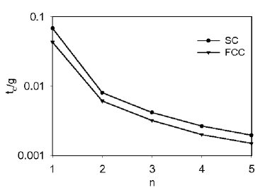
Figure 4: Critical hopping for the SC and FCC lattices in terms of $n$ for null detuning.

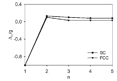
Figure 5: Detuning versus $n$ for maximal critical hopping on the SC and FCC lattices.

By performing an asymptotic approach to large excitation number, $n\gg 1$, we can find the dominant term of the critical hopping which is given by

$$t_{c}=\frac{g}{16\tilde{d}n^{3/2}}+{\cal O}(n^{-3}),$$ (11)

where we obtain $\tilde{d}=4$ for the FCC and BCC lattices where it corresponds to the hypercubic lattices dimentions, i. e., 1 for linear, 2 for square, and 3 for the SC lattice. It is important to emphasize that at the large-$n$ regime, the detuning and the topology class (bipartite or non-bipartite) influence on the critical hopping $t_{c}$ is suppressed. Figure 6 confirms the prediction of the equation (11). It shows that the exact results are in excellent agreement with the asymptotic ones for $n>4$.

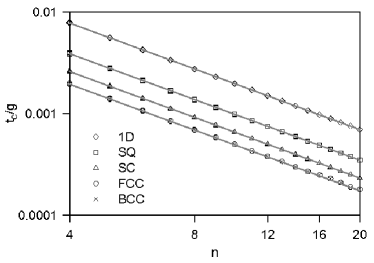
Figure 6: Critical hopping versus $n$ for various lattices at the large $n$ regime. The symbols are related to numerically obtained results for $\Delta/g=-0.5,0,$ and $0.5$, where each detuning value produces the same result with errors smaller than the symbol size. The solid line represents the asymptotic analytical result given by means of equation (11).

5 Conclusions

We have studied the properties of the MI-SF phase transition for the Jaynes-Cummings-Hubbard model over several Bravais lattices by means of the fermionic approximation. We find that the transition parameters of hypercubic lattices are scalable, except for the FCC lattice, since it is non-bipartite. The Mott lobes for the SC and FCC lattices show a similar detuning dependence having only a quantitative difference which is suppressed as the detuning increases. An analogous feature is observed in $t_{c}$ vs. $n$ for null delta and in $\Delta_{m}$ vs. $n$ where treir quantitative difference tends to be smaller as $n$ increases. Furthermore, we observed that not only the number of neighbors influences the MI-SF phase transition but also does the lattice topology.

The FCC lattice shows a behavior quantitatively different and non-scalable from bipartite lattices. On the other hand, asymptotic results for large excitation number indicate an universality on $t_{c}$ because it obeys a power law in $n$ which does not depend on $\Delta$ and topology associated parameter can be rescaled for different classes through a multiplication of $t_{c}$ by an effective parameter that corresponds to the dimension, for hypercubic, and to 4, for BCC and FCC lattices.

References

- (1) I. Bloch, J. Dalibard and W. Zwerger Rev. Mod. Phys. 80 885 (2008)
- (2) R. Jordens, N. Strohmaier, K. Günter, H. Moritz and T. Esslinger, Nature 455 204-207 (2008)
- (3) S. Valencia and A.M.C. Souza, Eur. Phys. J. B 85, 161 (2012)
- (4) M. Greiner et. al., Nature (London) 415 39 (2002)
- (5) M. Greiner, O. Mandel, T. Esslinger, T. W. Hansch and I. Bloch Nature 415, 39-44 (2002)
- (6) M. J. Hartmann, F. G. S. L. Brandão and M. B. Plenio, Nat. Phys. 2, 849 (2006)
- (7) A. D. Greentree, C. Tahan, J. H. Cole and L. C. L. Hollenberg, Nat. Phys. 2, 856 (2006)
- (8) C. Nietner and A. Pelste Phys. Rev. A 85 043831 (2012)
- (9) M. Hohenadler, M. Aichhorn, S. Schmidt and L. Pollet Phys. Rev. A 84 041608 (2011)
- (10) S. Schmidt and G. Blatter Phys. Rev. Lett. 103 086403 (2009)
- (11) E.T. Jaynes, F.W. Cummings, Proc. IEEE 51, 89 (1963)
- (12) M. Bina, Eur. Phys. J. Special Topics 203, 163-183 (2012)
- (13) M. P. A. Fisher, P. B. Weichman, G. Grinstein and D, S. Fisher Phys. Rev. B 40 546 (1989)
- (14) A. Mering, M. Fleischhauer, P. A. Ivanov and K. Singer Phys. Rev. A 80 053821 (2009)
- (15) S. Ghanbari1, P. B. Blakie, P. Hannaford and T. D. Kieu, Eur. Phys. J. B 70, 305-310 (2009)
- (16) C. Nietner and A. Pelster, Phys. Rev. A 85, 043831 (2012)
- (17) C. B. Gomes, F. A. G. Almeida and A. M. C. Souza, arXiv:1209.5321v1 (2012)
- (18) C. Kittel, Introduction to Solid State Physics, Wiley, 8th Edition (2004)