Inference of seasonal long-memory aggregate time series

Abstract

Time-series data with regular and/or seasonal long-memory are often aggregated before analysis. Often, the aggregation scale is large enough to remove any short-memory components of the underlying process but too short to eliminate seasonal patterns of much longer periods. In this paper, we investigate the limiting correlation structure of aggregate time series within an intermediate asymptotic framework that attempts to capture the aforementioned sampling scheme. In particular, we study the autocorrelation structure and the spectral density function of aggregates from a discrete-time process. The underlying discrete-time process is assumed to be a stationary Seasonal AutoRegressive Fractionally Integrated Moving-Average (SARFIMA) process, after suitable number of differencing if necessary, and the seasonal periods of the underlying process are multiples of the aggregation size. We derive the limit of the normalized spectral density function of the aggregates, with increasing aggregation. The limiting aggregate (seasonal) long-memory model may then be useful for analyzing aggregate time-series data, which can be estimated by maximizing the Whittle likelihood. We prove that the maximum Whittle likelihood estimator (spectral maximum likelihood estimator) is consistent and asymptotically normal, and study its finite-sample properties through simulation. The efficacy of the proposed approach is illustrated by a real-life internet traffic example.

and

1 Introduction

Data are often aggregated before analysis, for example, 1-minute data aggregated into half-hourly data or daily data aggregated into monthly data. Aggregation of data may be carried out for ease of interpretation on a scale that is of interest, for example, policy makers and/or the public are more interested in monthly unemployment rate than daily unemployment rate. On the other hand, data may be naturally aggregated, for example, tree-ring data, which are often hard to disaggregate. On a fine sampling scale, many time series are of long memory in the sense that their spectral density functions admit a pole at the zero frequency. A popular class of discrete time long memory processes are autoregressive fractionally integrated moving average (ARFIMA) models (see Granger and Joyeux [6], Hosking [7]). Man and Tiao [11] and Tsai and Chan [18] showed that temporal aggregation preserves the long-memory parameter of the underlying ARFIMA process. Ohanissian, Russell and Tsay [13] made use of this property in developing a test for long-memory. Furthermore, as the extent of aggregation increases to infinity, the limiting model retains the long-memory parameter of the original process, whereas the short-memory components vanish.

In practice, the underlying process may admit seasonal long memory in that its spectral density function may have poles at certain non-zero frequencies. Such data may be modeled as some Seasonal Auto-Regressive Fractionally Integrated Moving-Average (SARFIMA) process, see Section 2. If the aggregation interval is much larger than the largest seasonal period, aggregation will intuitively merge the seasonal long-memory components with the regular long-memory component and eliminate the regular or seasonal short-memory components of the raw data. For example, within the framework of ARIMA models, Wei [19] showed that aggregation removes seasonality if the frequency of aggregation is larger than or the same as the seasonal frequency.

On the other hand, if the aggregation interval is large but is just some fraction of the seasonal periods of the original data, the aggregates may be expected to keep the seasonal short- and long-memory pattern, albeit with different periods. For many data, the latter scenario may be more relevant for analysis. For example, aggregating 1-minute data into half-hourly data may remove the short memory component on the minute scale but the daily or monthly correlation pattern of the raw data may persist in the aggregates.

Here, our purposes are twofold. First, we study the intermediate asymptotics of aggregating a SARFIMA process. In particular, we derive the limiting (normalized) spectral density function of an aggregated SARFIMA process via the asymptotic framework where the seasonal periods of the SARFIMA model are multiples of the aggregation interval and the aggregation interval is large. While the original time series is assumed to be a SARFIMA process, the limiting result is robust to the exact form of the short-memory and the regular long-memory components. The limiting spectral density functions then define a class of models suitable for analyzing aggregate time series that may have regular or seasonal long-memory and short-memory components. Second, we derive the large-sample properties of the spectral maximum likelihood estimator of the limiting aggregate SARFIMA model, obtained by maximizing the Whittle likelihood.

The rest of the paper is organized as follows. The SARFIMA model is reviewed in Section 2. In Section 3, we derive the limiting spectral density function of an aggregate SARFIMA process, under the intermediate asymptotic framework. Spectral maximum likelihood estimation of the limiting aggregate SARFIMA model and its large-sample properties are discussed in Section 4. We compare the empirical performance of the spectral maximum likelihood estimator of the limiting model with that of the SARFIMA model by Monte Carlo studies in Section 5. The simulation results suggest that fitting the limiting model to the aggregate data generally reduces the bias in some long-memory parameters than simply fitting a SARFIMA model. We illustrate the use of the limiting aggregate SARFIMA model and its possible gains in long-term forecasts with a real application in Section 6. We conclude in Section 7. All proofs are collected in the appendix of Chan and Tsai [5].

2 Seasonal autoregressive fractionally integrated moving average models

We now briefly review the SARFIMA model which is widely useful in scientific analysis; see Porter-Hudak [16], Ray [17], Montanari, Rosso and Taqqu [12], Palma and Chan [15], Bisognin and Lopes [2] and Lopes [10]. Let $\{Y_{t},t=0,\pm 1,\pm 2,\ldots\}$ be a seasonal autoregressive fractionally integrated moving average (SARFIMA) model with multiple periods $s_{1},\ldots,s_{c}$

$$\phi(B)(1-B)^{d}\prod_{i=1}^{c}\Phi_{i}(B^{s_{i}})(1-B^{s_{i}})^{D_{i}}Y_{t}=\theta(B)\prod_{i=1}^{c}\Theta_{i}(B^{s_{i}})\varepsilon_{t},$$ (1)

where $d$ and $D_{i},i=1,\ldots,c$, are real numbers, $s_{c}>s_{c-1}>\cdots>s_{1}>1$ are integers, $\{\varepsilon_{t}\}$ is an uncorrelated sequence of random variables with zero mean and common, finite variance $\sigma^{2}_{\varepsilon}>0$, $\phi(z)=1-\phi_{1}z-\cdots-\phi_{p}z^{p}$, $\theta(z)=1+\theta_{1}z+\cdots+\theta_{q}z^{q}$, and for $i=1,\ldots,c$, $\Phi_{i}(z)=1-\Phi_{i,1}z-\cdots-\Phi_{i,P_{i}}z^{P_{i}}$, $\Theta_{i}(z)=1+\Theta_{i,1}z+\cdots+\Theta_{i,Q_{i}}z^{Q_{i}}$, $B$ is the backward shift operator, and $(1-B)^{d}$ is defined by the binomial series expansion

$$(1-B)^{d}=\sum_{k=0}^{\infty}\frac{\Gamma(k-d)}{\Gamma(k+1)\Gamma(-d)}B^{k},$$

where $\Gamma(\cdot)$ is the gamma function. Stationarity of $\{Y_{t}\}$ requires $D_{i}<1/2$ for all $i$ and $d+\sum_{i=1}^{c}D_{i}<1/2$, see Palma and Bondon [14]. We assume that none of the roots of $\phi(\cdot)$ and $\Phi_{i}(\cdot),$ $i=1,\ldots,c$, match any roots of $\theta(\cdot)$ and $\Theta_{i}(\cdot),$ $i=1,\ldots,c$. Moreover, all roots of of the above polynomials are assumed to lie outside the unit circle. The conditions on the roots, the fractional orders $d$ and $D$’s ensure that $\{Y_{t}\}$ is stationary and the model is identifiable. It can be readily checked that the spectral density of $\{Y_{t}\}$ equals, for $-\uppi<\omega\leq\uppi$,

$$h(\omega) = \frac{\sigma^{2}}{2\uppi}\biggl{|}\frac{\theta(\exp(\mathrm{i}\omega))}{\phi(\exp(\mathrm{i}\omega))}\biggr{|}^{2}\biggl{|}2\sin\biggl{(}\frac{\omega}{2}\biggr{)}\biggr{|}^{-2\delta_{0}}\prod_{j=1}^{c}\biggl{|}\frac{\Theta_{j}(\exp(\mathrm{i}s_{j}\omega))}{\Phi_{j}(\exp(\mathrm{i}s_{j}\omega))}\biggr{|}^{2}$$

$${}\times\prod_{j=1}^{c}\prod_{k=1}^{\tau_{j}}\bigl{|}\bigl{(}\exp(\mathrm{i}\nu_{jk})-\exp(\mathrm{i}\omega)\bigr{)}\bigl{(}\exp(-\mathrm{i}\nu_{jk})-\exp(\mathrm{i}\omega)\bigr{)}\bigr{|}^{-2\delta_{jk}},$$

where $\delta_{0}=d+D_{1}+\cdots+D_{c}$; $\tau_{j}=[s_{j}/2]$, the greatest integer $\leq s_{j}/2$; $\nu_{jk}=2\pi k/s_{j}$, for $j=1,\ldots,c$, and $k=1,\ldots,\tau_{j}$; $\delta_{jk}=D_{j}$, for $k=1,\ldots,\tau_{j}-1$, $\delta_{j\tau_{j}}=D_{j}$ if $s_{j}=2\tau_{j}+1$, and $\delta_{j\tau_{j}}=D_{j}/2$ if $s_{j}=2\tau_{j}$. From (2), we see that, as $\omega\to 0$, the spectral density $f(\omega)=\mathrm{O}(|\omega|^{-2d-2D_{1}-\cdots-2D_{c}})$, whereas for $j=1,\ldots,c$, $k=1,\ldots,\tau_{j}$, as $\omega\to\nu_{jk}$, $f(\omega)=\mathrm{O}(|\omega-\nu_{jk}|^{-2D_{j}})$. Given our interest in long-memory processes, throughout this paper, the parameters $d$ and the $D_{j}$’s are restricted by the inequality constraints: $0\leq d+D_{1}+\cdots+D_{c}<1/2$, and $0\leq D_{j}<1/2$, for $j=1,\ldots,c$.

3 Aggregates of SARFIMA models

For non-stationary data, we assume that, after suitable regular and/or seasonal differencing, the data become stationary and follow some stationary SARFIMA model. Specifically, let $r$ and $R_{j}$, $j=1,\ldots,c$, be non-negative integers and $\{Y_{t},t=0,\pm 1,\pm 2,\ldots\}$ a time series such that $(1-B)^{r}(1-B^{s_{1}})^{R_{1}}\cdots(1-B^{s_{c}})^{R_{c}}Y_{t}$ is a stationary SARFIMA model defined by equation (1). Therefore, $\{Y_{t}\}$ satisfies the difference equation

$$\phi(B)(1-B)^{r+d}\prod_{j=1}^{c}\Phi_{j}(B^{s_{j}})(1-B^{s_{j}})^{R_{j}+D_{j}}Y_{t}=\theta(B)\prod_{j=1}^{c}\Theta_{j}(B^{s_{j}})\varepsilon_{t},$$ (3)

which is referred to as the $\operatorname{SARFIMA}(p,r+d,q)\times(P_{1},R_{1}+D_{1},Q_{1})_{s_{1}}\times\cdots\times(P_{c},R_{c}+D_{c},Q_{c})_{s_{c}}$ model.

Let $m\geq 2$ be an integer and $X_{T}^{m}=\sum_{k=m(T-1)+1}^{mT}Y_{k}$ be the nonoverlapping $m$-temporal aggregates of $\{Y_{t}\}$. Let $\nabla=1-B$ be the first difference operator, and $\nabla_{s}=1-B^{s}$ the lag-$s$ difference operator. Let $R=(r,R_{1},\ldots,R_{c})$, $\xi=(d;D_{j},j=1,\ldots,c;\Phi_{i,j},i=1,\ldots,c,j=1,\ldots,P_{i};\Theta_{i,j},i=1,\ldots,c,j=1,\ldots,Q_{i})$, and assume $s_{i}=mz_{i}$, $i=1,\ldots,c$, where the $z_{i}$’s are positive integers. Below we derive the spectral density of the aggregates, and the limit of the normalized spectral densities with increasing aggregation. The normalization that makes the spectral densities integrate to 1 is necessary because, without normalization, the variance of the aggregates generally increases to infinity with increasing aggregation.

Theorem 1.

Assume that $\{Y_{t}\}$ satisfies the difference equation defined by (3). [

• (a)] For $r\geq 0$, $R_{i}\geq 0$, $i=1,\ldots,c$, and $m=2h+1$, the spectral density function of $\{\nabla^{r}\nabla_{z_{1}}^{R_{1}}\cdots\nabla_{z_{c}}^{R_{c}}X_{T}^{m}\}$ is given by

  $$f_{\xi,R,m}(\omega) = \frac{1}{m}\biggl{|}2\sin\biggl{(}\frac{\omega}{2}\biggr{)}\biggr{|}^{2r+2}\prod_{j=1}^{c}\biggl{|}2\sin\biggl{(}\frac{z_{j}\omega}{2}\biggr{)}\biggr{|}^{-2D_{j}}\prod_{j=1}^{c}\biggl{|}\frac{\Theta_{j}(\exp(\mathrm{i}z_{j}\omega))}{\Phi_{j}(\exp(\mathrm{i}z_{j}\omega))}\biggr{|}^{2}$$

  $${}\times\sum_{k=-h}^{h}\biggl{|}2\sin\biggl{(}\frac{\omega+2k\uppi}{2m}\biggr{)}\biggr{|}^{-2r-2d-2}g\biggl{(}\frac{\omega+2k\uppi}{m}\biggr{)},$$

  where $g(\omega)=\sigma^{2}(2\uppi)^{-1}|\theta(\exp(\mathrm{i}\omega))|^{2}|\phi(\exp(\mathrm{i}\omega))|^{-2}$ and $-\uppi<\omega\leq\uppi$.

  If $m=2h$, the spectral density is given by equation (1) with the summation ranging from $-h+1$ to $h$ for $-\uppi<\omega\leq 0$ and from $-h$ to $h-1$ for $0<\omega\leq\uppi$.

• As $m\to\infty$, the normalized spectral density function of $\{\nabla^{r}\nabla_{z_{1}}^{R_{1}}\cdots\nabla_{z_{c}}^{R_{c}}X_{T}^{m}\}$ converges to $f_{\xi,R}(\omega)=K_{\xi,R}f^{*}_{\xi,R}(\omega)$, where

  $$f^{*}_{\xi,R}(\omega) = \biggl{|}\sin\biggl{(}\frac{\omega}{2}\biggr{)}\biggr{|}^{2r+2}\prod_{j=1}^{c}\biggl{|}\sin\biggl{(}\frac{z_{j}\omega}{2}\biggr{)}\biggr{|}^{-2D_{j}}$$

  $${}\times\prod_{j=1}^{c}\biggl{|}\frac{\Theta_{j}(\exp(\mathrm{i}z_{j}\omega))}{\Phi_{j}(\exp(\mathrm{i}z_{j}\omega))}\biggr{|}^{2}\sum_{k=-\infty}^{\infty}|\omega+2k\uppi|^{-2r-2d-2},$$

  where $K_{\xi,R}$ is the normalization constant ensuring that $\int_{-\uppi}^{\uppi}f_{\xi,R}(\omega)\,\mathrm{d}\omega=1$.

Remark 1.

The assumption that $s_{i}=mz_{i}$, for $i=1,\ldots,c$, and $m\to\infty$ in Theorem 1(b) should be interpreted as follows: the periodicities $s_{i}$’s are multiples of the aggregation size $m$, and the aggregation size is large. Consider two examples. Example (1): hourly data (that have a quarterly seasonality) are aggregated into monthly data, so $s=2160$, $m=720$, and $z=3$, and Example (2): half-hourly data (that have a weekly seasonality) are aggregated into daily data, so $s=336$, $m=48$, $z=7$.

Remark 2.

Note that $z_{c}>z_{c-1}>\cdots>z_{1}\geq 1$. For $j=1,\ldots,c$, $k=0,1,\ldots,[z_{j}/2]$, let $\omega_{jk}=\nu_{j(mk)}=2\uppi k/z_{j}$, then both $m^{-2r-2d-1}f_{\xi,R,m}$ and $f_{\xi,R}$ are of order$\mathrm{O}(|\omega|^{-2d-2D_{1}-\cdots-2D_{c}})$, for $\omega\to 0$, and of order $\mathrm{O}(|\omega-\omega_{jk}|^{-2D_{j}})$, for $\omega\to\omega_{jk}$, $j=1,\ldots,c$, $k=1,\ldots,[z_{j}/2]$. The above observations indicate that, if the periodicities $s_{i}$’s are multiples of the aggregation size $m$, then the aggregates and their limits preserve the long-memory and seasonal long-memory parameters of the underlying SARFIMA process, whereas the $z_{i}$’s become the periodicities of the aggregated series.

Remark 3.

If $z_{1}=1$, the corresponding seasonal long-memory component is confounded with the regular long-memory component for the limiting aggregate process. Hence, without loss of generality, we shall set $D_{1}=0$ if $z_{1}=1$ in applications.

Remark 4.

If $r=0$, then the limiting model of the aggregates of $\{Y_{t}\}$ is simply a $\operatorname{SARFIMA}(P_{1},R_{1}+D_{1},Q_{1})_{z_{1}}\times\cdots\times(P_{c},R_{c}+D_{c},Q_{c})_{z_{c}}$ process with fractional Gaussian noise as the driving noise process, where the self-similarity parameter (Hurst parameter) of the underlying fractional Gaussian process equals $H=d+1/2$. See Beran [1] for definition of the fractional Gaussian noise.

4 Spectral maximum likelihood estimator and its large sample properties

We are interested in applying the long-memory limiting aggregate process derived in Section 3 to data analysis. For this purpose, we assume (i) $0\leq d+D_{1}+\cdots+D_{c}<1/2$ and (ii) $0\leq D_{j}<1/2$ for $j=1,\ldots,c$. The limiting aggregate process is of long memory regularly or seasonally if either $0<d+D_{1}+\cdots+D_{c}<1/2$ or $0<D_{j}<1/2$ for some $j\in\{1,\ldots,c\}$. We also introduce the parameter $\sigma$ to account for the variance of the data. Furthermore, we assume $z_{j}$, $j=1,\ldots,c,$ are known. Consider a time series $\{Y_{i}\}_{i=1-\delta}^{N}$, where $\delta$ is a positive integer to be defined below, such that, conditional on $\{Y_{i}\}_{i=1-\delta}^{0}$, $\{\nabla^{r}\nabla_{z_{1}}^{R_{1}}\cdots\nabla_{z_{c}}^{R_{c}}Y_{i}\}_{i=1}^{N}$ is a stationary process with its spectral density defined by

$$f(\omega;\xi,R,\sigma^{2})=\sigma^{2}f^{*}(\omega;\xi,R),$$ (6)

where $f^{*}(\omega;\xi,R)$ is define in ((b)), $\delta=\max_{r}+\sum_{i=1}^{c}z_{i}\cdot\max_{R_{i}}$; $\max_{r}$ and $\max_{R_{i}}$, $i=1,\ldots,c$, are the largest possible values of $r$ and $R_{i}$, $i=1,\ldots,c$, respectively, which we will consider in simulation studies and real data analysis in Sections 5 and 6. That is, the spectral maximum likelihood estimators $\hat{r}$ and $\hat{R}_{i}$, $i=1,\ldots,c$, satisfy the conditions that $\hat{r}\in\{0,\ldots,\max_{r}\}$ and $\hat{R}_{i}\in\{0,\ldots,\max_{R_{i}}\}$, for $i=1,\ldots,c$.

It can be easily checked that, conditional on $\{Y_{i}\}_{i=1-\delta}^{0}$, the joint distributions of $\{\nabla^{r}\nabla_{z_{1}}^{R_{1}}\cdots\nabla_{z_{c}}^{R_{c}}Y_{i}\}_{i=1}^{N}$ and $\{Y_{i}\}_{i=1}^{N}$ are the same. Therefore, conditional on $\{Y_{i}\}_{i=1-\delta}^{0}$, the (negative) log-likelihood function of $\{Y_{i}\}$ can be approximated by the (negative) Whittle log-likelihood function (see Hosoya [8])

$$-\tilde{l}(\xi,R,\sigma^{2})=\sum_{j=1}^{T}\biggl{\{}\log f(\omega_{j};\xi,R,\sigma^{2})+\frac{I_{N}(\omega_{j};R)}{f(\omega_{j};\xi,R,\sigma^{2})}\biggr{\}},$$ (7)

where $\omega_{j}:=2\uppi j/N\in(0,\uppi)$ are the Fourier frequencies, $T$ is the largest integer $\leq(N-1)/2$, $I_{N}(\omega;R)=|\sum_{j=1}^{N}U_{j}(R)\exp(\mathrm{i}j\omega)|^{2}/(2\uppi N)$, and $U_{i}(R)=\nabla^{r}\nabla_{z_{1}}^{R_{1}}\cdots\nabla_{z_{c}}^{R_{c}}Y_{i}$, $i=1,\ldots,N$. In (7), the computation of $f(\omega_{j};\xi,R,\sigma^{2})$ requires evaluation of an infinite sum. Here, we adopt the method of Chambers [4] to approximate $f(\omega;\xi,R,\sigma^{2})$ by

$$\tilde{f}(\omega;\xi,R,\sigma^{2})$$

$$\quad=\sigma^{2}\biggl{|}\sin\biggl{(}\frac{\omega}{2}\biggr{)}\biggr{|}^{2r+2}\prod_{j=1}^{c}\biggl{|}\sin\biggl{(}\frac{z_{j}\omega}{2}\biggr{)}\biggr{|}^{-2D_{j}}\prod_{j=1}^{c}\biggl{|}\frac{\Theta_{j}(\exp(\mathrm{i}z_{j}\omega))}{\Phi_{j}(\exp(\mathrm{i}z_{j}\omega))}\biggr{|}^{2}h(\omega;\xi,R),$$

where $h(\omega;\xi,R)=\{2\uppi(2r+2d+1)\}^{-1}\{(2\uppi M-\omega)^{-2r-2d-1}+(2\uppi M+\omega)^{-2r-2d-1}\}+\sum_{k=-M}^{M}|\omega+2k\uppi|^{-2r-2d-2}$ for some large integer $M$. By routine analysis, it can be shown that, under the conditions stated in Theorem 2, the approximation error of $h(\omega;R,\xi)$ to the infinite sum is of order $\mathrm{O}(M^{-2r-2d-2})$. Also, the approximation error of the first partial derivative with respect to $d$ is of order $\mathrm{O}(M^{-2r-2d-1-\epsilon})$, for any positive $\epsilon$ less than 1. These error rates guarantee that if the truncation parameter $M$ increases with the sample size at a suitable rate, then the truncation has negligible effects on the asymptotic distribution of the estimator, see Theorem 2 below. Replacing $f(\omega_{j};\xi,R,\sigma^{2})$ by $\tilde{f}(\omega_{j};\xi,R,\sigma^{2})$ and letting $\tilde{g}(\omega_{j};\xi,R)=\tilde{f}(\omega_{j};\xi,R,\sigma^{2})/\sigma^{2}$, the (negative) Whittle log-likelihood function (7) now becomes

$$-\tilde{l}(\xi,R,\sigma^{2})=\sum_{j=1}^{T}\biggl{\{}\log\sigma^{2}+\log\tilde{g}(\omega_{j};\xi,R)+\frac{I_{N}(\omega_{j};R)}{\sigma^{2}\tilde{g}(\omega_{j};\xi,R)}\biggr{\}}.$$ (8)

Differentiating (8) with respect to $\sigma^{2}$ and equating to zero gives

$$\hat{\sigma}^{2}=\frac{1}{T}\sum_{j=1}^{T}\frac{I_{N}(\omega_{j};R)}{\tilde{g}(\omega_{j};\xi,R)}.$$ (9)

Substituting (9) into (8) yields the objective function

$$-\tilde{l}(\xi,R)=\sum_{j=1}^{T}\log\tilde{g}(\omega_{j};\xi,R)+T\log\Biggl{(}\sum_{j=1}^{T}\frac{I_{N}(\omega_{j};R)}{\tilde{g}(\omega_{j};\xi,R)}\Biggr{)}+C,$$ (10)

where $C=T-T\log T$. The objective function is minimized with respect to $\xi$ and $R$ to get the spectral maximum likelihood estimators $\hat{\xi}$ and $\hat{R}$; the estimator $\hat{\sigma}^{2}$ is then calculated by (9). Specifically, the spectral maximum likelihood estimators $\hat{\xi}$ and $\hat{R}$ are computed based on equation (10) using the following procedure (Recall that $0\leq D_{j}<1/2$, for $j=1,\ldots,c$, and $0\leq d+D_{1}+\cdots+D_{c}<1/2$). For each $\tilde{r}\in\{0,\ldots,\max_{r}\}$ and $R_{i}\in\{0,\ldots,\max_{R_{i}}\}$, for $i=1,\ldots,c$, we first find the local maximum likelihood estimator of $\xi$ in the range that $0\leq D_{j}<1/2$, $j=1,\ldots,c$, and $\tilde{r}\leq r+d+D_{1}+\cdots+D_{c}<\tilde{r}+1/2$. In our experiments, we let $\max_{r}=\max_{R_{1}}=\cdots=\max_{R_{c}}=2$. These local maximum likelihood estimators are then used to find the global maximum likelihood estimator of $\xi$ and $R=(r,R_{1},\ldots,R_{c})$.

For simplicity, let $\theta=(\xi,\sigma^{2})$, $\hat{\theta}=(\hat{\xi},\hat{\sigma}^{2})$ and $\hat{R}$ be the spectral maximum likelihood estimator that minimizes the (negative) Whittle log-likelihood function (8). Below, we derive the large-sample distribution of the spectral maximum likelihood estimator.

Theorem 2.

Let the data $Y=\{Y_{i}\}_{i=1}^{N}$ be such that $\{\nabla^{r}\nabla_{z_{1}}^{R_{1}}\cdots\nabla_{z_{c}}^{R_{c}}Y_{i}\}_{i=1}^{N}$ is sampled from a stationary Gaussian seasonal long-memory process with the spectral density given by (6). Let the spectral maximum likelihood estimator $\hat{\theta}\in\Theta$, a compact parameter space, and the true parameter $\theta_{0}$ be in the interior of the parameter space. Assume that each component of $R=(r,R_{1},\ldots,R_{c})$ is known to be between $0$ and some integer $K$. Let $r_{0}$ and $d_{0}$ be the true values of $r$ and $d$, and the truncation parameter $M$ increase with the sample size so that $M\to\infty$. Then the spectral maximum likelihood estimator $\hat{R}$ and $\hat{\theta}$ are consistent. Moreover, if $\sqrt{N}M^{-2r_{0}-2d_{0}-1}\to 0$ as $N\to\infty$, then $\sqrt{N}(\hat{\theta}-\theta_{0})$ converges in distribution to a normal random vector with mean 0 and covariance matrix $\Gamma(\theta_{0})^{-1}$ with

$$\Gamma(\theta)=\frac{1}{4\uppi}\int_{-\uppi}^{\uppi}(\bigtriangledown\log f(\omega;R,\theta))(\bigtriangledown\log f(\omega;R,\theta))^{\prime}\,\mathrm{d}\omega,$$ (11)

where $\bigtriangledown$ denotes the derivative operator with respect to $\theta$, and superscript ^′ denotes transpose.

5 Empirical comparison between the limiting model and the SARFIMA model

Given aggregation is finite in practice, fitting the limiting model (6) to aggregate data may result in bias, even though the bias vanishes with increasing aggregation. On the other hand, “to some extent, a discrete time series model is conditional on the time scale,” as remarked by a referee. So, it is pertinent to compare the empirical performance of the long-memory parameter estimators based on the proposed limiting model with those based on the SARFIMA model fitted to the aggregate data. As aggregation carries a signature in the long-memory data structure as spelt out in Theorem 1, fitting a SARFIMA model to aggregate data may result in even larger bias on the long-memory parameters than the limiting model. Here, we report some simulation results for clarifying the aforementioned issue. Consider the aggregated time series $\{Y_{i}\}_{i=1-\delta}^{N}$ such that $\{\nabla^{r}\nabla_{z}^{R}Y_{i}\}_{i=1}^{N}$ is a stationary process with its spectral density defined by

$$f(\omega;r,d,D,\sigma^{2}) = \sigma^{2}\biggl{|}\sin\biggl{(}\frac{\omega}{2}\biggr{)}\biggr{|}^{2r+2}\biggl{|}\sin\biggl{(}\frac{z\omega}{2}\biggr{)}\biggr{|}^{-2D}$$

$${}\times\sum_{k=-h}^{h-1}\biggl{|}(2m)\sin\biggl{(}\frac{\omega+2k\uppi}{2m}\biggr{)}\biggr{|}^{-2r-2d-2}g\biggl{(}\frac{\omega+2k\uppi}{m}\biggr{)},$$

where $g(\omega)=|\phi(\exp(\mathrm{i}\omega))|^{-2}$, $\phi(x)=1-\phi_{1}x$, $\delta=\max_{r}+\max_{R}z$, and $0<\omega<\uppi$. For $-\uppi<\omega\leq 0$, $f(\omega;r,d,D,\sigma^{2})=f(-\omega;r,d,D,\sigma^{2})$. We consider $\sigma=2$, $z=10$, and $r=R=0$. The true values of $(d,D)$ are (i) ($-0.1,0.3$) and (ii) ($0.2,0.25$), whereas those of the other parameters are given in Table 5. The sample sizes considered are $N=512$ and $N=1024$. We tried a range of $\operatorname{AR}(1)$ coefficient $\phi_{1}$: $-0.9,-0.5,0.0,0.5$, and $0.9$. The aggregation size $m$ are set to be $60$, $240$, and $720$, corresponding to the cases that minutely data are aggregated over one hour, four hours, and half a day, respectively. To each aggregated time series simulated from model (5), we fitted (i) the limiting aggregate model, and (ii) the SARFIMA model. The averages and the standard deviations, as well as the asymptotic standard errors, of 1000 replicates of the estimators for (i) $(d,D)=(-0.1,0.3)$ and (ii) $(d,D)=(0.2,0.25)$ are summarized in Tables 5 and 5, respectively. Note that the estimates of $r$ and $R$ equal zero for all simulations.

=Averages (standard deviations) of 1000 simulations of the spectral maximum likelihood estimators of the parameters $d$, and $D$ by fitting the limiting aggregate model (6) and the SARFIMA model (2), respectively, to aggregate data generated according to (5), with $(d,D)=(-0.1,0.3)$. The asymptotic standard errors for the estimators of $(d,D,d+D)$ are $(0.03,0.03,0.04)$ and $(0.02,0.02,0.03)$ for $N=512$ and $N=1024$, respectively. Results under column heading “A” denote those from the limiting aggregate model (6), whereas those under “S” are the counterparts from the SARFIMA model (2) $N=512$ $N=1024$ Para- True $m=60$ $m=240$ $m=720$ $m=60$ $m=240$ $m=720$ $\phi_{1}$ meter value A S A S A S A S A S A S $-$0.9 $d$ $-$0.1 $-0.163$ $-0.210$ $-0.126$ $-0.163$ $-0.113$ $-0.147$ $-0.162$ $-0.206$ $-0.125$ $-0.160$ $-0.112$ $-0.144$ $(0.03)$ $(0.04)$ $(0.03)$ $(0.04)$ $(0.03)$ $(0.04)$ $(0.02)$ $(0.03)$ $(0.02)$ $(0.03)$ $(0.02)$ $(0.03)$ $D$ 0.3 $0.325$ $0.329$ $0.323$ $0.325$ $0.322$ $0.324$ $0.318$ $0.322$ $0.315$ $0.318$ $0.314$ $0.317$ $(0.04)$ $(0.04)$ $(0.04)$ $(0.04)$ $(0.04)$ $(0.04)$ $(0.03)$ $(0.03)$ $(0.03)$ $(0.03)$ $(0.03)$ $(0.03)$ $d+D$ 0.2 $0.162$ $0.119$ $0.197$ $0.162$ $0.210$ $0.177$ $0.157$ $0.117$ $0.190$ $0.158$ $0.202$ $0.173$ $(0.05)$ $(0.05)$ $(0.05)$ $(0.05)$ $(0.05)$ $(0.05)$ $(0.03)$ $(0.04)$ $(0.03)$ $(0.04)$ $(0.03)$ $(0.04)$ $-$0.5 $d$ $-$0.1 $-0.112$ $-0.146$ $-0.105$ $-0.138$ $-0.103$ $-0.135$ $-0.111$ $-0.143$ $-0.105$ $-0.135$ $-0.103$ $-0.133$ $(0.03)$ $(0.04)$ $(0.03)$ $(0.04)$ $(0.03)$ $(0.04)$ $(0.02)$ $(0.03)$ $(0.02)$ $(0.03)$ $(0.02)$ $(0.03)$ $D$ 0.3 $0.322$ $0.324$ $0.322$ $0.323$ $0.322$ $0.323$ $0.314$ $0.316$ $0.314$ $0.316$ $0.314$ $0.316$ $(0.04)$ $(0.04)$ $(0.04)$ $(0.04)$ $(0.04)$ $(0.04)$ $(0.03)$ $(0.03)$ $(0.03)$ $(0.03)$ $(0.03)$ $(0.03)$ $d+D$ 0.2 $0.211$ $0.178$ $0.217$ $0.186$ $0.218$ $0.188$ $0.203$ $0.174$ $0.209$ $0.180$ $0.211$ $0.183$ $(0.05)$ $(0.05)$ $(0.05)$ $(0.05)$ $(0.05)$ $(0.05)$ $(0.03)$ $(0.04)$ $(0.03)$ $(0.04)$ $(0.03)$ $(0.04)$ 0 $d$ $-$0.1 $-0.101$ $-0.133$ $-0.102$ $-0.133$ $-0.102$ $-0.134$ $-0.100$ $-0.131$ $-0.101$ $-0.131$ $-0.101$ $-0.131$ $(0.03)$ $(0.04)$ $(0.03)$ $(0.04)$ $(0.03)$ $(0.04)$ $(0.02)$ $(0.03)$ $(0.02)$ $(0.03)$ $(0.02)$ $(0.03)$ $D$ 0.3 $0.322$ $0.323$ $0.322$ $0.323$ $0.322$ $0.323$ $0.314$ $0.316$ $0.314$ $0.316$ $0.314$ $0.316$ $(0.04)$ $(0.04)$ $(0.04)$ $(0.04)$ $(0.04)$ $(0.04)$ $(0.03)$ $(0.03)$ $(0.03)$ $(0.03)$ $(0.03)$ $(0.03)$ $d+D$ 0.2 $0.221$ $0.191$ $0.220$ $0.190$ $0.220$ $0.190$ $0.213$ $0.185$ $0.212$ $0.184$ $0.212$ $0.184$ $(0.05)$ $(0.05)$ $(0.05)$ $(0.05)$ $(0.05)$ $(0.05)$ $(0.03)$ $(0.04)$ $(0.03)$ $(0.04)$ $(0.03)$ $(0.04)$

=(Continued) $N=512$ $N=1024$ Para- True $m=60$ $m=240$ $m=720$ $m=60$ $m=240$ $m=720$ $\phi_{1}$ meter value A S A S A S A S A S A S 0.5 $d$ $-$0.1 $-0.092$ $-0.121$ $-0.099$ $-0.130$ $-0.101$ $-0.132$ $-0.091$ $-0.119$ $-0.098$ $-0.128$ $-0.100$ $-0.130$ $(0.03)$ $(0.04)$ $(0.03)$ $(0.04)$ $(0.03)$ $(0.04)$ $(0.02)$ $(0.03)$ $(0.02)$ $(0.03)$ $(0.02)$ $(0.03)$ $D$ 0.3 $0.321$ $0.323$ $0.322$ $0.323$ $0.322$ $0.323$ $0.313$ $0.315$ $0.313$ $0.315$ $0.313$ $0.315$ $(0.04)$ $(0.04)$ $(0.04)$ $(0.04)$ $(0.04)$ $(0.04)$ $(0.03)$ $(0.03)$ $(0.03)$ $(0.03)$ $(0.03)$ $(0.03)$ $d+D$ 0.2 $0.230$ $0.201$ $0.223$ $0.193$ $0.221$ $0.191$ $0.222$ $0.195$ $0.215$ $0.187$ $0.213$ $0.186$ $(0.05)$ $(0.05)$ $(0.05)$ $(0.05)$ $(0.05)$ $(0.05)$ $(0.03)$ $(0.04)$ $(0.03)$ $(0.04)$ $(0.03)$ $(0.04)$ 0.9 $d$ $-$0.1 $-0.040$ $-0.060$ $-0.085$ $-0.113$ $-0.095$ $-0.126$ $-0.041$ $-0.059$ $-0.085$ $-0.111$ $-0.095$ $-0.124$ $(0.03)$ $(0.04)$ $(0.03)$ $(0.04)$ $(0.03)$ $(0.04)$ $(0.02)$ $(0.03)$ $(0.02)$ $(0.03)$ $(0.02)$ $(0.03)$ $D$ 0.3 $0.320$ $0.320$ $0.321$ $0.322$ $0.321$ $0.323$ $0.311$ $0.311$ $0.313$ $0.314$ $0.313$ $0.315$ $(0.04)$ $(0.04)$ $(0.04)$ $(0.04)$ $(0.04)$ $(0.04)$ $(0.03)$ $(0.03)$ $(0.03)$ $(0.03)$ $(0.03)$ $(0.03)$ $d+D$ 0.2 $0.279$ $0.260$ $0.236$ $0.209$ $0.226$ $0.197$ $0.270$ $0.252$ $0.228$ $0.203$ $0.218$ $0.191$ $(0.05)$ $(0.05)$ $(0.05)$ $(0.05)$ $(0.05)$ $(0.05)$ $(0.03)$ $(0.04)$ $(0.03)$ $(0.04)$ $(0.03)$ $(0.04)$

=Averages (standard deviations) of 1000 simulations of the spectral maximum likelihood estimators of the parameters $d$, and $D$ by fitting the limiting aggregate model (6) and the SARFIMA model (2), respectively, to aggregate data generated according to (5), with $(d,D)=(0.2,0.25)$. The asymptotic standard errors for the estimators of $(d,D,d+D)$ are $(0.03,0.03,0.04)$ and $(0.02,0.02,0.03)$ for $N=512$ and $N=1024$, respectively. Results under column heading “A” denote those from the limiting aggregate model (6), whereas those under “S” are the counterparts from the SARFIMA model (2) $N=512$ $N=1024$ Para- True $m=60$ $m=240$ $m=720$ $m=60$ $m=240$ $m=720$ $\phi_{1}$ meter value A S A S A S A S A S A S $-$0.9 $d$ $0.2$ $0.186$ $0.223$ $0.197$ $0.231$ $0.198$ $0.232$ $0.189$ $0.225$ $0.198$ $0.234$ $0.200$ $0.235$ $(0.03)$ $(0.03)$ $(0.03)$ $(0.03)$ $(0.03)$ $(0.03)$ $(0.02)$ $(0.02)$ $(0.02)$ $(0.02)$ $(0.02)$ $(0.02)$ $D$ $0.25$ $0.260$ $0.250$ $0.258$ $0.247$ $0.258$ $0.247$ $0.258$ $0.250$ $0.256$ $0.248$ $0.257$ $0.246$ $(0.04)$ $(0.03)$ $(0.04)$ $(0.03)$ $(0.04)$ $(0.03)$ $(0.03)$ $(0.02)$ $(0.03)$ $(0.02)$ $(0.03)$ $(0.02)$ $d+D$ $0.45$ $0.446$ $0.474$ $0.455$ $0.479$ $0.456$ $0.479$ $0.446$ $0.476$ $0.454$ $0.482$ $0.457$ $0.481$ $(0.04)$ $(0.03)$ $(0.04)$ $(0.03)$ $(0.04)$ $(0.03)$ $(0.03)$ $(0.02)$ $(0.03)$ $(0.02)$ $(0.03)$ $(0.02)$ $-$0.5 $d$ $0.2$ $0.197$ $0.230$ $0.196$ $0.231$ $0.198$ $0.232$ $0.198$ $0.234$ $0.199$ $0.235$ $0.200$ $0.236$ $(0.03)$ $(0.03)$ $(0.03)$ $(0.03)$ $(0.03)$ $(0.03)$ $(0.02)$ $(0.02)$ $(0.02)$ $(0.02)$ $(0.02)$ $(0.02)$ $D$ $0.25$ $0.258$ $0.247$ $0.258$ $0.247$ $0.258$ $0.248$ $0.257$ $0.248$ $0.256$ $0.246$ $0.257$ $0.246$ $(0.04)$ $(0.03)$ $(0.04)$ $(0.03)$ $(0.04)$ $(0.03)$ $(0.03)$ $(0.02)$ $(0.03)$ $(0.02)$ $(0.03)$ $(0.02)$ $d+D$ $0.45$ $0.455$ $0.478$ $0.454$ $0.479$ $0.456$ $0.480$ $0.454$ $0.481$ $0.455$ $0.482$ $0.457$ $0.483$ $(0.04)$ $(0.03)$ $(0.04)$ $(0.03)$ $(0.04)$ $(0.03)$ $(0.03)$ $(0.02)$ $(0.03)$ $(0.02)$ $(0.03)$ $(0.02)$ 0 $d$ $0.2$ $0.198$ $0.232$ $0.199$ $0.231$ $0.199$ $0.231$ $0.200$ $0.236$ $0.199$ $0.235$ $0.200$ $0.236$ $(0.03)$ $(0.03)$ $(0.03)$ $(0.03)$ $(0.03)$ $(0.03)$ $(0.02)$ $(0.02)$ $(0.02)$ $(0.02)$ $(0.02)$ $(0.02)$ $D$ $0.25$ $0.258$ $0.247$ $0.258$ $0.246$ $0.258$ $0.246$ $0.257$ $0.246$ $0.256$ $0.247$ $0.256$ $0.246$ $(0.04)$ $(0.03)$ $(0.04)$ $(0.03)$ $(0.04)$ $(0.03)$ $(0.03)$ $(0.02)$ $(0.03)$ $(0.02)$ $(0.03)$ $(0.02)$ $d+D$ $0.45$ $0.456$ $0.479$ $0.457$ $0.477$ $0.456$ $0.478$ $0.457$ $0.483$ $0.456$ $0.482$ $0.456$ $0.482$ $(0.04)$ $(0.03)$ $(0.04)$ $(0.03)$ $(0.04)$ $(0.03)$ $(0.03)$ $(0.02)$ $(0.03)$ $(0.02)$ $(0.03)$ $(0.02)$

=(Continued) $N=512$ $N=1024$ Para- True $m=60$ $m=240$ $m=720$ $m=60$ $m=240$ $m=720$ $\phi_{1}$ meter value A S A S A S A S A S A S 0.5 $d$ $0.2$ $0.201$ $0.233$ $0.199$ $0.233$ $0.197$ $0.231$ $0.202$ $0.238$ $0.200$ $0.236$ $0.200$ $0.235$ $(0.03)$ $(0.03)$ $(0.03)$ $(0.03)$ $(0.03)$ $(0.03)$ $(0.02)$ $(0.02)$ $(0.02)$ $(0.02)$ $(0.02)$ $(0.02)$ $D$ $0.25$ $0.257$ $0.245$ $0.258$ $0.246$ $0.258$ $0.248$ $0.256$ $0.245$ $0.256$ $0.246$ $0.256$ $0.247$ $(0.04)$ $(0.03)$ $(0.04)$ $(0.03)$ $(0.04)$ $(0.03)$ $(0.03)$ $(0.02)$ $(0.03)$ $(0.02)$ $(0.03)$ $(0.02)$ $d+D$ $0.45$ $0.459$ $0.478$ $0.457$ $0.479$ $0.455$ $0.479$ $0.458$ $0.483$ $0.456$ $0.482$ $0.456$ $0.483$ $(0.04)$ $(0.03)$ $(0.04)$ $(0.03)$ $(0.04)$ $(0.03)$ $(0.03)$ $(0.02)$ $(0.03)$ $(0.02)$ $(0.03)$ $(0.02)$ 0.9 $d$ $0.2$ $0.233$ $0.263$ $0.201$ $0.237$ $0.200$ $0.233$ $0.236$ $0.265$ $0.206$ $0.241$ $0.201$ $0.237$ $(0.03)$ $(0.03)$ $(0.03)$ $(0.03)$ $(0.03)$ $(0.03)$ $(0.02)$ $(0.02)$ $(0.02)$ $(0.02)$ $(0.02)$ $(0.02)$ $D$ $0.25$ $0.246$ $0.230$ $0.254$ $0.244$ $0.258$ $0.247$ $0.247$ $0.231$ $0.256$ $0.244$ $0.256$ $0.246$ $(0.03)$ $(0.03)$ $(0.03)$ $(0.03)$ $(0.04)$ $(0.03)$ $(0.02)$ $(0.02)$ $(0.02)$ $(0.02)$ $(0.03)$ $(0.02)$ $d+D$ $0.45$ $0.479$ $0.492$ $0.455$ $0.481$ $0.458$ $0.480$ $0.489$ $0.495$ $0.462$ $0.486$ $0.457$ $0.483$ $(0.03)$ $(0.01)$ $(0.04)$ $(0.03)$ $(0.04)$ $(0.03)$ $(0.02)$ $(0.01)$ $(0.03)$ $(0.02)$ $(0.03)$ $(0.02)$

From Tables 5 and 5, it can be seen that the bias of the estimator of $d$ for the limiting aggregate model is generally smaller in magnitude than that of the SARFIMA model, except for $(d,D,\phi_{1},m)=(-0.1,0.3,0.9,60)$, and $(d,D,\phi_{1},m)=(-0.1,0.3,0.9,240)$. For $(d,D)=(0.2,0.25)$, the bias of the estimator of $d+D$ for the limiting aggregate model is always smaller in magnitude than that for the SARFIMA model. For $(d,D)=(-0.1,0.3)$, the bias of $d+D$ for the limiting aggregate model is smaller in magnitude than that for the SARFIMA model if $\phi_{1}=-0.9$ or $\{(N,m,\phi_{1})|N=1024,m=720,\phi_{1}\neq 0.9\}$. For $(d,D)=(-0.1,0.3)$, the bias of the estimator of $D$ for the limiting aggregate model is always smaller than or equal to that for the SARFIMA model, in magnitude. For $(d,D)=(0.2,0.25)$, the bias of the estimator of $D$ for the limiting aggregate model is always larger than that for the SARFIMA model except for $(\phi_{1},m)=(0.9,60)$ and $(\phi_{1},m)=(0.9,240)$. Overall, these limited simulation results suggest that the limiting model leads to generally less biased estimates of $d$, and with comparable estimates of $D$, than the SARFIMA model. Possible gains of long-term forecast accuracy due to lesser bias in the estimator of $d$ based on the limiting model will be further explored in the real application below.

6 Application

In this section, we report some analysis of a time series of counts of http requests to a World Wide Web server at the University of Saskatchewan, Canada, between 1 June and 31 December in year 1995, within the framework of the limiting aggregate seasonal long-memory model and spectral maximum likelihood estimation. The original data set consists of time stamps of 1-second resolution, which can be downloaded from http://ita.ee.lbl.gov/html/contrib/Sask-HTTP.html. Palma and Chan [15] analyzed the 30-minute (non-overlapping) aggregates, that is, each data point represents the total number of requests sent to the Sakastchewan’s server within a 30-minute interval. There are 9074 observations in total. To make the data more Gaussian and to stabilize their variances, Palma and Chan [15] applied a logarithmic transformation to the aggregate data. See Figure 1 for the time series plot, the sample autocorrelation function, and the periodogram of the transformed aggregate data. Their fitted model is a $\operatorname{SARFIMA}(1,d,1)\times(0,D,0)_{s}$ model with $(\hat{d},\hat{D},\hat{\phi},\hat{\theta})=(0.076,0.148,0.917,0.583)$. Although this model explains roughly two thirds of the total variance of the data, the residuals display significant autocorrelations at several lags, in particular, at lags from 40 to 50 (Figure 6(a) of Palma and Chan [15]), suggesting a lack of fit. Hsu and Tsai [9] also analyzed the same data set, pointing out the presence of both daily and weekly persistency in the data. Indeed, observe that there are two major peaks in the periodogram: one at the origin and another at frequency $\omega=2\uppi\times 189/9074=0.1309$. These features indicate a possible seasonal long-memory process with $z=48$, that is, a daily pattern. The third peak is at frequency $\omega=2\uppi\times 27/9074=0.0187$, indicating a possible weekly pattern.

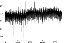
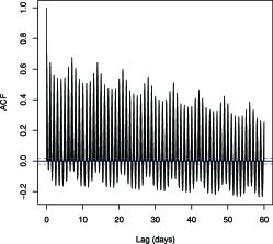
(a)	(b)
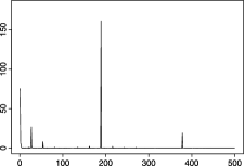
(c)

Figure 1: Time series plot, sample ACF, and periodgram of the Log transformed 30-minute (non-overlapping) aggregates. (a) Time series plot. (b) Sample ACF. (c) Periodogram.

Here, we reanalyze this dataset with the limiting aggregate seasonal long-memory model defined by (6) with $c=3$, $r=R_{1}=R_{2}=R_{3}=0$, $z_{1}=1$, $z_{2}=48$ (corresponding to daily effects), and $z_{3}=48\times 7=336$ (corresponding to weekly effects). Note that $m=30\times 60=1800$. Our new approach may be justified as the 30-minute aggregation may well fall within the intermediate asymptotic framework studied in Section 3. As discussed in Remark 3 of Section 3, we assume $D_{1}=0$. Specifically, if $\{Y_{t}\}$ is the observed time series, the spectral density function of $\{Y_{t}\}$ can be written as

$$f_{\xi,\sigma^{2}}(\omega) = \sigma^{2}\biggl{|}\sin\biggl{(}\frac{z_{1}\omega}{2}\biggr{)}\biggr{|}^{2}\biggl{|}\sin\biggl{(}\frac{z_{2}\omega}{2}\biggr{)}\biggr{|}^{-2D_{2}}\biggl{|}\sin\biggl{(}\frac{z_{3}\omega}{2}\biggr{)}\biggr{|}^{-2D_{3}}\biggl{|}\frac{\Theta_{1}(\exp(\mathrm{i}z_{1}\omega))}{\Phi_{1}(\exp(\mathrm{i}z_{1}\omega))}\biggr{|}^{2}$$

$${}\times\biggl{|}\frac{\Theta_{2}(\exp(\mathrm{i}z_{2}\omega))}{\Phi_{2}(\exp(\mathrm{i}z_{2}\omega))}\biggr{|}^{2}\biggl{|}\frac{\Theta_{3}(\exp(\mathrm{i}z_{3}\omega))}{\Phi_{3}(\exp(\mathrm{i}z_{3}\omega))}\biggr{|}^{2}\sum_{k=-\infty}^{\infty}|\omega+2k\uppi|^{-2d-2}.$$

We have considered models of orders $(P_{1},Q_{1},P_{2},Q_{2},P_{3},Q_{3})=(P_{1},Q_{1},0,0,0,0)$ with $0\leq P_{1}\leq 2$, and $0\leq Q_{1}\leq 2$. The model with the smallest AIC (Akaike information criterion) is $(P_{1},Q_{1},P_{2},Q_{2},P_{3},Q_{3})=(2,2,0,0,0,0)$. Goodness of fit of this model was studied in Chan and Tsai [5].

The spectral maximum likelihood estimates of the parameters and the $95\%$ bootstrap confidence intervals based on steps 1–4 of Section 6 of Chan and Tsai [5] are summarized in Table 2. The asymptotic standard deviations and the asymptotic $95\%$ confidence intervals are also included in Table 2. It is clear that the bootstrap confidence intervals of the parameters are comparable to their asymptotic counterparts. The confidence intervals of the parameters $d+D_{2}+D_{3}$, $D_{2}$ and $D_{3}$ indicate that the long-memory pattern, the daily seasonal long-memory pattern and the weekly seasonal long-memory pattern are all significant.

Table 2: Spectral maximum likelihood estimates of the parameters of the model defined by equation (6), with $(P_{1},Q_{1},P_{2},Q_{2},P_{3},Q_{3})=(2,2,0,0,0,0)$

		Bootstrap 95%	Asymptotic	Asymptotic 95%
	Estimated	confidence	standard	confidence
Parameter	value	interval	error	interval
$d$	$0.2326$	(0.1268, 0.2608)	0.0436	(0.1471, 0.3181)
$D_{2}$	$0.1274$	(0.1085, 0.1429)	0.0083	(0.1111, 0.1437)
$D_{3}$	$0.1271$	(0.1083, 0.1430)	0.0083	(0.1108, 0.1434)
$d+D_{2}+D_{3}$	$0.4871$	(0.3821, 0.5000)	0.0441	(0.4007, 0.5735)
$\phi_{1,1}$	$1.1277$	(0.8916, 1.5089)	0.1256	(0.8815, 1.3739)
$\phi_{1,2}$	$-0.2610$	($-$0.5773, $-$0.0508)	0.1009	($-$0.4588, $-$0.0632)
$\theta_{1,1}$	$-1.1788$	($-$1.4586, $-$0.9315)	0.0936	($-$1.3623, $-$0.9953)
$\theta_{1,2}$	$0.3593$	(0.1237, 0.5755)	0.0831	(0.1964, 0.5222)
$\sigma$	$0.3117$	(0.3017, 0.3194)	0.0051	(0.3017, 0.3217)

To assess the advantage of using the proposed aggregation model in terms of forecasting, as compared to a SARFIMA model, we divide the data roughly into two halves, with the first 5074 data for fitting the proposed model and the SARFIMA model. We use the second half of data for comparing their forecasting performance by computing $h$-step ahead predictors, for $h=1,\ldots,4000$, and the corresponding mean squared errors, via equations (5.2.19) and (5.2.20) of Brockwell and Davis [3], respectively. Specifically, the competing model we consider is a $\operatorname{SARFIMA}(2,d,2)\times(0,D_{1},0)_{s_{2}}\times(0,D_{2},0)_{s_{3}}$ model, where $s_{2}=48$, and $s_{3}=48\times 7=336$. The estimates of the parameters are $(\hat{d},\hat{D}_{2},\hat{D}_{3},\hat{d}+\hat{D}_{2}+\hat{D}_{3},\hat{\phi}_{1,1},\hat{\phi}_{1,2},\hat{\theta}_{1,1},\hat{\theta}_{1,2},\hat{\sigma})=(0.1996,0.1328,0.1280,0.4604,-0.038$, $0.8154,0.1099,-0.7342,0.1250)$. Note that the estimators of $\hat{d}$ and $\hat{d}+\hat{D}_{2}+\hat{D}_{3}$ from the SARFIMA model are smaller than those from the proposed model, which is similar to some finding reported in Section 5. Figure 2 displays the ratios (in %) of the cumulative first $h$ steps ahead mean absolute forecast errors of the SARFIMA model to their counterparts of the limiting aggregate model, for $h=1,2,\ldots,4000$. These ratios measure the long-term forecast efficiency of the proposed model relative to the SARFIMA model. As can be seen from the figure, the proposed model produces more accurate long-term forecast than the SARFIMA model once the forecast horizon is approximately longer than 1 day. We have also examined the rates the $h$-step ahead prediction variances approach their asymptotic value for the two models, and found that the fitted proposed model admits a slower convergence rate than the fitted SARFIMA model, which is consistent with the longer memory (at the zero frequency) estimated by the fitted proposed model than the SARFIMA model.

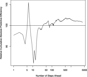
Figure 2: Long-term forecast efficiency of the proposed model relative to the SARFIMA model.

7 Concluding remarks

We have derived the limiting structure of the temporal aggregates of a (possibly non-stationary) SARFIMA model, with increasing aggregation. We have also obtained some asymptotic properties of the spectral maximum likelihood estimator of the limiting model, including consistency and asymptotic normality. Monte Carlo experiments show that the proposed method enjoys good empirical properties. Moreover, estimator of $d$ under the proposed model appears to generally have smaller bias than that from fitting a SARFIMA model to aggregate data. The efficacy of our proposed methodology is illustrated with an analysis of an internet traffic data. Model diagnostic using a bootstrap procedure in the frequency domain, as presented in Chan and Tsai [5], suggests a good fit. Future research problems include extending the model to include covariates and developing other tools for model diagnostics.

References

- [1] {bbook}[mr] \bauthor\bsnmBeran, \bfnmJan\binitsJ. (\byear1994). \btitleStatistics for Long-Memory Processes. \bseriesMonographs on Statistics and Applied Probability \bvolume61. \baddressNew York: \bpublisherChapman & Hall. \bidmr=1304490 \bptokimsref \endbibitem
- [2] {barticle}[mr] \bauthor\bsnmBisognin, \bfnmC.\binitsC. &\bauthor\bsnmLopes, \bfnmS. R. C.\binitsS.R.C. (\byear2007). \btitleEstimating and forecasting the long memory parameter in the presence of periodicity. \bjournalJ. Forecast. \bvolume26 \bpages405–427. \biddoi=10.1002/for.1030, issn=0277-6693, mr=2409792 \bptokimsref \endbibitem
- [3] {bbook}[mr] \bauthor\bsnmBrockwell, \bfnmPeter J.\binitsP.J. &\bauthor\bsnmDavis, \bfnmRichard A.\binitsR.A. (\byear1991). \btitleTime Series: Theory and Methods, \bedition2nd ed. \bseriesSpringer Series in Statistics. \baddressNew York: \bpublisherSpringer. \biddoi=10.1007/978-1-4419-0320-4, mr=1093459 \bptokimsref \endbibitem
- [4] {barticle}[mr] \bauthor\bsnmChambers, \bfnmMarcus J.\binitsM.J. (\byear1996). \btitleThe estimation of continuous parameter long-memory time series models. \bjournalEconometric Theory \bvolume12 \bpages374–390. \biddoi=10.1017/S0266466600006642, issn=0266-4666, mr=1395038 \bptokimsref \endbibitem
- [5] {bmisc}[auto:STB—2011/10/17—13:52:43] \bauthor\bsnmChan, \bfnmK. S.\binitsK.S. &\bauthor\bsnmTsai, \bfnmH.\binitsH. (\byear2008). \bhowpublishedInference of seasonal long-memory aggregate time series. Technical Report 391, Dept. Statistics & Actuarial Science, Univ. Iowa. \bptokimsref \endbibitem
- [6] {barticle}[mr] \bauthor\bsnmGranger, \bfnmC. W. J.\binitsC.W.J. &\bauthor\bsnmJoyeux, \bfnmRoselyne\binitsR. (\byear1980). \btitleAn introduction to long-memory time series models and fractional differencing. \bjournalJ. Time Ser. Anal. \bvolume1 \bpages15–29. \biddoi=10.1111/j.1467-9892.1980.tb00297.x, issn=0143-9782, mr=0605572 \bptokimsref \endbibitem
- [7] {barticle}[mr] \bauthor\bsnmHosking, \bfnmJ. R. M.\binitsJ.R.M. (\byear1981). \btitleFractional differencing. \bjournalBiometrika \bvolume68 \bpages165–176. \biddoi=10.1093/biomet/68.1.165, issn=0006-3444, mr=0614953 \bptokimsref \endbibitem
- [8] {barticle}[mr] \bauthor\bsnmHosoya, \bfnmYuzo\binitsY. (\byear1996). \btitleThe quasi-likelihood approach to statistical inference on multiple time-series with long-range dependence. \bjournalJ. Econometrics \bvolume73 \bpages217–236. \biddoi=10.1016/0304-4076(95)01738-0, issn=0304-4076, mr=1410005 \bptokimsref \endbibitem
- [9] {barticle}[mr] \bauthor\bsnmHsu, \bfnmNan-Jung\binitsN.J. &\bauthor\bsnmTsai, \bfnmHenghsiu\binitsH. (\byear2009). \btitleSemiparametric estimation for seasonal long-memory time series using generalized exponential models. \bjournalJ. Statist. Plann. Inference \bvolume139 \bpages1992–2009. \biddoi=10.1016/j.jspi.2008.09.011, issn=0378-3758, mr=2497555 \bptokimsref \endbibitem
- [10] {bincollection}[mr] \bauthor\bsnmLopes, \bfnmSílvia R. C.\binitsS.R.C. (\byear2008). \btitleLong-range dependence in mean and volatility: Models, estimation and forecasting. In \bbooktitleIn and Out of Equilibrium 2. \bseriesProgress in Probability \bvolume60 \bpages497–525. \baddressBasel: \bpublisherBirkhäuser. \biddoi=10.1007/978-3-7643-8786-0_23, mr=2477396 \bptokimsref \endbibitem
- [11] {barticle}[auto:STB—2011/10/17—13:52:43] \bauthor\bsnmMan, \bfnmK. S.\binitsK.S. &\bauthor\bsnmTiao, \bfnmG. C.\binitsG.C. (\byear2006). \btitleAggregation effect and forecasting temporal aggregates of long memory processes. \bjournalInternational Journal of Forecasting \bvolume22 \bpages267–281. \bptokimsref \endbibitem
- [12] {barticle}[auto:STB—2011/10/17—13:52:43] \bauthor\bsnmMontanari, \bfnmA.\binitsA., \bauthor\bsnmRosso, \bfnmR.\binitsR. &\bauthor\bsnmTaqqu, \bfnmM.\binitsM. (\byear2000). \btitleA seasonal fractional ARIMA model applied to Nile River monthly flows at Aswan. \bjournalWater Resources Research \bvolume36 \bpages1249–1259. \bptokimsref \endbibitem
- [13] {barticle}[mr] \bauthor\bsnmOhanissian, \bfnmArek\binitsA., \bauthor\bsnmRussell, \bfnmJeffrey R.\binitsJ.R. &\bauthor\bsnmTsay, \bfnmRuey S.\binitsR.S. (\byear2008). \btitleTrue or spurious long memory? A new test. \bjournalJ. Bus. Econom. Statist. \bvolume26 \bpages161–175. \biddoi=10.1198/073500107000000340, issn=0735-0015, mr=2420145 \bptokimsref \endbibitem
- [14] {barticle}[mr] \bauthor\bsnmPalma, \bfnmWilfredo\binitsW. &\bauthor\bsnmBondon, \bfnmPascal\binitsP. (\byear2003). \btitleOn the eigenstructure of generalized fractional processes. \bjournalStatist. Probab. Lett. \bvolume65 \bpages93–101. \biddoi=10.1016/j.spl.2003.07.008, issn=0167-7152, mr=2017253 \bptokimsref \endbibitem
- [15] {barticle}[mr] \bauthor\bsnmPalma, \bfnmWilfredo\binitsW. &\bauthor\bsnmChan, \bfnmNgai Hang\binitsN.H. (\byear2005). \btitleEfficient estimation of seasonal long-range-dependent processes. \bjournalJ. Time Ser. Anal. \bvolume26 \bpages863–892. \biddoi=10.1111/j.1467-9892.2005.00447.x, issn=0143-9782, mr=2203515 \bptokimsref \endbibitem
- [16] {barticle}[auto:STB—2011/10/17—13:52:43] \bauthor\bsnmPorter-Hudak, \bfnmS.\binitsS. (\byear1990). \btitleAn application of the seasonal fractionally differenced model to the monetary aggregates. \bjournalJ. Amer. Statist. Assoc. \bvolume85 \bpages338–344. \bptokimsref \endbibitem
- [17] {barticle}[auto:STB—2011/10/17—13:52:43] \bauthor\bsnmRay, \bfnmB. K.\binitsB.K. (\byear1993). \btitleLong-range forecasting of IBM product revenues using a seasonal fractionally differenced ARMA model. \bjournalInternational Journal of Forecasting \bvolume9 \bpages255–269. \bptokimsref \endbibitem
- [18] {barticle}[mr] \bauthor\bsnmTsai, \bfnmHenghsiu\binitsH. &\bauthor\bsnmChan, \bfnmK. S.\binitsK.S. (\byear2005). \btitleTemporal aggregation of stationary and nonstationary discrete-time processes. \bjournalJ. Time Ser. Anal. \bvolume26 \bpages613–624. \biddoi=10.1111/j.1467-9892.2005.00430.x, issn=0143-9782, mr=2188835 \bptokimsref \endbibitem
- [19] {bmisc}[auto:STB—2011/10/17—13:52:43] \bauthor\bsnmWei, \bfnmW. W. S.\binitsW.W.S. (\byear1978). \bhowpublishedSome consequences of temporal aggregation seasonal time series models. In Seasonal Analysis of Economic Time Series (A. Zellner, ed.). Washington, DC: US Department of Commerce, Bureau of Census. \bptokimsref \endbibitem