The impact of nonlocal response on metallo-dielectric multilayers and optical patch antennas

Abstract

We analyze the impact of nonlocality on the waveguide modes of metallo-dielectric multilayers and optical patch antennas, the latter formed from metal strips closely spaced above a metallic plane. We model both the nonlocal effects associated with the conduction electrons of the metal, as well as the previously overlooked response of bound electrons. We show that the fundamental mode of a metal-dielectric-metal waveguide, sometimes called the gap-plasmon, is very sensitive to nonlocality when the insulating, dielectric layers are thinner than 5 nm. We suggest that optical patch antennas, which can easily be fabricated with controlled dielectric spacer layers and can be interrogated using far-field scattering, can enable the measurement of nonlocality in metals with good accuracy.

I Introduction

With the emergence of new analytical, numerical and nanofabrication tools, the pursuit of plasmonic systems for a variety of nanophotonic applications has expanded rapidly in recent yearsmaier07 ; gramotnev2010plasmonics ; schuller2010plasmonics . Plasmonic media here can be defined as conducting surfaces and nanostructures, whose optical scattering is largely dominated by the response of the conduction electrons. Plasmonic behavior is typically associated with excitation wavelengths at which the inertial inductance of the charge carriers plays a critical role in the collective responsezhou05 . In the design of plasmonic media, the dynamics of the conduction electrons can often be well approximated by assuming a Drude-like model for the permittivity, which has the frequency dispersive form

$$\epsilon=1-\frac{\omega_{p}^{2}}{\omega^{2}+i\Gamma\omega}$$ (1)

assuming a time dependence of $e^{-i\omega\,t}$. The plasma frequency, $\omega_{p}$, proportional to the square root of the carrier density, typically lies within the ultraviolet portion of the spectrum for many metals. Thus, for frequencies just below the plasma frequency, the electric permittivity can be characterized as a lossy dielectric, for which the real part of the permittivity is moderately negative. At wavelengths where the real part of the permittivity is negative, surface plasmon modes can be supported, which are collective oscillations of the coupled electromagnetic field and conduction electrons. Surface plasmons can serve to transport energy along metal surfaces in a manner similar to dielectric waveguides, but are also playing an increasingly important role in the field of metamaterials, where metallic nanostructures are often used as elements that provide strong and customizable scattering. Surface plasmons represent the underlying mechanism behind perfect lensespendry2000negative ; fang05 , hyperlensesjacob2006optical ; liu2007far , spasersbergman03 ; zheludev08 ; oulton09 and many other proposed metamaterial-related devices.

The simplicity of the Drude model of electron response, (1), has has enabled the rapid modeling of plasmonic and metamaterial structures; The salient features associated with most plasmonic structures presented to date can usually be computed with sufficient accuracy –sometimes even analytically– assuming the Drude formula. Particularly when the underlying physics is the main focus rather than detailed performance characteristics, Eq. (1) frequently provides an adequate description of the plasmonic response. It should be noted that despite the relatively simple form of Eq. (1), the numerical simulation of plasmonic systems remains a non-trivial task because the surface plasmon spatial variation is not limited by the wavelength of light; rather, the surface plasmon can confine light to nanometer sized regions, making plasmonic structures an inherently multiscale modeling problemkottmann00 . Thus, the frequency dispersion and the negative permittivity associated with the Drude model contain non-trivial physics, and have been successfully applied to a wide range of plasmonic and metamaterial configurations. Naturally, the actual electronic response of a metal or highly doped semiconductor is much more complicated than that suggested by Eq. (1). Plasmonic structures are now reliably fabricated at the nanometer and sub-nanometer scales, where new optical properties arise that cannot be accounted for solely by the Drude modelscholl12 ; fernandez12 . Since these sub-nanometer features are likely to be crucial for optimizing field localization and enhancementpendry12 ; ciraci12 ; moreau12 , a more detailed description of the properties of plasmonic devices is demanded. Effects that would be secondary or of no consequence to the overall function of prior plasmonic devices, may introduce major constraints on the detailed performance and ultimate competitiveness of optimized plasmonic structures with subnanometer features. For these reasons, it is relevant to consider a more advanced physical model of the carrier response in conductors.

The Drude model of a conductor assumes only the participation of conduction electrons (no bound charges), and further assumes a straightforward force-response relationship between the applied electric field and responding current density. An intrinsic feature of this model is that the responding current density at a given point within the material is proportional to the electric field at that point; that is, the Drude model assumes locality. Even when the exact, measured values of the bulk permittivity are used, there is an implicit assumption of locality since the permittivity is only a function of frequency rather than of both frequency and wave vector. To capture the additional physics associated with electronic response, it is necessary to consider a more detailed model of the force-response relationship between the field and current density.

More accurate descriptions of the free electron gas have been proposed in the past, including a description based on a hydrodynamical model for the conduction electronskliewer68 ; barrera81 ; boardman82 ; gerhardts84 ; forstmann86 ; fuchs87 ; fuchs1981dynamical ; scalora10 , and a microscopic description initiated by Feibelmanfeibelman82 ; liebsch1997electronic ; wang11 . The latter has been improved over the yearsliebsch1995influence and has been recently used to include the effects of nonlocality on metallic slabsruppin05b and slot waveguideswang07 . The hydrodynamical approach clearly suffers from an uncertainty about which additional boundary conditions should be used, but allows for more transparent physical interpretationsfuchs1981dynamical . Moreover, the hydrodynamical model can be reasonably implemented in numerical calculations, and also is useful for finding closed-form, analytical results. For example, the hydrodynamical model has been used in conjunction with transformation optics techniques to find analytical expressions for nanostructures that illustrate the impact of nonlocal responsependry12 ; fernandez12 . Recent experiments have shown that the hydrodynamical model is able to describe very accurately the plasmon resonance shift exhibited by spherical nanoparticles interacting with a metallic filmciraci12 . While the hydrodynamical model is clearly not the most sophisticated approach to describe the free electron gas, it can obviously capture the physics of nonlocality and it seems it can be made quite accurate through a correct choice of the free parameters it contains for situations of interest in plasmonics.

In the present work, we first try to describe the response of the bound electrons as a polarizable medium, as has been shown to be accurate for Feibelman’s methodliebsch1995influence , but in the framework of the hydrodynamical model. We find that this description greatly simplifies the discussion with respect to the additional boundary conditions. We explore the consequences of the model on the reflection of a wave by a metallic surface, on the surface plasmon and finally on the propagation of a guided wave along a thin metallic waveguide, as Wang and Kempa have shown that nonlocal effects could be expectedwang07 for such a structure. Using an analytical dispersion relation, we show that the nonlocal effects are enhanced in the slow light regime, when the waveguide is a few nanometers thick. Finally we study the large impact of nonlocality on optical patch nanoantennasmiyazaki2006controlled ; bozhevolnyi07 ; sondergaard08 ; jung09 ; yang12 where the gap beneath the patch behaves as a cavity, making these structures extremely sensitivemoreau12 . The optical patch geometry paves the way for future experiments in which the effects associated with nonlocality will have easily measurable effects at wavelengths in the visible.

II Nonlocal response of metals

While our analysis is not specific to metals, we use the term metal throughout while keeping in mind the analysis can be applied to highly doped semiconductorshoffman07 and potentially other conducting systemstassin12 . The polarization of a metal, and hence its dielectric function, generally contains contributions from both bound and free conduction electrons. Because we need to apply different physical response models to the free and bound electrons, it is essential to first distinguish their relative contributions. The experimental permittivity curves can be fitrakic98 with a Drude term (1) that models the free electron contribution, to which is added a sum over the Brendel-Bormannbrendel1992infrared oscillator terms that models the susceptibility arising from the bound electron contributions. Figure 1 shows the permittivity of gold obtained through the model as well as the fitted Drude permittivity, corresponding to $1+\chi_{f}$, where $\chi_{f}$ is the the susceptibility of the free electrons. The difference (not shown) between the modeled permittivity and the fitted Drude term corresponds to the contribution of the bound electrons, $\chi_{b}$.

We assume here that the nonlocal response of the metal is largely dominated by the nonlocality induced by free electrons, so that we can treat the bound electron contribution as purely local, as some authors domcmahon09 ; mcmahon10 ; fernandez12 . Bound electrons too can be expected to present a nonlocal response, similar to what occurs in dielectricsmaradudin73 ; agranovich . Our assumption is equivalent to assuming that the interactions between electrons in a free electron gas (through a quantum pressure and Coulomb repulsion) are more intense than essentially dipole-dipole interaction between bound electrons.

Figure 1: Real part of the relative permittivity of gold in the visible (solid line) and Drude permittivity according to rakic98 (dotted line). The difference is the contribution of bound electrons. Inset : imaginary part of the relative permittivity, same $x$ scale, same lines.

Under an applied electric field, the medium will undergo a polarization with contributions from both bound and free electrons. The total polarization vector can thus be written

$$\mathbf{P}=\mathbf{P}_{b}+\mathbf{P}_{f}$$ (2)

where $\mathbf{P}_{b}=\epsilon_{0}\chi_{b}\mathbf{E}$, $\chi_{b}$ being the susceptibility of the bound electrons, with the currents in the free electron gas related to the polarization in the usual manner:

$$\dot{\mathbf{P}}_{f}=\mathbf{J}.$$ (3)

By incorporating all responding currents and charges into the polarization, we can treat the metal as a dielectric, such that the electric flux density, $\mathbf{D}=\epsilon_{0}\mathbf{E}+\mathbf{P}_{b}+\mathbf{P}_{f}$, satisfies $\mathbf{\nabla}\cdot\mathbf{D}=0$. Taking the divergence of $\mathbf{D}$ and writing $\mathbf{P}_{b}$ in terms of the electric field, we obtain

$$\mathbf{\nabla}\cdot\mathbf{P}_{f}=-\epsilon_{0}(1+\chi_{b})\,\mathbf{\nabla}\cdot\mathbf{E}.$$ (4)

where we have explicitly assumed that the bound electron susceptibility is local and can be taken outside the divergence operator.

The free electron current density can be related to the applied electric field using the hydrodynamical model. Using Eq. 2, a linearized equation relating $\mathbf{P}_{f}$ to the electric field is given byscalora10

$$-\beta^{2}\,\mathbf{\nabla}\left(\mathbf{\nabla}\cdot\mathbf{P}_{f}\right)+\ddot{\mathbf{P}}_{f}+\gamma\dot{\mathbf{P}}_{f}=\epsilon_{0}\omega_{p}^{2}\mathbf{E}$$ (5)

where $\gamma$ is the damping factor, due to collisions of the electron gas with the ion grid, $\omega_{p}$ is the plasma frequency of the metal, and $\beta$ is the phenomenological nonlocal parameter, proportional to the Fermi velocity $v_{F}$. Usually the value of $\beta=\sqrt{\frac{2}{3}}v_{F}$ has been considered in the literature. However, a slightly more realistic hydrodynamic model should take into account other sources of nonlocality, such as the Bohm potential, which can be shown to be of the same order of the Fermi pressurecrouseilles08 . Though it is beyond the scope of this paper to introduce a more sophisticated model, it makes sense from a phenomenological approach to consider a more empirical value for the parameter $\beta$. Recently it has been shown for plasmonic systems of film-coupled gold nanoparticles that the value $\beta=\sqrt{\frac{5}{3}\frac{E_{F}}{m}}\simeq 1.27\times 10^{6}~{}\rm{m/s}$ gives a very good agreement with experimental dataciraci12 . In this work we will then assume this former value for both gold and silver.

Assuming a harmonic solution of the form $e^{-i\omega t}$, and using equation 4, the polarization $\mathbf{P}_{f}$ can finally be written

$$\mathbf{P}_{f}=-\epsilon_{0}\frac{\omega_{p}^{2}}{\omega^{2}+i\gamma\omega}\left(\mathbf{E}-(1+\chi_{b})\,\frac{\beta^{2}}{\omega_{p}^{2}}\,\mathbf{\nabla}\left(\mathbf{\nabla}\cdot\mathbf{E}\right)\right),$$ (6)

where the term

$$\chi_{f}=-\frac{\omega_{p}^{2}}{\omega^{2}+i\gamma\omega}$$ (7)

can be identified as the local susceptibility associated with free electrons, corresponding to the Drude model.

We have written the polarization terms in such a manner that the free and bound electron contributions can be distinguished. In determining the various parameters in these equations for the calculations that follow, we use the model provided byrakic98 and shown Fig. 1.

III Transverse and longitudinal modes in metals

In a metal, taking the above description of nonlocality into account, Maxwell’s equations can now be written

$$\mathbf{\nabla}\times\mathbf{E} =i\omega\mu_{0}\mathbf{H}$$ (8)

$$\mathbf{\nabla}\times\mathbf{H} =-i\omega\left(\epsilon_{0}(1+\chi_{b})\mathbf{E}+\mathbf{P}_{f}\right)$$ (9)

$$=-i\omega\epsilon_{0}\epsilon\left(\mathbf{E}-\alpha\mathbf{\nabla}\left(\mathbf{\nabla}\cdot\mathbf{E}\right)\right)$$ (10)

where $\epsilon$ is the local relative permittivity of the metal

$$\epsilon=1+\chi_{b}+\chi_{f}$$ (11)

and

$$\alpha =\frac{\chi_{f}\,(1+\chi_{b})}{\epsilon}\,\frac{\beta^{2}}{\omega_{p}^{2}}$$ (12)

$$=\frac{\beta^{2}}{\frac{\omega_{p}^{2}}{1+\chi_{b}}-\omega^{2}-i\gamma\omega}.$$ (13)

As shown rigorously in the appendix, there are two different solutions to these equations corresponding to two different kinds of waves. The first solution satisfies $\mathbf{\nabla}\cdot\mathbf{E}=0$, so that it corresponds to the standard solution to Maxwell’s equations when the nonlocality is overlooked. Equations (8) and (10) become

$$\mathbf{\nabla}\times\mathbf{E} =i\omega\mu_{0}\mathbf{H}$$ (14)

$$\mathbf{\nabla}\times\mathbf{H} =-i\omega\epsilon_{0}\epsilon\mathbf{E},$$ (15)

Finally all the fields satisfy Helmholtz’s equation

$$\nabla^{2}\mathbf{H}+\epsilon\,k_{0}^{2}\mathbf{H}=\mathbf{0},$$ (16)

where $k_{0}=\frac{\omega^{2}}{c^{2}}$. Since the divergence of the electric field is zero, the electric field is orthogonal to the wavevector when the wave is propagative, which means it is transverse. The dispersion relation for these transverse waves is thus

$$\mathbf{k}^{2}=\epsilon\,k_{0}^{2}=\epsilon\,\frac{\omega^{2}}{c^{2}}.$$ (17)

The second kind of solution is curl free, which means it satisfies $\mathbf{\nabla}\times\mathbf{E}=\mathbf{0}$ and there is no accompanying magnetic field. These waves are called longitudinal because when they are propagative, the electric field is parallel to the wavevector. They correspond to bulk plasmons: oscillations of the free electron gas due to the pressure term. Since the divergence of the electric field is not identically zero, there exists a charge density inside the metal given by

$$\rho=\epsilon_{0}\mathbf{\nabla}\cdot\mathbf{E}.$$ (18)

Equation (10), then yields the wave equation for the bulk plasmons

$$\mathbf{\nabla}\left(\mathbf{\nabla}\cdot\mathbf{E}\right)-\frac{1}{\alpha}\mathbf{E}=\nabla^{2}\mathbf{E}-\frac{1}{\alpha}\mathbf{E}=\mathbf{0}.$$ (19)

and the corresponding dispersion relation is

$$\mathbf{k}^{2}=-\frac{1}{\alpha}=\frac{1}{\beta^{2}}\left(\omega^{2}-\frac{\omega_{p}^{2}}{1+\chi_{b}}+i\gamma\omega\right).$$ (20)

An alternative way to write this dispersion relation is

$$\epsilon_{\parallel}\equiv 1+\chi_{b}-\frac{\omega_{p}^{2}}{\omega^{2}+i\gamma\omega-\beta^{2}\mathbf{k}^{2}}=0,$$ (21)

which is the way previous works have taken $\chi_{b}$ into accountfernandez12 through a so-called longitudinal permittivity. But the equation governing the polarization $\mathbf{P}_{f}$ (equation (5)) cannot be deduced from the longitudinal permittivity using a simple Fourier transformmcmahon09 ; mcmahon10 , as has been previously pointed outraza11 .

Figure 2: Dispersion relation for transverse waves (thick lines) and bulk plasmons (thin lines) when (a) the nonlocality is absent ($\beta=0$) and (b) the nonlocality is important. The dashed lines show the imaginary parts of the propagation constants for the transverse and longitudinal waves, below the plasma frequency $\omega_{p}$. When nonlocality is present, for a given $\omega$ two waves must be taken into account.(color online)

The dispersion relations, Eqs. (17) and (20), are plotted in Fig. 2 for two cases of the nonlocal parameter $\beta$, for the simplified case where $\epsilon=1-\frac{\omega_{p}^{2}}{\omega^{2}}$. For small $\beta$, the longitudinal mode disperses very little, and can be generally ignored in wave propagation problems. When $\beta$ is nonzero, however, the longitudinal mode acquires dispersion, and is generally present at a given frequency of excitation. Above the plasma frequency, both the transverse and longitudinal modes are propagating, while below the plasma frequency both modes decay exponentially. In considering boundary value problems, it is clear that a wave incident on a half space filled with a nonlocal, plasmonic medium will generally couple to both types of waves. To avoid the system being underdetermined, an additional boundary condition must be used as will be discussed in the subsequent section.

Figure 3: A simple interface between a dielectric and a metal.

Let us now consider a multilayered structure, that could be as simple as the single interface shown in figure 3, invariant in two directions, here taken as $x$ and $y$. The $z$ axis is thus perpendicular to any interface considered, as shown in Fig. 3. Without any loss of generality, it is possible to assume solutions that are translationally invariant along the $y$ (out-of-plane) direction. As shown in the appendix, the system of equations (8) and (10) can be split into two subsystems corresponding to $s$ (electric field polarized perpendicular to the plane of incidence) and $p$ (magnetic field polarized perpendicular to the plane of incidence) polarizations. Moreover, we will assume from now on that all the fields present an $x$ dependence that varies as $e^{ik_{x}\,x}$ (or, equivalently, we take the Fourier transform along the $x$ axis).

For the $s$ polarization, $\mathbf{\nabla}\times\mathbf{E}=\mathbf{0}$ yields $E_{y}=0$, so that no bulk plasmon can be excited. Nonlocality has then no impact on this polarization, so that we will deal in the following with $p$ polarization only.

Equation (16) then yields

$$\partial_{z}^{2}H_{y}=-(\epsilon\,k_{0}^{2}-k_{x}^{2})\,H_{y},$$ (22)

so that the magnetic field can be written

$$H_{y}=(A\,e^{i{k_{z}}_{t}\,z}+B\,e^{-i{k_{z}}_{t}\,z})\,e^{ik_{x}\,x-i\omega\,t}$$ (23)

with ${k_{z}}_{t}=\sqrt{\epsilon\,k_{0}^{2}-k_{x}^{2}}$ where $k_{0}=\frac{\omega}{c}$. The $E_{x}$ and $E_{z}$ accompanying fields can be found using equations

$$E_{x} =\frac{1}{i\omega\epsilon_{0}\,\epsilon}\partial_{z}H_{y}$$ (24)

$$E_{z} =-\frac{1}{i\omega\epsilon_{0}\,\epsilon}\partial_{x}H_{y}.$$ (25)

For longitudinal waves, the wave equation (19) becomes

$$\partial_{z}^{2}E_{x}=\left(k_{x}^{2}+\frac{1}{\alpha}\right)\,E_{x}\,.$$ (26)

For normal incidence (for $k_{x}=0$), depending whether $\omega$ is smaller or larger than $\frac{\omega_{p}}{\sqrt{1+\chi_{b}}}$, the bulk plasmon will be respectively evanescent ($\Re(\alpha)>0$) or propagative ($\Re(\alpha)<0$) . In the visible range, we usually have $\omega<\frac{\omega_{p}}{\sqrt{1+\chi_{b}}}$ so that the bulk plasmon is evanescent and the above equation can be solved to yield

$$E_{x}=(C\,e^{\kappa_{l}\,z}+D\,e^{-\kappa_{l}\,z})\,e^{ik_{x}\,x-i\omega\,t}$$ (27)

with

$$\kappa_{l}^{2} =\frac{1}{\beta^{2}}\left(\frac{\omega_{p}^{2}}{1+\chi_{b}}-\omega^{2}-i\gamma\omega\right)+k_{x}^{2}$$ (28)

$$=k_{x}^{2}+\frac{\omega_{p}^{2}}{\beta^{2}}\left(\frac{1}{\chi_{f}}+\frac{1}{1+\chi_{b}}\right).$$ (29)

The fact that longitudinal waves are curl-free yields

$$E_{z}=\frac{1}{ik_{x}}\partial_{z}E_{x},$$ (30)

which allows determination of the contribution of the bulk plasmon to $E_{z}$ if needed.

IV Additional boundary conditions

The nonlocal nature of the metal results in the appearance of a longitudinal bulk plasmon mode that can be excited from the metal interface, in addition to the surface-localized plasmon polariton. The well-known Maxwell’s boundary conditions are not sufficient to uniquely define the amplitudes of these independent waves. More specifically, for each metallic layer, two new unknowns are introduced and must be resolved in the solution of the electromagnetic boundary value problem. To avoid dealing with an underdetermined problem then, additional boundary conditions must be imposed at the metal interface.

The issue of boundary conditions has been abundantly discussed in the context of spatially dispersive crystals, and a variety of different boundary conditions has been proposedagranovich ; halevi84 . In the context of the hydrodynamic model, the choice of boundary conditions is much simplerboardman82 ; forstmann86 , essentially because fewer types of waves are involved. Two additional boundary conditions are typically considered in the case of an interface between a metal and a dielectric, when the contribution of the bound electrons is overlooked: either (i) $P_{z}=0$boardman82 ; forstmann86 or (ii) the continuity of $E_{z}$ruppin05 ; fernandez12 . If the considered dielectric is vacuum, then these two conditions are equivalent. Condition (i) can be justified because the polarization in the metal is due to actual currents; since the electrons are not allowed to leave the metal, then the normal current must vanish at the interface and also the polarization. Condition (ii) can be justified by treating the interface as smooth for all fields, including the normal component of the electric field.

In our description of the response of metals, the susceptibility attributed to bound electrons, $\chi_{b}$ is considered purely local. One might expect that the equation $\mathbf{\nabla}\cdot\mathbf{D}=0$ would impose a supplementary condition (namely the continuity of $D_{z}$), leaving no freedom in the choice of the boundary condition. This is however not the case: in multilayered systems, the continuity of $H_{y}$ through an interface implies the continuity of $D_{z}$, so that an additional boundary condition is still required.

The response of the metal in our description is partly the response of a standard dielectric medium, so that there is no reason to assume the continuity of $E_{z}$ at the surface of the metal. Condition (ii) thus appears very difficult to support when the contribution of bound electrons is taken into account as a local, polarizable medium.

The underlying physicsboardman82 ; forstmann86 behind condition (i), that free electrons cannot escape the metal, does however not lead here to $P_{z}=0$ at the edge of the metal because not all the polarization comes from actual currents in the free electron gas. It is thus not reasonable to use boundary condition (i) for the case when bound electrons contribute to the polarization response.

It would be physically reasonable to consider that only the polarization linked to actual current leaving the metal should be zero at the interface between a metal and a dielectric. For multilayered structures, this condition can be written

$${P_{f}}_{z}=0.$$ (31)

at the interface as an additional boundary condition. We underscore that this boundary condition is not equivalent to conditions (i) and (ii) when the outside medium is vacuum.

In the case of an interface between two metals, again, condition (i) is hard to justify, but the interface obviously should not be considered as impervious to free electrons. Instead, it would sound to consider that the currents, and thus the polarization $\mathbf{P}_{f}$, should be continuous. This would actually provide the two additional boundary conditions that are required for an interface between two metals. Although we will not consider here structures involving such an interface, we emphasize that taking into account the contribution of bound electrons to the response of metals seem to lead to unambiguous boundary conditions based on physical reasoning.

V Reflection from a metallic surface

Let us now consider an incident plane wave coming from above ($z>0$) and propagating in a dielectric medium with a permittivity $\epsilon_{d}$, reflected by a metallic interface located at $z=0$, as shown in Fig. 3 - the metal being characterized by a permittivity $\epsilon$.

For $p$ polarization, the magnetic field in the dielectric region can be then written

$$H_{y}=\left(e^{-ik_{z}\,z}+r\,e^{ik_{z}\,z}\right)\,e^{ik_{x}\,x-i\omega\,t}$$ (32)

where $k_{z}=\sqrt{\epsilon_{d}\,k_{0}^{2}-k_{x}^{2}}$ and $k_{0}=\frac{\omega}{c}$, while the electric field along the $x$ direction has the form

$$E_{x}=\frac{ik_{z}}{i\omega\epsilon_{0}\epsilon_{d}}\,\left(r\,e^{ik_{z}\,z}-e^{-ik_{z}\,z}\right)\,e^{ik_{x}\,x-i\omega\,t}.$$ (33)

In the metal, the magnetic field can be written

$$H_{y}=A\,e^{\kappa_{t}\,z}\,e^{ik_{x}\,x-i\omega\,t}$$ (34)

where $\kappa_{t}=\sqrt{k_{x}^{2}-\epsilon\,k_{0}^{2}}$, and the electric field

$$E_{x} =\left(\frac{\kappa_{t}}{i\omega\epsilon_{0}\epsilon}A\,e^{\kappa_{t}\,z}+B\,e^{\kappa_{l}\,z}\right)\,e^{ik_{x}\,x-i\omega\,t}$$ (35)

$$E_{z} =\left(-\frac{ik_{x}}{i\omega\epsilon_{0}\epsilon}A\,e^{\kappa_{t}\,z}+\frac{\kappa_{l}}{ik_{x}}\,B\,e^{\kappa_{l}\,z}\right)\,e^{ik_{x}\,x-i\omega\,t}.$$ (36)

The magnetic field $H_{y}$ and the $x$ component of the electric field $E_{x}$ are continuous at $z=0$ so that

$$1+r =A$$ (37)

$$(r-1)\frac{ik_{z}}{\epsilon_{d}} =\frac{\kappa_{t}}{\epsilon}\,A+i\omega\epsilon_{0}\,B.$$ (38)

Since ${P_{f}}_{z}=-\frac{1}{i\omega}\,\partial_{x}H_{y}-\epsilon_{0}(1+\chi_{b})\,E_{z}$, the condition ${P_{f}}_{z}=0$ in the metal at the interface, can be written

$$ik_{x}\,A\,\left(\frac{1}{\epsilon}-\frac{1}{1+\chi_{b}}\right)=\frac{\kappa_{l}}{ik_{x}}\,i\omega\epsilon_{0}\,B$$ (39)

Finally $A$ and $B$ can be eliminated to yield

$$r=\frac{\frac{ik_{z}}{\epsilon_{d}}+\frac{\kappa_{t}}{\epsilon}-\Omega}{\frac{ik_{z}}{\epsilon_{d}}-\frac{\kappa_{t}}{\epsilon}+\Omega}$$ (40)

where

$$\Omega=\frac{k_{x}^{2}}{\kappa_{l}}\left(\frac{1}{\epsilon}-\frac{1}{1+\chi_{b}}\right)$$ (41)

The reflection coefficient indicates that the bulk plasmon is not excited at normal incidence for $k_{x}=0$ because in that case only one component of the electric field is present in the incident and reflected fields. When the angle of incidence increases the excitation of the bulk plasmon is more and more important because of the increasing $E_{z}$ component. Of course $\kappa_{l}$ is increasing too, which means that the bulk plasmon penetration is more shallow, but only slightly - so that the $\Omega$ increases essentially as $k_{x}^{2}$.

VI Surface plasmon

If the field is not propagative in the dielectric region, but has the form

$$H_{y}=\left(C\,e^{\kappa_{z}\,z}+D\,e^{-\kappa_{z}\,z}\right)\,e^{ik_{x}\,x-i\omega\,t}$$ (42)

with $\kappa_{z}=\sqrt{k_{x}^{2}-\epsilon_{d}\,k_{0}^{2}}=-ik_{z}$, then it is meaningless to define a reflection coefficient (40), but still we can write that

$$\frac{D}{C}=\frac{\frac{\kappa_{z}}{\epsilon_{d}}-\frac{\kappa_{t}}{\epsilon}+\Omega}{\frac{\kappa_{z}}{\epsilon_{d}}+\frac{\kappa_{t}}{\epsilon}-\Omega}$$ (43)

The surface plasmon is a solution for which $D\neq 0$ and $C=0$, thus corresponding to a pole of the left hand side of equation (43), and a zero of its denominator, so that the dispersion relation can be written

$$\frac{\kappa_{z}}{\epsilon_{d}}+\frac{\kappa_{t}}{\epsilon}=\Omega$$ (44)

The larger the propagation constant $k_{x}$, the larger $\Omega$ and thus the larger the impact of nonlocality. However, for surface plasmons, very large values of $k_{x}$ are difficult to reach (typically, the maximum effective index is around 1.4 for a silver-air interface) as shown in figure 4. The impact of nonlocality on bare surface plasmons is thus very small. In the following, we will see that for a metal-dielectric-metal waveguide with a very thin dielectric layer, the impact of nonlocality on the guided mode is much more important because very large $k_{x}$ values can be reached whatever the wavelength.

Figure 4: Dispersion relation ($\omega$ as a function of $k_{x}$) for a surface plasmon at the interface between silver and air. The local description (thick solid curve) can almost not be distinguished from the nonlocal description (thick dashed curve, almost identical with the thick solid curve). In order to illustrate the effect of nonlocality, we show here (dotted line) the impact of an exaggerated nonlocality ($\beta$ multiplied by ten). The thin solid curve is $\omega=k_{x}\,c$.

VII The impact of boundary conditions

The form of the reflection coefficient and to the dispersion relation above clearly show that $\Omega$ is the parameter controlling the influence of the nonlocality on propagation phenomena. Moreover, it makes manifest the consequences of a change in the boundary conditions.

In the literature, the entire metal response is often attributed to the free electrons, while the response of bound electrons is neglectedboardman82 ; forstmann86 ; ruppin05 . When the bound electron response is neglected, the dispersion relation of the bulk plasmon yields

$$\kappa_{l}=\sqrt{k_{x}^{2}+\frac{\omega_{p}^{2}}{\beta^{2}}\left(\frac{1}{\chi_{f}}+1\right)}$$ (45)

instead of

$$\kappa_{l}=\sqrt{k_{x}^{2}+\frac{\omega_{p}^{2}}{\beta^{2}}\left(\frac{1}{\chi_{f}}+\frac{1}{1+\chi_{b}}\right)}$$ (46)

where a local contribution from bound electrons is assumedfernandez12 .

If the boundary condition with the dielectric is chosen to be the continuity of the component of the electric field normal to the interface, then we have

$$\Omega=\frac{k_{x}^{2}}{\kappa_{l}}\left(\frac{1}{\epsilon}-\frac{1}{\epsilon_{d}}\right),$$ (47)

where $\kappa_{l}$ can be calculated using one of the above expressions, depending on the description of the metal’s properties. When the entire polarization $P_{z}$ is chosen to vanish at the interface, we have instead

$$\Omega=\frac{k_{x}^{2}}{\kappa_{l}}\left(\frac{1}{\epsilon}-1\right).$$ (48)

In the following, we will investigate all the different descriptions that are presented in table 1 to show that, even if they differ regarding the quantitative impact of nonlocality, they all at least agree qualitatively.

Descr.	$\kappa_{l}^{2}$	A.B.C.	$\Omega$
1	$k_{x}^{2}+\frac{\omega_{p}^{2}}{\beta^{2}}\left(\frac{1}{\chi_{f}}+1\right)$	$P_{z}(0)=0$	$\frac{k_{x}^{2}}{\kappa_{l}}\left(\frac{1}{\epsilon}-1\right)$
2	$k_{x}^{2}+\frac{\omega_{p}^{2}}{\beta^{2}}\left(\frac{1}{\chi_{f}}+1\right)$	$E_{z}$ continuous	$\frac{k_{x}^{2}}{\kappa_{l}}\left(\frac{1}{\epsilon}-\frac{1}{\epsilon_{d}}\right)$
3	$k_{x}^{2}+\frac{\omega_{p}^{2}}{\beta^{2}}\left(\frac{1}{\chi_{f}}+\frac{1}{1+\chi_{b}}\right)$	$P_{z}=0$	$\frac{k_{x}^{2}}{\kappa_{l}}\left(\frac{1}{\epsilon}-1\right)$
4	$k_{x}^{2}+\frac{\omega_{p}^{2}}{\beta^{2}}\left(\frac{1}{\chi_{f}}+\frac{1}{1+\chi_{b}}\right)$	$E_{z}$ continuous	$\frac{k_{x}^{2}}{\kappa_{l}}\left(\frac{1}{\epsilon}-\frac{1}{\epsilon_{d}}\right)$
5	$k_{x}^{2}+\frac{\omega_{p}^{2}}{\beta^{2}}\left(\frac{1}{\chi_{f}}+\frac{1}{1+\chi_{b}}\right)$	${P_{f}}_{z}=0$	$\frac{k_{x}^{2}}{\kappa_{l}}\left(\frac{1}{\epsilon}-\frac{1}{1+\chi_{b}}\right)$

Table 1: Summary of the different descriptions of nonlocality. The first two do not consider separately the contribution from the bound electrons, the last three do. The last one is the one that is preferred in this work.

VIII Metal-dielectric-metal waveguide

While the impact of nonlocality can be considered minor for the single interface problem above, nonlocal effects can be far more evident in multilayer systems. In metallo-dielectric layers, it is possible to reduce the thickness of layers to the nanometer or even sub-nanometer scale; modes that propagate in such layers can be significantly confined, to the point where local models are forced to break down. For this reason, multilayer systems and structures based on multilayers can be useful as an experimental tool to investigate and measure nonlocal effects.

In this section, we consider the case of a dieletric with a permittivity $\epsilon_{d}$ sandwiched between two metallic surfaces (as shown in figure 5) and study more thoroughly the influence of the nonlocality of the metal on the first even guided mode (the fundamental mode).

Figure 5: Metallic waveguide of width $h$.

VIII.1 Dispersion relation

We consider here a symmetric waveguide, the metal being the same on both sides of the dielectric layer. The magnetic field in the dielectric can be written as

$$H_{y}=\left(C\,e^{\kappa_{z}\,z}+D\,e^{-\kappa_{z}\,z}\right)\,e^{ik_{x}\,x-i\omega\,t}\,.$$ (49)

As we have seen in the previous section, at $z=-\frac{h}{2}$, we have

$$\frac{D\,e^{\kappa_{z}\,\frac{h}{2}}}{C\,e^{-\kappa_{z}\,\frac{h}{2}}}=\frac{\frac{\kappa_{z}}{\epsilon_{d}}-\frac{\kappa_{t}}{\epsilon}+\Omega}{\frac{\kappa_{z}}{\epsilon_{d}}+\frac{\kappa_{t}}{\epsilon}-\Omega}$$ (50)

while for $z=+\frac{h}{2}$ (the $z$ axis has to be reversed, which means $C$ and $D$ should be exchanged)

$$\frac{C\,e^{\kappa_{z}\,\frac{h}{2}}}{D\,e^{-\kappa_{z}\,\frac{h}{2}}}=\frac{\frac{\kappa_{z}}{\epsilon_{d}}-\frac{\kappa_{t}}{\epsilon}+\Omega}{\frac{\kappa_{z}}{\epsilon_{d}}+\frac{\kappa_{t}}{\epsilon}-\Omega}.$$ (51)

Combining these two equations, we get

$$e^{2\kappa_{z}\,h}=\left(\frac{\frac{\kappa_{z}}{\epsilon_{d}}-\frac{\kappa_{t}}{\epsilon}+\Omega}{\frac{\kappa_{z}}{\epsilon_{d}}+\frac{\kappa_{t}}{\epsilon}-\Omega}\right)^{2}=r^{2}$$ (52)

and finally either the mode is symetrical ($C=D$) and we have $r=e^{\kappa_{z}\,h}$ which can be written

$$\frac{\kappa_{z}}{\epsilon_{d}}\tanh\frac{\kappa_{z}\,h}{2}+\frac{\kappa_{t}}{\epsilon}=\Omega$$ (53)

or the mode is antisymetrical ($C=-D$), which means $r=-e^{\kappa_{z}\,h}$ and finally

$$\frac{\kappa_{z}}{\epsilon_{d}}\coth\frac{\kappa_{z}\,h}{2}+\frac{\kappa_{t}}{\epsilon}=\Omega.$$ (54)

VIII.2 Nature of the guided modes

We first discuss the nature of the guided modes in a thin metallic waveguide. There are two situations that are clear and for which the guided modes of the structure have well-posed definitionsmaier07 :

• The perfect metallic waveguide, which supports a fundamental mode that is flat and that has no cut-off (it is supported whatever the thickness of the metallic waveguide). In addition, we have analytical expressions for the propagation constant and field profile of all the modes. For the fundamental mode, we have

  $$k_{x}^{2}=\epsilon_{d}\,k_{0}^{2}$$ (55)

• The plasmonic (i.e. wide) metallic waveguide, which supports coupled surface plasmonsmaier07 . At a given frequency and for a wide enough guide, the even and the odd surface plasmon modes present propagation constants that can be arbitrarily close to the propagation constant of the surface plasmon

  $$k_{x}=k_{0}\,\sqrt{\frac{\epsilon_{d}\,\epsilon(\omega)}{\epsilon_{d}+\epsilon(\omega)}},$$ (56)

  even for complex values of $\epsilon(\omega)$.

For the case of a thin (a few nanometers) waveguide we seek the best description to retain for the only guided mode found.

Consider the case of coupled surface plasmons first. We can approach the condition of a perfect metallic waveguide by making the permittivity of the metal change such that its real part tends towards infinity. As can be seen in figure6 the odd mode tends towards the fundamental mode but the field inside the dielectric (index of 1.58) always stays evanescent. The even mode tends towards the first even mode of the perfect metallic waveguide and the field becomes propagative at some point (where the real part of the propagation constant becomes smaller than the optical index of the dielectric). The point at which the field of the even mode becomes propagative could even be defined as a limit between the “coupled surface plasmon” and the “perfect metallic waveguide” pictures.

Figure 6: Trajectory in the complex plane of the quantity $\frac{k_{x}}{k_{0}}$ for three different waveguided modes (solid line: first even mode; dashed line: first odd mode ; dotted line: second even mode) when the permittivity of the metal goes from $\epsilon=-10+i$ (circles) to $\epsilon=-2000+i$, for a thickness of the waveguide of 500 nm and a dielectric with an 1.58 optical index. The intermediate value of $-100+i$ is indicated on the curves.

Now consider starting with a large waveguide (500 nm) and decreasing its width down to a few nanometers. As can be seen in figure 7, the even mode presents an increasing propagation constant. The odd mode, by contrast, presents a decreasing propagation constant - the field in the dielectric even becomes propagative as in the previous case. For thin layers (smaller than 128 nm here) this mode presents a very large imaginary part and a very small real part: it can be considered as evanescent in the $x$ direction even if the cut-off cannot be defined precisely.

Figure 7: Trajectory in the complex plane of the quantity $\frac{k_{x}}{k_{0}}$ for three different waveguided modes (solide line: first even mode; dashed line: first odd mode ; dotted line: second even mode) when the width of the metal goes from 380 nm (circles) to 10 nm. The permittivity of the metal is taken equal to the permittivity of gold at 608 nm, $\epsilon\simeq-10.01+1.44i$. Intermediate thickness of $221$ nm (when the real part of the index of the odd mode becomes smaller than 1.58, so that the coupled plasmon picture becomes less relevant), $128$ nm (when the odd mode can be considered non-propagative, and the coupled plasmon picture is not relevant any more) and $50$ nm are indicated on the curves. .

For a small dielectric thickness, the waveguide thus behaves much more like a perfect metallic waveguide (a fundamental mode with no cut-off, no propagative even mode) and except for the fact that the field of the first even mode is evanescent in the $z$ direction, has not much to do with the coupled surface plasmons situation. This is why we refer to this mode as the fundamental mode of the waveguide.

This mode is however sometimes called gap-plasmon in the literaturejung09 , a term that underscores the differences between the actual mode and the fundamental more of a perfect metallic waveguide.

VIII.3 Nonlocal effects

When the waveguide becomes extremely thin, as can be seen in figure 7, the effective index (and thus $k_{x}$) of the fundamental mode (with a dispersion relation given by (53)) can become arbitrary large. When $k_{x}$ is larger, $\Omega$ is larger, which means that the non-locality has a much larger impact on the mode’s propagation constant. It is possible to compare (see figures 8, 9 for a waveguide filled with a dielectric with a 1.58 optical index) the local effective index as a function of the waveguide’s width with a local and with a nonlocal theory. Obviously the impact of nonlocality is limited for $h>5$ nm but it can become very important under that threshold. The parameters we have considered for gold are given in rakic98 and $\beta=1.27.10^{6}$ m/sscalora10 ; ciraci12 .

Figure 8: Effective index of the guided mode at 600 nm, as a function of the dielectric width, $h$. The dispersion relations are shown for different descriptions (see table 1): the completely local case (thin black curve, top), $P_{z}(0)=0$ (description 1, dash-dotted line) and $E_{z}$ continuous (description 2, dashed line) with no identified contribution of the bound electrons, and descriptions separating the contributions of bound and free electrons, with $P_{z}=0$ (description 3, dash-double dotted line), a continuous $E_{z}$ (description 4, thin dash line) and finally our description (description 5, thick solid curve), that is preferred in this work.

Figure 9: Same as figure 8 except for the log scale.

Since different descriptions of nonlocality exist in the literature, we have compared our approach to the other descriptions available (different boundary conditions, as well as considering that the whole response of the medium is nonlocal or not, as described in section VII and summarize in table 1).

The hydrodynamic model is often said to exaggerate nonlocal effects. It could be expected that taking into account the response of the bound electrons, which can be considered as local, would lower the impact of nonlocality on the guided mode compared to when the whole response of the metal is considered nonlocal. Figures 8 and 9 show that this is paradoxically not the case when the boundary condition that we consider as being the most physical (${P_{f}}_{z}=0$) is not chosen. Considering a separate response of the bound electrons actually lowers the effective plasma frequency, as explained above, which leads to a deeper penetration of the field corresponding to the bulk plasmons, which may in turn increase the importance of this field (depending, of course, on the boundary conditions).

When the condition we propose is used, the impact of nonlocality is even lower than when considering a completely nonlocal response of the metal and using $P_{z}=0$. This actually makes us think the boundary condition we propose here, is not only the most sound physically, but it may even yield an more accurate estimate of the nonlocal effects.

IX Cavity resonances for metallic strips coupled to a metallic film

Many structures and phenomena rely on the fundamental mode of the metallic waveguide like the enhanced transmission by subwavelength slit arrayscao02 ; moreau07 ; collin07 , highly absorbent gratingsleperchec08 or strip nanoantennasbozhevolnyi07 ; sondergaard08 ; jung09 ; yang12 to mention a few. The latter are patches that are invariant perpendicularly to the plane (see Fig. 10). The mode that is guided between a strip and the metallic film, whose dispersion relation is given by (53) as long as the patch is thick enough, if reflected by the edges of the strip. The reflection coefficient $r$ of the mode can be computed easilymoreau07 using a Fourier Modal Methodlalanne96 ; granet96 . When the strip is wide enough, Fabry-Perot resonances may occurjung09 .

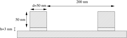
Figure 10: Strips (rods with a 50 nm by 50 nm section) are separated from the metallic film by a 3 nm thick dielectric with an optical index of 1.58. The structure considered here is periodic, with a 200 nm period.

The local energy density (and hence the absorption) should be proportional to the square of the field amplitude, given by a Fabry-Perot formulamoreau07 , yielding

$$\left|\mathbf{H}\right|^{2}=\left|\frac{1}{1-r^{2}\,e^{2i\,k_{x}\,d}}\right|^{2}.$$ (57)

This model allows the accurate prediction of the position of the resonance when a purely local response of the metal is assumed, as shown figure 11: the resonance predicted using model (57) ($k_{x}$ being computed using dispersion relation Eq. (53) with $\Omega=0$) occurs exactly where there is a dip in the reflectance of the nanorods covered surface. This confirms the physical analysis of the structure and that a one-mode model is sufficient to describe the resonances.

As we have shown above, when nonlocality is taken into account, the propagation constant $k_{x}$ of the guided mode differs from the purely local case. That is why the resonances of the nanorods can be expected to be very sensitive to nonlocality when the thickness of the spacer is typically smaller than 5 nm.

Full COMSOL simulations based on the hydrodynamical model with the boundary conditions we suggest in this work (description 5 in table 1) show that the resonance of the structure is largely blueshifted compared to the purely local simulations. This is completely accounted for by model (57) when using a propagation constant $k_{x}$ computed using the dispersion relation (53) and keeping the same coefficient reflection $r$ as for the local case. This proves that nonlocality intervenes almost only through the change of the propagation constant of the guided mode, and not at all through a change of the reflection coefficient.

Figure 11: Bottom : Reflection spectrum according to local (RCWA, dashed line) and nonlocal (COMSOL, solid line) simulations. Top : Model (57) for the field intensity under the strips for the local (dashed line) and nonlocal (solid line) theory. The agreement between the simulations and the model are in excellent agreement for the local as well as for the nonlocal theory.

Such structures, or structures presenting a very similar behaviourmoreau12 , are obviously a way to assess experimentally the effects of nonlocality on the guided mode of the metallic waveguide with a good accuracy.

X Conclusion

We have proposed in this work an improvement of the hydrodynamic model by clearly separating the nonlocal response of the free electrons, and the response of the bound electrons, considered as localliebsch1995influence . Such a distinction makes the discussion about the additional boundary conditions much more clear, leaving nothing but a single condition that seems physically sound: no current of free electrons leaving the metal. We have shown that this condition leads to a lower impact of the nonlocality than many other descriptions based on the hydrodynamic model. This description may thus answer two main concerns regarding this kind of models compared to Feibelman’s approachfeibelman82 ; wang11 : the uncertainty about the boundary conditions and a tendency to exagerate the effects of nonlocality. Furthermore, recent experimental results have shown that the hydrodynamical model can describe nonlocal effects very accuratelyciraci12 . Given the reduced complexity of the hydrodynamic model relative to full quantum and other microscopic models of electron response, it is of continued interest to further explore the accuracy of these models in the context of plasmonic nanostructures.

Following previous work on slot waveguides that support gap plasmonswang07 , we have shown that the slow light regime reached when the waveguide is only a few nanometers thick is responsible for a large enhancement of the nonlocal effects. Using these results, we have studied the impact of nonlocality on patch nanoantennas and shown that it should be easy to detect, paving the way for future experiments.

Our analysis is of relevance to numerous nanophotonic devices, including metallodielectric waveguides, nanoantennas and nanocavities, which rely on the excitation of gap plasmons on very thin, conducting layers for their operationmiyazaki2006controlled ; bozhevolnyi07 ; sondergaard08 ; jung09 ; yang12 . These resonant structures have a variety of diverse applications, for instance, as highly efficient concentrators and absorbers of lightleperchec08 ; moreau12 . The description of conductors we provide can also prove useful when testing the limits of the classical theory for describing structures containing metals or doped semiconductors, for which the response of the bound electrons are strong.

As has been once more shown here, the hydrodynamic model yields analytical results that help to understand the underlying physics of nonlocalityfuchs1981dynamical ; ruppin05 . It presents the supplementary avantage of being easy to use in simulations with complex geometriesciraci12 . The analytical calculations we have presented, beyond the clarification they may bringmcmahon09 ; mcmahon10 , are thus a first step towards the extension of widely used numerical methodsgranet96 ; lalanne96 ; krayzel10 to account accurately for nonlocality.

Appendix I

Let us write equations (8) and (10) within the metal in Cartesian coordinates in the case where the fields do not depend on $y$ :

$$-\partial_{z}E_{y} =i\omega\,\mu_{0}\,H_{x}$$ (58)

$$\partial_{z}E_{x}-\partial_{x}E_{z} =i\omega\,\mu_{0}\,H_{y}$$ (59)

$$\partial_{x}E_{y} =i\omega\,\mu_{0}\,H_{z}$$ (60)

$$-\partial_{z}H_{y} =-i\omega\epsilon_{0}\epsilon\left(E_{x}-\alpha\partial_{x}^{2}E_{x}-\alpha\partial_{x}\partial_{z}E_{z}\right)$$ (61)

$$\partial_{z}H_{x}-\partial_{x}H_{z} =-i\omega\epsilon_{0}\epsilon E_{y}$$ (62)

$$\partial_{x}H_{y} =-i\omega\epsilon_{0}\epsilon\left(E_{x}-\alpha\partial_{z}^{2}E_{z}-\alpha\partial_{x}\partial_{z}E_{x}\right)$$ (63)

This system of equations can be split into two subsystems corresponding to $s$ (electric field polarized perpendicular to the plane of incidence) and $p$ (magnetic field polarized perpendicular to the plane of incidence) polarizations. The $s$ subsystem is identical to the subsystem without taking nonlocality into account, because of the simple form of equation (62). Nonlocality has then no impact on this polarization, so that we will deal in the following with $p$ polarization only.

The subsystem concerning the $p$ polarization can be written

$$\partial_{z}E_{x}-\partial_{x}E_{z} =i\omega\,\mu_{0}\,H_{y}$$ (64)

$$-\alpha\partial^{2}_{x}E_{x}+E_{x}-\alpha\partial_{x}\partial_{z}E_{z} =\frac{1}{i\omega\epsilon_{0}\,\epsilon}\partial_{z}H_{y}$$ (65)

$$-\alpha\partial^{2}_{z}E_{z}+E_{z}-\alpha\partial_{x}\partial_{z}E_{x} =-\frac{1}{i\omega\epsilon_{0}\,\epsilon}\partial_{x}H_{y}$$ (66)

By applying the operator $-\alpha\partial_{x}\partial_{z}$ to equation (66), operator $1-\alpha\partial^{2}_{z}$ to equation (65) and subtracting one resulting equation from the other, one gets

$$\left(1-\alpha\left(\partial^{2}_{x}+\partial^{2}_{z}\right)\right)E_{x}=\frac{\left(1-\alpha\left(\partial^{2}_{x}+\partial^{2}_{z}\right)\right)}{i\omega\epsilon_{0}\,\epsilon}\partial_{z}H_{y}.$$ (67)

Repeating the same procedure, but applying $1-\alpha\partial^{2}_{x}$ to equation (66), $-\alpha\partial_{x}\partial_{z}$ to equation (65), and subtracting the resulting equation from the other we obtain the decoupled system of equations

$$\partial_{z}E_{x}-\partial_{x}E_{z} =i\omega\,\mu_{0}\,H_{y}$$ (68)

$$\left(1-\alpha\left(\partial^{2}_{x}+\partial^{2}_{z}\right)\right)E_{x} =\frac{\left(1-\alpha\left(\partial^{2}_{x}+\partial^{2}_{z}\right)\right)}{i\omega\epsilon_{0}\,\epsilon}\partial_{z}H_{y}$$ (69)

$$\left(1-\alpha\left(\partial^{2}_{x}+\partial^{2}_{z}\right)\right)E_{z} =-\frac{\left(1-\alpha\left(\partial^{2}_{x}+\partial^{2}_{z}\right)\right)}{i\omega\epsilon_{0}\,\epsilon}\partial_{x}H_{y}.$$ (70)

We can apply the inverse of the differential operator $1-\alpha\left(\partial^{2}_{x}+\partial^{2}_{z}\right)$ to both sides of the equations to obtain the classical system

$$\partial_{z}E_{x}-\partial_{x}E_{z} =i\omega\,\mu_{0}\,H_{y}$$ (71)

$$E_{x} =\frac{1}{i\omega\epsilon_{0}\,\epsilon}\partial_{z}H_{y}$$ (72)

$$E_{z} =-\frac{1}{i\omega\epsilon_{0}\,\epsilon}\partial_{x}H_{y}.$$ (73)

This system is identical with that corresponding to a purely local response of the metal and its solution satisfies $\mathbf{\nabla}\cdot\mathbf{E}=0$. The wave that it describes is referred to as the transverse wave because when it is propagative, the electric field is orthogonal to the propagation vector.

But to this solution should be added any solution for which

$$-\alpha\left(\partial^{2}_{x}+\partial^{2}_{z}\right)E_{x}+E_{x} =0$$ (74)

$$-\alpha\left(\partial^{2}_{x}+\partial^{2}_{z}\right)E_{z}+E_{z} =0$$ (75)

$$-\alpha\left(\partial^{2}_{x}+\partial^{2}_{z}\right)H_{y}+H_{y} =0.$$ (76)

because it would also be a solution of system 68. Using (74) along with (65) and (64), it is not difficult to show that $H_{y}=0$ so that this solution satisfies

$$\partial_{z}E_{x}=\partial_{x}E_{z}.$$ (77)

References

- (1) S. A. Maier, Plasmonics: fundamentals and applications (Springer Verlag, 2007)
- (2) D. K. Gramotnev and S. I. Bozhevolnyi, Nature Photonics 4, 83 (2010)
- (3) J. A. Schuller, E. S. Barnard, W. Cai, Y. C. Jun, J. S. White, and M. L. Brongersma, Nature materials 9, 193 (2010)
- (4) J. Zhou, T. Koschny, M. Kafesaki, E. N. Economou, J. B. Pendry, and C. M. Soukoulis, Physical review letters 95, 223902 (2005)
- (5) J. B. Pendry, Physical Review Letters 85, 3966 (2000)
- (6) N. Fang, H. Lee, C. Sun, and X. Zhang, Science 308, 534 (2005)
- (7) Z. Jacob, L. V. Alekseyev, and E. Narimanov, Optics Express 14, 8247 (2006)
- (8) Z. Liu, H. Lee, Y. Xiong, C. Sun, and X. Zhang, Science 315, 1686 (2007)
- (9) D. J. Bergman and M. I. Stockman, Physical review letters 90, 27402 (2003)
- (10) N. Zheludev, S. Prosvirnin, N. Papasimakis, and V. Fedotov, Nature Photonics 2, 351 (2008)
- (11) R. Oulton, V. Sorger, T. Zentgraf, R. Ma, C. Gladden, L. Dai, G. Bartal, and X. Zhang, Nature 461, 629 (2009)
- (12) J. P. Kottmann, O. J. F. Martin, D. R. Smith, and S. Schultz, Opt. Express 6, 213 (2000)
- (13) J. A. Scholl, A. L. Koh, and J. A. Dionne, Nature 483, 421 (2012)
- (14) A. I. Fernandez-Dominguez, A. Wiener, F. J. Garcia-Vidal, S. A. Maier, and J. B. Pendry, Physical Review Letters 108, 106802 (2012)
- (15) J. Pendry, A. Aubry, D. Smith, and S. Maier, science 337, 549 (2012)
- (16) C. Ciracì, R. Hill, J. Mock, Y. Urzhumov, A. Fernández-Domínguez, S. Maier, J. Pendry, A. Chilkoti, and D. Smith, Science 337, 1072 (2012)
- (17) A. Moreau, C. Ciracì, R. T. Hill, J. J. Mock, Q. Wang, B. J. Wiley, A. Chilkoti, and D. R. Smith, Nature 492, 86 (2012)
- (18) K. Kliewer and R. Fuchs, Physical Review 172, 607 (1968)
- (19) R. G. Barrera and A. Bagchi, Physical Review B 24, 1612 (1981)
- (20) A. D. Boardman, Electromagnetic surface modes (Wiley, 1982)
- (21) R. R. Gerhardts and K. Kempa, Physical Review B 30, 5704 (1984)
- (22) F. Frostmann and R. R. Gerhardts, Metal optics near the plasma frequency, Vol. 109 (Springer-Verlag, 1986)
- (23) R. Fuchs and F. Claro, Physical Review B 35, 3722 (1987)
- (24) R. Fuchs and R. G. Barrera, Physical Review B 24, 2940 (1981)
- (25) M. Scalora, M. A. Vincenti, D. de Ceglia, V. Roppo, M. Centini, N. Akozbek, and M. J. Bloemer, Phys. Rev. A 82, 043828 (2010)
- (26) P. Feibelman, Progress in Surface Science 12, 287 (1982)
- (27) A. Liebsch, Electronic excitations at metal surfaces (Springer, 1997)
- (28) Y. Wang, E. Plummer, and K. Kempa, Advances in Physics 60, 799 (2011)
- (29) A. Liebsch and W. L. Schaich, Physical Review B 52, 14219 (1995)
- (30) R. Ruppin and K. Kempa, Physical Review B 72, 153105 (2005)
- (31) X. Wang and K. Kempa, Physical Review B 75, 245426 (2007)
- (32) H. T. Miyazaki and Y. Kurokawa, Applied physics letters 89, 211126 (2006)
- (33) S. I. Bozhevolnyi and T. Søndergaard, Optics Express 15, 10869 (2007)
- (34) T. Søndergaard, J. Beermann, A. Boltasseva, and S. I. Bozhevolnyi, Physical Review B 77, 115420 (2008)
- (35) J. Jung, T. Søndergaard, and S. I. Bozhevolnyi, Physical Review B 79, 035401 (2009)
- (36) J. Yang, C. Sauvan, A. Jouanin, S. Collin, J. Pelouard, and P. Lalanne, Optics Express 20, 16880 (2012)
- (37) A. J. Hoffman, L. Alekseyev, S. S. Howard, K. J. Franz, D. Wasserman, V. A. Podolskiy, E. E. Narimanov, D. L. Sivco, and C. Gmachl, Nature Materials 6, 946 (2007)
- (38) P. Tassin, T. Koschny, M. Kafesaki, and C. M. Soukoulis, Nature Photonics(2012)
- (39) A. D. Rakic, A. B. Djurišic, J. M. Elazar, and M. L. Majewski, Applied Optics 37, 5271 (1998)
- (40) R. Brendel and D. Bormann, Journal of applied physics 71, 1 (1992)
- (41) J. M. McMahon, S. K. Gray, and G. C. Schatz, Physical review letters 103, 097403 (2009)
- (42) J. M. McMahon, S. K. Gray, and G. C. Schatz, Physical Review B 82, 035423 (2010)
- (43) A. A. Maradudin and D. L. Mills, Physical Review B 7, 2787 (1973)
- (44) V. M. Agranovich and V. L. Ginzburg, Crystal optics with spatial dispersion, and excitons (Springer-Verlag Berlin, 1984)
- (45) N. Crouseilles, P. A. Hervieux, and G. Manfredi, Phys. Rev. B 78, 155412 (2008)
- (46) S. Raza, G. Toscano, A. P. Jauho, M. Wubs, and N. A. Mortensen, Physical Review B 84, 121412 (2011)
- (47) P. Halevi and R. Fuchs, Journal of Physics C: Solid State Physics 17, 3869 (1984)
- (48) R. Ruppin, Journal of Physics: Condensed Matter 17, 1803 (2005)
- (49) Q. Cao and P. Lalanne, Phys. Rev. Lett. 88, 057403 (2002)
- (50) A. Moreau, C. Lafarge, N. Laurent, K. Edee, and G. Granet, J. Opt. A : Pure Appl. Opt. 9, 165 (2007)
- (51) S. Collin, F. Pardo, and J. L. Pelouard, Opt. Express 15, 4310 (2007)
- (52) J. LePerchec, P. Quemerais, A. Barbara, and T. Lopez-Rios, Phys. Rev. Lett. 100, 066408 (2008)
- (53) P. Lalanne and G. M. Morris, J. Opt. Soc. Am. A 13, 779 (1996)
- (54) G. Granet and B. Guizal, J. Opt. Soc. Am. A 13, 1019 (1996)
- (55) F. Krayzel, R. Pollès, A. Moreau, M. Mihailovic, and G. Granet, J. Europ. Opt. Soc. Rap. Pub. 5, 10025 (2010)