Three different approaches to the same interaction: the Yukawa model in nuclear physics

Abstract

After a brief discussion of the meaning of the potential in quantum mechanics, we shall examine the results of the Yukawa model (scalar meson exchange) for the nucleon-nucleon interaction in three different dynamical frameworks: the non-relativistic dynamics of the Schrodinger equation, the relativistic quantum mechanics of the Bethe-Salpeter and Light-Front equations and the lattice solution of the Quantum Field Theory, obtained in the quenched approximation.

1 Introduction

Since Newton’s time, an interaction between two particles is understood as something that prevents their relative motion to be rectilinear and uniform. In non-relativistic Quantum Mechanics this is realized by any operator $\hat{V}$, traditionally called potential, that disturbs a plane wave $|k\rangle$, i.e. there is no any constant $\lambda$ such that

$$(H_{0}+\hat{V})\mid k\rangle={\lambda}\mid k\rangle$$

while

$$H_{0}\mid k\rangle=E\mid k\rangle$$

$E$ being the energy of the state $|k\rangle$.

From where does the potential $\hat{V}$ come from? Sometimes it is taken from classical mechanics, like in the Coulomb case, but it can be picked out of a hat as well, provided one respects some space-time (translation, rotation, P, T) or internal (C, isospin) symmetries.

This way to built an interaction is perfectly legal and can be even extended in order to satisfy the requirements of relativistic invariance. The proper method of constructing the Poincare algebra with a given $\hat{V}$ was formulated in the series of works by Bakamjiam and Thomas [1], extended later by Keister and Polyzou [2].

From this point of view, particles interact because they go into an inhomogeneous region of the space: if $\hat{V}$ was a constant, nothing would happen. This “ex nihilo” approach, though leading to some remarkable success, has not been very fertile when describing the physical phenomena, specially in the subatomic world. Here is the crucible where deep changes in the states of matter occur, one of the deepest being the non-conservation of the particle number, like in the annihilation of matter into light, $e^{+}+e^{-}\to\gamma+\gamma$, or, conversely, the transform of “speed” into matter-antimatter pairs like in $p+p\to p+p+\bar{p}+p$, both processes which are nowadays customary in the laboratories. The potential approach of the non-relativistic quantum mechanics with a fixed number of particles is here of a little help. Even worst, it does not provide any “way of thinking” about the natural processes.

A more interesting approach is provided by the Quantum Field Theory (QFT), now customary in the high energy physics world. In QFT, the interaction is a consequence of the exchange of a bosonic mediator field. This approach has been successfully applied since the development of quantum electrodynamics to every piece of the Standard Model of particle physics. In the Lagrangian formulation, the simplest case is provided by the Yukawa model [3]. The interaction between fermionic matter fields $\Psi$ is mediated by a scalar field $\Phi$ and written in terms of the Lagrangian as:

$${\cal L}(x)={\cal L}_{D}[\Psi]+{\cal L}_{KG}[\Phi]+{\cal L}_{int}[\Psi,\Phi]$$

where:

$${\cal L}_{int}(x)=g\bar{\Psi}(x)\;\Phi(x)\;\Psi(x)$$

and ${\cal L}_{D}$, ${\cal L}_{KG}$ are respectivley the Dirac and Klein-Gordon free Lagrangians.

Within this framework, a particle on a free state $|k_{1}\rangle$ emits a quanta $|q\rangle$ which is absorbed by a particle on a state $|k_{2}\rangle$. Their initial states are modified in the process and results into new ones $|k^{\prime}_{1}\rangle$ and $|k^{\prime}_{2}\rangle$ : they have “interacted”.

Figure 1: Lowest order exchange graph.

$$k_{1} \to k^{\prime}_{1}=k_{1}-q$$ (1)

$$k_{2} \to k^{\prime}_{2}=k_{1}+q$$ (2)

The basic element of this “lego” is the annihilation-creation-creation in the interaction vertex, driven by a strength constant $g_{0}$:

$$g\;a^{\dagger}_{k^{\prime}_{1}}\;b^{\dagger}_{q}\;a_{k^{\phantom{{}^{\prime}}}_{1}}\quad\rightarrow\quad g\;a^{\dagger}_{k^{\prime}_{1}}e^{-ik^{\prime}_{1}x_{1}}\;b^{\dagger}_{q}e^{iqx_{1}}\;a_{k_{1}}e^{ik_{1}x_{1}}\quad\rightarrow\quad g\;\bar{\Psi}(x_{1})\Phi(x_{1})\Psi(x_{1})$$

and Quantum Field Theory tells us how to associate to the process displayed in Fig. 1 a probability amplitude $A(k_{1},k_{2}\to k^{\prime}_{1},k^{\prime}_{2})$.

The relation between the QFT and the potential approach is made by identifying $V$ to the amplitude of the lowest order “exchange” graph, which according to Feynman rules reads

$$V\equiv\frac{1}{4m^{2}}A(k_{1},k_{2}\to k^{\prime}_{1},k^{\prime}_{2})=\frac{1}{4m^{2}}\bar{u}(k_{1})u(k^{\prime}_{1})\;{g^{2}\over q^{2}-\mu^{2}}\;\bar{u}(k_{2})u(k^{\prime}_{2})\ .$$ (3)

The potential $V(\vec{r})$ used in non-relativistic quantum mechanics is obtained by a Fourier transform of the amplitude $A$ after some – quite crude – simplifications:

$$\bar{u}(k_{1})u(k^{\prime}_{1}) = \bar{u}(k_{2})u(k^{\prime}_{2})=2m$$

$$q = (0,\vec{q})=(0,\vec{k}_{1}-\vec{k}_{2})$$

One thus obtains

$$V(k_{1},k_{2},k^{\prime}_{1},k^{\prime}_{2})=V(q)={-}{g^{2}\over\mu^{2}+\vec{q}^{2}}$$

and, by a three-dimensional Fourier transform, the usual Yukawa potential

$$V(r)=-{g^{2}\over 4\pi}\;{e^{-\mu r}\over r}$$ (4)

is obtained. This is the procedure leading to the usual $1/r$ Coulomb potential starting from QED. The same that brought Yukawa to formulate the first theory of strong interactions that deserved him a Noble prize.

Some remarks are in order:

(i) If the interaction was limited to only one exchange of Fig. 1, there would never exist a bound state. These states are indeed associated to poles in the scattering amplitude, and the Born term (one exchange term) has no one. An infinite sum of exchanges is needed to generate these singularities and this task is ensured by the dynamical equations

$$(H_{0}+V)|\Psi\rangle=E|\Psi\rangle\quad\Longrightarrow\quad T=V+VG_{0}T=V+VG_{0}V+VG_{0}VG_{0}V+\ldots$$ (5)

Series (5) generates a pole in the scattering amplitude according to the well known recipe: $1+x+x^{2}+\ldots={1\over 1-x}$, named “ladder sum”.

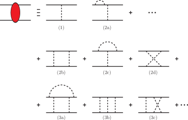
Figure 2: Perturbative expansion of the scattering amplitude.

(ii) The ladder sum, used in all nuclear models, accounts only for a small, though infinite, part of the full interaction given by ${\cal L}_{int}$. At any order in the coupling constant, there are several contributions which are ignored. Figure 2 illustrates the perturbative series of the scattering amplitude: diagrams (2a), (2c) and (2d) are of the same order than (2b) but are not included in Eq. (5). It is even worse at higher orders, since the fraction of dropped diagrams increases very fast.

Even assuming that the effect of some of the neglected diagrams is incorporated in the renomalized quantities – e.g. (2a) in the mass and (2c) in the coupling constant – there remains an infinity of them. If $g$ is large, what one neglects is not negligible and one can expect that the physics with $\hat{V}$ could seriously depart from the ones contained in the underlying ${\cal L}_{\rm int}$.

We present in what follows the results obtained when the very same interaction – the Yukawa model – is considered in three different dynamical approaches. They will be limited to the $J^{\pi}=0^{+}$ bound states and corresponding low energy scattering parameters.

Apart from being at the origin of the theory of nuclear forces, this model, the simplest meson-fermion interaction Lagrangian, has several advantages: (i) in the non-relativistic limit it gives the same result for the two-fermion and the two-boson system, (ii) when inserted in the relativistic equations – at least the ones considered here – it does not require any regularization procedure to be integrated and (iii) it is a renormalizable quantum field theory.

Section 2 is devoted to the non-relativistic results. They are widely used and constitute the reference ground of most of the nuclear and atomic physics calculations. In section 3 we will consider the results of two relevant, relativistic equations: the Bethe-Salpeter [4, 5] and Light-Front Dynamics [6]. Section 4 will contain the quantum field results obtained using the lattice techniques in the quenched approximation.

2 Non-relativistic results

We consider in this section the non-relativistic system of two particles with equal mass $m$, interacting by a Yukawa potential (4) of strength $g$ and range parameter $\mu$.

Although the problem depends on three parameters ($m,g,\mu$) it can be shown that the binding energy ($B$) and the scattering length ($a_{0}$) are given by

$$B = m\;\left(\frac{\mu}{m}\right)^{2}\varepsilon(G)$$ (6)

$$a_{0} = {1\over\mu}\;\lambda(G)$$ (7)

where $\varepsilon(G)$ and $\lambda(G)$ are respectively the binding energy and scattering length of the dimensionless S-wave Schrodinger equation:

$$u^{\prime\prime}(x)+\left[-\varepsilon+G\;{e^{-x}\over x}\right]u(x)=0$$ (8)

with a coupling constant $G$, related to the original parameters ($m,g,\mu$) by

$$G={g^{2}\over 4\pi}\;{m\over\mu}$$

Figure 3: Ground state binding energy of the dimensionless non-relativistic Yukawa model (8) as a function of the coupling constant $G$. The appearance of the first bound state corresponds to $G_{0}=1.680$.

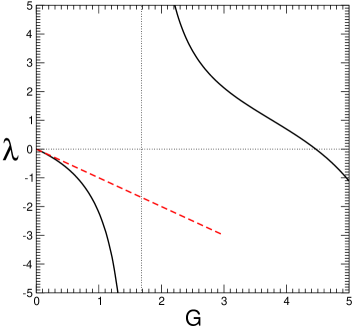
Figure 4: Scattering length in the same model than Fig. 4. The Born approximation is indicated by the dashed line. The singularity (vertical line) corresponds to the appearance of the first bound state.

The functions $\varepsilon(G)$ and $\lambda(G)$ are displayed in Figs. 4 and 4 respectively. The convention used for the scattering length corresponds to $\delta(k)=-a_{0}k+o(k^{2})$. The critical value for the appearance of the ground state is $G_{0}\approx 1.680$. At this value $\lambda(G)$ has a pole and it can be shown that for small values of G one has

$$\lambda(G)=-G+o(G^{2})$$ (9)

which corresponds to the Born approximation. All the physics of the non-relativistic problem (S-wave) is contained in these two figures, with the understanding that there exists an infinity of similar branches in $B(G)$ – and corresponding poles in $\lambda(G)$ – at increasing values of G ($G_{0}=1.680,G_{1}=6.445,G_{2}=14.34,\ldots$) indicating the appearance of an infinite number of excited states.

In summary, for a massive exchange $\mu$, there is a non-zero minimal value of the coupling constant $g_{0}$ required to have the first bound state. It is given by ${g_{0}}^{2}(m,\mu)=4\pi G_{0}{\mu\over m}$ with $G_{0}\approx 1.680$. This $g_{0}$ value decreases linearly with $\mu$ and vanishes in the Coulomb limit ($\mu\to 0$) but in the nuclear case ($\mu/m\approx 0.5$) is rather large $g_{0}\approx 3$. Once the bound state appears, the solutions of Eq. (8) exist for any value of the parameter $G$ and one can obtain any value for the binding energy $B$, even exceeding $2m$,

3 The Yukawa model in Relativistic Dynamics

Things become less simple when considering the same model in a relativistic framework. This covers a very wide and –to some extent– not well defined domain of theoretical physics aiming to incorporate all or part of the relativistic invariance in the dynamical equations. It goes from the simple implementation of relativistic kinematics to the full Quantum Field Theory treatment, which will be the proper way to incorporate relativity to the quantum world but whose solutions are very difficult to obtain beyond the perturbative domain.

We will consider here two of the many relativistic approaches: the Light Front Dynamics (LFD) and the Bethe-Salpeter (BS) equation. Although far from being representative of this vast domain they illustrate well the kind of qualitative agreements and quantitative differences in the predictions they give. Both are rooted in the Quantum Field Theory but present important differences in the way they are constructed as well as in the formal objects they deal with.

The BS equation deals with a field theoretical object corresponding to the following amplitude [5]:

$$\Phi(x_{1},x_{2},P)=\langle 0|T\left\{\Psi(x_{1})\bar{\Psi}(x_{2})\right\}|P\rangle$$ (10)

where $P^{2}=M^{2}$ is the total mass of the two-body system.

It is usually written in momentum space $\Phi(k,P)$, obtained after taking into account translational invariance and performing a Fourier transform with respect to the relative coordinate $x=x_{1}-x_{2}$:

$$\Phi(x_{1},x_{2},P)=\frac{1}{(2\pi)^{3/2}}\;\tilde{\Phi}(x,P)\;e^{-iP\makebox[2.27626pt]{$\cdot$}(x_{1}+x_{2})/2}$$

$$\tilde{\Phi}(x,P)=\int\frac{d^{4}x}{(2\pi)^{4}}\;\Phi(k,P)\;e^{-ik\makebox[2.27626pt]{$\cdot$}x}.$$

The BS amplitude for a two-fermions system is a $4\times 4$ matrix in spinor space which can be expanded in a basis of independent Dirac structures $S^{(c)}$

$$\Phi=\sum_{c=1}^{n_{c}}\phi_{c}\;S^{(c)}\qquad S^{(c)}\in\left\{1,\gamma_{\mu},\gamma_{5},\gamma_{\mu}\gamma_{5},\sigma_{\mu\nu}\right\}$$ (11)

The number of scalar components $n_{c}$ depends on the quantum number of the state. For $J=0^{+}$ there are four of them which can be chosen as:

$$\Phi(k,P)=\phi_{1}(k,P)\gamma_{5}+\phi_{2}(k,P){\hat{P}\over M}\gamma_{5}+\phi_{3}(k,P)\left[{(k\makebox[2.27626pt]{$\cdot$}P)\hat{P}\over M^{3}}-{\hat{k}\over M}\right]\gamma_{5}+\phi_{4}(k,P){i\sigma_{\mu\nu}P_{\mu}k_{\nu}\over M^{2}}$$ (12)

where $\hat{k}=\gamma^{\mu}k_{\mu}$ and $\sigma_{\mu\nu}={i\over 2}[\gamma_{\mu},\gamma_{\nu}]$.

The dynamical equation can be represented in the following graphical form:

For the case of two equal mass fermions it reads

$$S_{1}^{-1}(k_{1})\Phi(k,P)\bar{S}_{2}^{-1}(k_{2})=\int\frac{d^{4}k^{\prime}}{(2\pi)^{4}}\;iK(k,k^{\prime})\;\Gamma_{1}\;\Phi(k^{\prime},P)\;\bar{\Gamma}_{2}$$ (13)

where

$$S_{1}(k_{1}) = \frac{i}{\hat{k}_{1}-m+i\epsilon}\;\;\;,\qquad\qquad k_{1}={P\over 2}+k$$

$$\bar{S}_{2}(k_{2}) = \frac{i}{-\hat{k}_{2}-m+i\epsilon}\;,\qquad\qquad k_{2}={P\over 2}-k$$

are the fermion propagators. $\Gamma_{i}$ and $K$ are respectively the vertex functions and the meson propagator. They depend on the particular type of meson-fermion coupling. In the case of the Yukawa model (scalar meson exchange) they are

$$K(k,k^{\prime},p)=\frac{1}{(k-k^{\prime})^{2}-\mu^{2}+i\epsilon}.$$ (14)

and

$$\Gamma_{1}=\Gamma_{2}=\bar{\Gamma}_{2}=-ig$$

The BS equation (13) in momentum space is four dimensional. After a partial wave expansion it reduces to a set of coupled two-dimensional equations among the different components $\phi_{c}$ of the state (11). This equation has been solved by several authors for the bound state problem both in the Euclidean [7, 8] and Minkoswki metric [9, 10] and for the on-mass shell scattering amplitudes [11, 12, 13]. For the scattering states, the full (off-shell) solution in Minkowski space has been obtained only very recently [14, 15, 16].

LFD can be understood as an Hamiltonian formulation of the QFT defined on an space-time surface of equation $\omega\makebox[2.27626pt]{$\cdot$}x=\sigma$, where $\omega$ is a light cone vector $\omega^{2}=0$ [6].

The state vector $|\Psi(\sigma)\rangle$ is defined on this plane and the Poincaré algebra generators are obtained by integrating through this surface the flux of the conserved Noether currents associated to a given Lagrangian ${\cal L}$. In case of translations, for instance, they are given by

$$\hat{P}^{\mu}(\sigma)=\int T^{\mu\nu}(x)\delta(\omega\makebox[2.27626pt]{$\cdot$}x-\sigma)\;\omega_{\nu}d^{4}x$$ (15)

with

$$T^{\mu\nu}={\partial{\cal L}\over\partial(\partial_{\mu}\phi)}{\partial^{\nu}\phi}-g^{\mu\nu}{\cal L}$$

and fulfill

$$\partial_{\sigma}\hat{P}^{\mu}(\sigma)=0$$

Once the generators are obtained, the dynamical equation determining the mass of the system $M^{2}$ is given by

$$\hat{P}^{2}\mid\Psi\rangle = M^{2}\mid\Psi\rangle$$ (16)

After some algebra, one is led to

$$\framebox{$\displaystyle(M^{2}-P_{0}^{2})\mid\Psi\rangle=2P_{0}\makebox[2.27626pt]{$\cdot$}\omega\;\int\;{\cal{H}}_{int}(\omega\tau)\exp(-i\sigma\tau)\;d\tau\mid\Psi\rangle$}$$ (17)

where ${\cal{H}}_{int}(k)$ denotes the Fourier transform of the hamiltonian density

$${\cal{H}}_{int}(k)=\int{\cal{H}}_{int}(x)\exp(ik\makebox[2.27626pt]{$\cdot$}x)d^{4}x$$

The state vector is decomposed into its Fock components with an increasing number of particles, which can be schematically written as:

$$\mid\Psi\rangle = \sum_{\alpha\beta}\int d^{4}k_{1}\ldots d^{4}k_{\alpha}d^{4}q_{1}\ldots d^{4}q_{\beta}$$ (19)

$$\Psi_{\alpha\beta}(k_{1},\ldots,k_{\alpha},q_{1}\ldots q_{\beta})\;a^{\dagger}_{k_{1}}\ldots a^{\dagger}_{k_{\alpha}}\;b^{\dagger}_{q_{1}}\ldots b^{\dagger}_{q_{\beta}}\;\mid 0\rangle$$

The components of this expansion $\Psi_{\alpha\beta}$ are the relativistic counterparts of the usual non-relativistic wave functions. They have also a probability interpretation and are smooth functions of the arguments. We can consider the set $\Psi_{n_{\alpha\beta}}\equiv\{\Psi_{\alpha\beta}\}$ as the components of an infinite dimensional vector $\Psi=(\Psi_{1},\Psi_{2},\Psi_{3},\dots)$, coupled to each other via the interaction operator ${\cal{H}}_{int}$. Equation (17) is thus an infinite system of coupled channels.

$$(M^{2}-P_{0}^{2})\pmatrix{\ldots\cr\Psi_{2}\cr\Psi_{3}\cr\ldots}=2P_{0}\makebox[2.27626pt]{$\cdot$}\omega\;\int\;{\cal{H}}_{int}(\omega\tau)d\tau\pmatrix{\ldots\cr\Psi_{2}\cr\Psi_{3}\cr\ldots}$$

If we restrict ourselves to the two- ($\Psi_{2}\equiv\{\Psi_{20}\}$) and three-body ($\Psi_{3}\equiv\{\Psi_{21}\}$) wave functions, we obtain a system of two coupled equations for $\Psi_{2}$ and $\Psi_{3}$ which constitutes the ladder approximation. By expressing $\Psi_{3}$ in terms of $\Psi_{2}$, one gets an integral equation for $\Psi_{2}$ with an energy-dependent kernel.

The LF equation for the two-fermion system is three-dimensional and takes the form

$$\left[M^{2}-4(\vec{k}\,^{2}+m^{2})\right]{\mit\Phi}(\vec{k},\vec{n})=\frac{m^{2}}{2\pi^{3}}\int K(\vec{k},\vec{k}\,^{\prime},\vec{n},M^{2}){\mit\Phi}(\vec{k}\,^{\prime},\vec{n})\frac{d^{3}k^{\prime}}{\varepsilon_{k^{\prime}}}$$ (20)

where $K(\vec{k},\vec{k}\,^{\prime},\vec{n},M^{2})$ is the interaction kernel and $\vec{n}$ is unit vector, the spacial part of the light cone one $\omega=(\omega_{0},\omega_{0}\vec{n})$. For the Yukawa model it reads

$$K(\vec{k},\vec{k}\,^{\prime},\vec{n},M^{2})=-\frac{g^{2}}{4m^{2}(Q^{2}+\mu^{2})}\left[\bar{u}(k_{2})u_{\sigma^{\prime}_{2}}(k^{\prime}_{2})\right]\,\left[\bar{u}(k_{1})u_{\sigma^{\prime}_{1}}(k^{\prime}_{1})\right],$$ (21)

with

$$Q^{2} = (\vec{k}-\vec{k^{\prime}})^{2}-(\vec{n}\makebox[2.27626pt]{$\cdot$}\vec{k})(\vec{n}\makebox[2.27626pt]{$\cdot$}\vec{k^{\prime}}){(\varepsilon_{k^{\prime}}-\varepsilon_{k})^{2}\over\varepsilon_{k^{\prime}}\varepsilon_{k}}+\left(\varepsilon_{k^{\prime}}^{2}+\varepsilon_{k}^{2}-{1\over 2}M^{2}\right)\>\left|{\vec{n}\makebox[2.27626pt]{$\cdot$}\vec{k^{\prime}}\over\varepsilon_{k^{\prime}}}-{\vec{n}\makebox[2.27626pt]{$\cdot$}\vec{k}\over\varepsilon_{k}}\right|$$ (22)

The $J=0^{+}$ wave function has the form

$${\mit\Phi}(\vec{k},\vec{n})=\overline{u}(k_{2})\phi U_{c}\overline{u}(k_{1}),$$ (23)

where $\phi$ is expanded in terms of spin structures $S_{i}$

$$\phi=f_{1}S_{1}+f_{2}S_{2},$$ (24)

$$S_{1}=\frac{1}{2\sqrt{2}\varepsilon_{k}}\gamma_{5},\quad S_{2}=\frac{\varepsilon_{k}}{2\sqrt{2}m\mid\vec{k}\times\vec{n}\mid}\left(\frac{2m\vec{\omega}}{\omega\makebox[2.27626pt]{$\cdot$}p}-\frac{m^{2}}{\varepsilon_{k}^{2}}\right)\gamma_{5}$$ (25)

and $f_{i}$ are scalar components depending on $(k,\vec{k}\makebox[2.27626pt]{$\cdot$}\vec{n})$ .

By inserting the expansion (23) in (20) it results – like for the BS case – in a system of two-dimensional integral equations coupling the different components of the wave function $\phi_{i}$ despite the fact that the LF equations is only three-dimensional. This is due to the existence of an additional vector $\vec{n}$ in the theory. Notice however that the number of components in LFD is 2, half the number in the BS case. The explicit equations and the numerical solutions of the LFD equation for the Yukawa model have been presented in [17, 18, 19, 20, 21, 22, 23, 24].

Figure 5: Binding energy of the $J=0^{+}$ state in Yukawa model as a function of the coupling constant $g^{2}$ given by the Light-Front (LF), Bethe-Salpeter (BS) and non-relativistic Schrodinger equation. Vertical dotted line denotes the critical coupling constant $g_{c}=6.84$ for LF and $g_{c}=2\pi$ for BS.

The BS and LFD binding energy of the $J=0^{+}$ state as a function of the coupling constant is displayed in Fig. 5 for the parameters $m=1$ and $\mu=0.5$ and is compared to the non-relativistic results given by (6).

It is worth noticing the existence, for both relativistic equations, of a critical coupling constant $g_{c}$. Above that value, $g>g_{c}$, the systems “collapses”, i.e. its spectrum is unbounded, and vertex form factors are required to solve the corresponding dynamical equations. Indeed, when $g\to g_{c}$ from below, the value of $M^{2}$ vanishes, becomes negative and tends smoothly to $-\infty$. This happens in a rather narrow domain where $g$ is very close to $g_{c}$ and which is not very distinguished in Fig. 5. The physical meaning of BS solution is lost already at $g<g_{c}$ though very close to, when $M^{2}$ becomes negative. This result was first found in [19, 20, 21] in the framework of LFD and also obtained for the BS equations [10] using the methods developed in [20].

If the very existence of this critical coupling constant is common to both relativistic approaches, their precise numerical value, independent of $m$ and $\mu$, however depends on the particular dynamics: one has $g_{c}=2\pi$ for BS and $g_{c}=6.84$ for LFD. This difference is due to the different treatment of the intermediate states in the ladder kernel in these two approaches: while the ladder BS equation incorporate effectively the so-called stretch-box diagrams [25] , they are absent in the ladder LFD results.

Contrarily to the non-relativistic case, the range of the strength parameter $g$ in these relativistic equations is limited. These limits are indicated by vertical dashed lines in Fig. 5. As one can see the accessible binding energies are the same in both equaztions $B\in[0,M]$ due to the vanishing of $M^{2}$ near $g_{c}$.

The results of both relativistic equations are quite close to each other, specially at moderate values of B (see right panel of Fig. 5) but depart from the non-relativistic ones which, for a given value of $g$, generate always much more attraction. This differences are not of kinematical origin, since they exist even in the limit of zero binding energies and increase with the value of $\mu$. Strictly speaking the results would coincide only in the limits $\mu\to 0$ (Columb problem) and $g\to 0$.

To our knowledge there are no published results for the scattering observables with the Yukawa model and the considered equations. They have been however computed for the scalar model ($\phi^{2}\chi$ theory) both in LF [26, 27] and in the BS one [28, 29, 14, 15, 16].

The results described above illustrate well the kind of dispersion one can find when moving from a non-relativistic to a relativistic description of the same system, would be the simplest one and submitted to the simplest interaction. While the result of the non-relativistic Schrodinger equation with a given potential is unique, it is not the case in the relativistic world. The implementation of relativity can be done following different approaches, but they give rise to qualitative results which are common to some of them. For instance: the strong repulsive effects, the existence of critical coupling constants or, when solving the three body system, the automatic generation of three-body forces [30, 31]. The reason for such differences is not in kinematics. Notice that, as a consequence of the inequality

$$\sqrt{p^{2}+m^{2}}-m-{p^{2}\over 2m}<0,$$

the relativistic kinematical corrections are always attractive, while the results of fig 5, and similar one for the scalar theories, shows rather a strong repulsion. The origin of this new behavior is thus dynamical and lies in the interaction kernel as it can be seen by computing the zero energy cross sections (see Fig. 1 from [15]) .

One of the more consistent approaches to relativistic ab initio nuclear physics is the one developped by Gross and Stadler using the spectator equation [36]. The philosophy is quite close to the BS and LF equation: using this relativistic equation and OBE kernels, these authors obtain a very good fit to pn data with a relatively small number of parameters and reproduce the experimental triton binding energy without explicitly adding 3-body forces. We would however remark, that there exists other relativistic approaches which substantially differ from the ones described above. Of particular interest is the approach developped by H. Kamada, W. Gloeckle, H. Witala, J. Golak, Ch. Elster, W. Polyzou and coworkers. The starting point is a potential which in the non relativistic dynamics provides a satisfactory description of NN data. Using the Bakamjiam-Thomas construction [1, 32], a new relativistic potential is obtained in such a way that once inserted in a relativistic Lipmann-Schwinger equation it produces the same phase shifts than the non relativistic ones [33]. The parameters of this new potential are not readjsuted: it is an implicit function of the preceding ones and contains no new parameters. In this scheme there are, by construction, no any two-body relativistic effects. The real difference between relativistic and non relativistic dynamics appears only when going to the three-body problems. This approach has been succesfully applied to the few-nucleon problem [34, 35, 37, 38, 39].

4 The Yukawa model in the Lattice

The very large effects we found when including the cross ladder kernel in the BS and LF equations [40], as well as the pionneer work of [41] computing the full cross ladder sum in the scalar theories motivated a work to evaluate the full QFT content of the Yukawa model.

A series of papers [42, 43, 44] has been devoted to this project with the aim of obtaining the $B(g^{2})$ dependence of the Yukawa model as well as some low energy parameters. They are summarized in [45]

To this aim we have used the standard lattice techniques, developed in the framework of QCD, and the Lagrangian density:

$$\mathcal{L}=\mathcal{L}_{D}(\bar{\Psi},\Psi)+\mathcal{L}_{KG}(\Phi)+\mathcal{L}_{I}(\bar{\Psi},\Psi,\Phi)\ ,$$ (26)

with, in Euclidean space,

$$\mathcal{L}_{D}(\bar{\Psi},\Psi) = \overline{\Psi}\left(\partial_{\mu}\gamma^{\mu}+m_{0}\right)\Psi\ ,$$ (27)

$$\mathcal{L}_{KG}(\Phi) = \frac{1}{2}\left(\partial_{\mu}\Phi\partial^{\mu}\Phi+\mu_{0}^{2}\Phi^{2}\right)\ ,$$ (28)

$$\mathcal{L}_{I}(\bar{\Psi},\Psi,\Phi) = g_{0}\overline{\Psi}\Phi\Psi$$ (29)

where $\Psi$ denotes respectively the fermion field and $\Phi$ the exchanged meson field responsible for the interaction.

The fermion field is supposed to describe a nucleon (N) and the meson field a – more or less fictitious – scalar particle ($\sigma$) responsible for the attractive part of the NN potentials. The Lagrangian depends on three parameters: the fermion $m_{0}$ and meson $\mu_{0}$ masses and a dimensionless coupling constants $g_{0}$.

The theory is solved in a discretized space-time Euclidean lattice of volume $V=L^{3}\times T$ and lattice spacing $a$ using the Feynman path integral formalism. In this approach, the vacuum expectation values of an arbitrary operator $\mathbf{O}$ is given by the integral:

$$\left\langle{\mathbf{O}(\bar{\Psi},\Psi,\Phi)}\right\rangle\ =\ \frac{1}{Z}\;\int[d\bar{\Psi}][d\Psi][d\Phi]\mathbf{O}(\bar{\Psi},\Psi,\Phi)\;e^{-S_{E}[\bar{\Psi},\Psi,\Phi]}\ ,$$ (30)

where, according to (26), the discretized Euclidean action $S_{E}$ can be written in the form

$$S_{E}=a^{4}\sum_{x}\mathcal{L}=S_{D}+S_{KG}+S_{I}$$

and plays the role of a probability distribution in a Monte Carlo simulation.

The fermionic part ($S_{D}$+$S_{I}$) is written as a bilinear form in the dimensionless fermion fields $\psi=\sqrt{a^{3}\over 2\kappa}\Psi$:

$$S_{D}+S_{I}=\sum_{xy}\bar{\psi}_{x}D_{xy}\psi_{y}$$ (31)

where

$$D_{xy}=\delta_{x,y}-\kappa\sum_{\mu}\left[\left(1-\gamma_{\mu}\right)\delta_{x,y-\mu}+\left(1+\gamma_{\mu}\right)\delta_{x,y+\mu}\right]+g_{L}\phi$$ (32)

is the Dirac-Yukawa operator,

$$\kappa=\frac{1}{8+2am_{0}}$$ (33)

the hopping parameter and $g_{L}=2\kappa g_{0}$ the lattice coupling constant. In terms of the dimensionless meson field $\phi=a\Phi$, the discrete Klein-Gordon action reads:

$$S_{KG}=\frac{1}{2}\sum_{x}\left[\left(8+a^{2}\mu_{0}^{2}\right)\phi_{x}^{2}-2\sum_{\mu}\phi_{x+\mu}\phi_{x}\right]$$ (34)

The integral over the fermion fields in (30) is performed by algebraic methods. The keystone in a lattice simulation is the fermion propagator $S(x,y)$, corresponding to $\mathbf{O}(\bar{\psi},\psi,\phi)=\psi_{x}\overline{\psi}_{y}$. After performing the fermionic integration, one is left with

$$S(x,y)\ =\ \left\langle{\psi_{x}\overline{\psi}_{y}}\right\rangle\ =\ \frac{1}{Z}\int[d\phi]\ D^{-1}_{xy}\ {\rm det}[D(\phi)]\ e^{-S_{M}(\phi)}\ ,$$ (35)

This implies the evaluation of a determinant and inverse the Dirac operator that, even for moderate lattices $V\sim 24^{4}$, has a dimension of $\sim 10^{6}$. Moreover, if a Monte Carlo simulation is to be done using Eq. (35), the probability distribution for meson configurations is given by $e^{-S_{M}(\phi)-\log(\det(D))}$, what means evaluating a large determinant in every Monte Carlo step . This can be avoided by the use of Hybrid Monte Carlo techniques that nevertheless are the main source of time spent in the simulation. This task is considerably simplified in the “quenched” approximation that, from the computational point of view consists in setting $\rm{det(D)}$ independent of the meson field in the fermionic integral.

From a physical point of view, the quenched approximation avoids the possibility for a meson to create a virtual nucleon-antinucleon pair $\Phi\to\bar{\Psi}\Psi$ (see Fig. 6). Due to the heaviness of the nucleon with respect to the exchanged meson this approximation is fully justified in low energy nuclear physics and implicitly assumed in all the potential models.

Figure 6: The quenched approximation neglects the possibility for a meson $\Phi$ to create a virtual fermion-antifermion pair $\Psi\bar{\Psi}$.

Under this hypothesis the generation of meson-field configurations according to the probability distribution $e^{-S_{M}(\phi)}$ is also greatly simplified and the path-integral sum over the mesonic fields in 35 can be accurately computed. to compute $D^{-1}_{xy}[\phi]$ for an statistical ensemble of meson field configurations.

$$S(x,y)\approx\ \frac{1}{N}\sum_{i=1}^{N}D^{-1}_{xy}(\phi_{i})$$ (36)

Due to translational invariance one is left in practice to compute $S(x,0)\equiv D^{-1}_{x0}[\phi]$, that is to solve the linear system:

$$D_{zx}(\phi)S_{x}=\delta_{z0}$$ (37)

One can obtain in this way the renomalized fermion mass $am$ as well as the mass of the two-body interacting particles $aM_{2}$, both in lattice units. The binding energy – in constituent mass units – is then given by $B/m=(aM_{2}-2am)/am$.

In Fig. 9 we show this binding energy as a function of the lattice size $La\mu$ for a given set of parameters. The dotted line is a fit obtained with a $1/L^{3}$ dependence. As it can be seen in this figure, the binding tends to zero in the infinite volume limit. This indicates that this two-fermion system has no bound state for this particular set of parameters. The binding energy results from setting two interacting particle in a box with periodic boundary conditions but contrary to a real bound state, this one disappears in the limit $L\to\infty$. It turns out that the situation is however the same for the whole range of parameters accessible in the numerical simulations.

As in the relativistic dynamics, though for a completely different reason, there exist a maximum value of the coupling constant that can be attained within this framework. The reason is the existence of zero modes in the Dirac-Yukawa operator, i.e. the appearance of meson field configurations such that ${\rm det}[D(\phi)]\approx 0$ thus leading to an ill-conditioned linear system (37) and the impossibility to compute the fermion propagator. As a practical measure of the “ill-conditioness” of $D$ we have considered its “condition number” defined as the ratio between the largest to the lowest eigenvalue modulus. The largest is this number the more difficult is to solve the linear system. Depending on the method used for that purpose, either the algorithm cannot find the solution, or the round-off errors make the solution wrong.

It was found that such “ill-conditioned configurations” appear in the Yukawa model for almost any $\kappa$ when $g_{L}\gtrsim 0.6$. In this case the inversion of the Dirac operator becomes in practice impossible. For illustrative purposes, we have plotted in Fig. 7 the condition number of $D$ as a function of the lattice coupling constant $g_{L}$ for an ensemble of $L=8$ configurations at fixed value of $\kappa$. As one can see, the condition number of a given configuration diverges on a discrete set of $g_{L}$ values for $g_{L}\gtrsim 0.6$ indicating the practical impossibility to compute the nucleon propagator. The precise $g_{L}$ values where this divergence occurs depend on the particular configuration, on the values of $\kappa$ and $a\mu$ and on the lattice size. It turns out however that the situation described in Fig. 7 is generic for the quenched Yukawa model.

Figure 7: Conditioning number as a function of $g_{L}$ for a fixed value of $\kappa=0.11$ and $V=8^{4}$ and for 9 different meson field configurations.

It is worth noticing that in the full QFT formulation every configuration is weighted by the determinant of the Dirac operator $D$ and therefore the configurations yielding an ill-conditioned linear system (37), i.e with ${\rm det}(D)\approx 0$, do not contribute to the functional integral. In the quenched approximation, however, this is no longer true and “ill-conditioned configurations” can be sampled.

Therefore, the numerical simulations in the quenched Yukawa model are limited to values of the lattice coupling constant $g_{L}\lesssim 0.6$. Using a typical value of $\kappa=0.1$, this corresponds to $g={g_{L}\over 2\kappa}\lesssim 3$, that is $\alpha={g^{2}\over 4\pi}\lesssim 0.7$ which is of the same order than the $\alpha_{\rm QCD}$ in the non-perturbative region.

Although assuming that this problem could be associated to the quenched approximation it is physically surprising that no any NN bound state could be generated if the NN̄ pair creation is not taken into account.

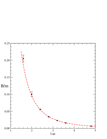
Figure 8: Binding energy versus lattice size $L$, for $g_{L}=0.3$, $\kappa=0.118$, and $a\mu=0.1$ averaged over 4000 samples for $L=16,\cdots,32$, 2000 for $L=36$, and 800 for $L=48$. Dotted line corresponds to a $1/L^{3}$ fit.

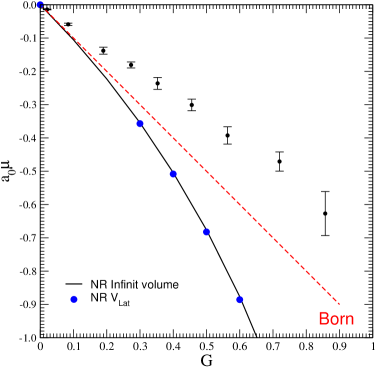
Figure 9: Scattering length vs $G$ for a lattice volume $La\mu=2.4$. Solid line indicates the continuum non-relativistic result and the dotted one the Born approximation (9). Blue circles represent the NR results.

In absence of bound states in the quenched approximation, we still can access to the NN low energy scattering parameters. The scattering observables cannot be obtained in Euclidean time in the infinite volume limit [46] but can be extracted from the volume dependent binding energy measured on finite lattices, like for instance the one plotted in Fig. 9. The underlying formalism was developed by Luscher in [47] who gave a $1/L$ expansion of the binding energy. In its leading order it reads:

$$\frac{B}{m}=-\frac{4\pi a_{0}\mu}{\left(\frac{m}{\mu}\right)^{2}(La\mu)^{3}}$$ (38)

Using the binding energy values of Fig. 9 and equation (38), the NN scattering lengths $a_{0}$ can be computed. The result – corresponding to $g_{L}=0.3$, $\kappa=0.118$, and $a\mu=0.1$ – is $a_{0}\mu\approx-0.13$ and the dimensionless coupling constant of the non-relativistic model is $G=0.193$. The corresponding non-relativistic scattering length value, given by Fig. 4, is $A_{0}=a_{0}\mu=-0.214$.

This study has been performed for several values of $g_{L}$. The dependence of $a_{0}$ on the coupling constant $G$ is plotted in Fig. 9, for a lattice size of $La\mu=2.4$ ($L=24$, $a\mu=0.1$). One can see that the lattice results notably departs from the non-relativistic ones (solid line) and are above the Born approximation (dashed line).

The values of the accessible coupling constants extend beyond the Born regime but are still far from the pole behavior corresponding to the appearance of the first bound state displayed in Fig. 4. The difference between the lattice and NR results may indicate strong repulsive corrections. These kind of corrections were already manifested in the bound state problem when solving the same Yukawa model both in Light Front and BS ladder equations.

5 Conclusion

We have presented the results of the Yukawa model for the NN system using three different dynamical frameworks. In this model – which constitutes the simplest renormalizable quantum field theory of a fermion-meson interaction – two fermions of identical mass $m$ interact by exchanging a massive scalar particle of mass $\mu$. Results are restricted to the $J^{\pi}=0^{+}$ state.

In non-relativistic dynamics the model consists in solving the Schrodinger equation with the so called – static and local – Yukawa potential (4). The results depend on three parameters ($m,\mu,g$) but some simple scaling properties make it dependent on a single dimensionless parameter, the coupling constant $G=(g^{2}/4\pi)(m/\mu)$. The existence of a first bound state requires the coupling constant to be greater than a critical value $G_{0}=1.680$. For $G>G_{0}$, its binding energy increases monotonously and can reach any arbitrary value, even greater than $2m$.

The way for implementing relativistic dynamics in the description of the same system is not unique. We have considered two relevant relativistic equations: Light-Front and Bethe-Salpeter. In both cases, for this particular coupling and state, the corresponding equations can be integrated without introducing any regularization form factor. The scaling properties of the non-relativistic model model are now lost and both equations exhibit a critical coupling constant $g_{c}$, for which $M^{2}$ tends to $-\infty$. For slightly smaller value of $g$ the mass $M^{2}$ crosses zero: the system ”collapses”. The precise numerical value of $g_{c}$ depends however on the particular dynamical framework: $g_{c}=6.84$ for Light-Front equation and $g_{c}=2\pi$ for BS one. This value is however large enough to generate several bound states. The corresponding relativistic binding energies $B(g^{2})$ are close to each other but they depart sizeably from the non-relativistic ones even for very loosely bound states and are strongly repulsive.

Relativistic equations are the first step towards a full Quantum Field Theory solution. They suffer from two main drawbacks. On one hand, most of the one-boson exchange kernels require to be regularized in order to obtain an integrable equation. This is usually done by introducing a vertex form factor cutting the high momentum components above some arbitrary value $\Lambda$, but thus diluting all the benefit of an approach starting from the first principles, like underlying Lagrangian. The Yukawa model (in $J=0^{+}$ state) is rather an exception than the generic case of one-boson exchange models. On the other hand, the ladder kernel accounts only for a small part of the interaction, specially when large values of the coupling constant are involved. We have presented the first attempt to incorporate the full dynamical content of the Yukawa model by using standard lattice techniques developed in the context of QCD.

The only approximation in the calculations was to neglect the N̄N loops (quenched approximation) as it is the case in all the nuclear models. The lattice results indicate the existence of a maximal coupling constant $g_{L}$ which is well below the required value for the existence of the first bound state in the heory. For smaller coupling constant the scattering length has been computed using Luscher’s prescription. Results are in agreement with the repulsive effect found by solving the relativistic equations.

We have shown how the same interaction model between fermions can give rise to very different physical pictures depending on the particular dynamical framework in which it is considered. The differences between a relativistic and a non-relativistic approach are not only quantitative but lead to new qualitative behavior. In the particular case of the Yukawa model, which was the first of all the nucleon-nucleon models, the full quantum field solution remains still unknown.

References

- [1] Bakamjian, B., Thomas, L.H.: Relativistic Particle Dynamics. II. Phys. Rev. 92, 1300-1310, (1953)
- [2] Keister, B.D., Polyzou, W.N.: Adv. in Nucl. Phys. 20, 225 (1991)
- [3] Yukawa, H.: On the Interaction of Elementary Particles. Proc. Math. Soc. Jap. 17, 48 (1935)
- [4] Salpeter, E.E., Bethe, H.: A Relativistic equation for bound state problems. Phys.Rev. 84, 1232-1242 (1951)
- [5] Gell-Mann, M., Low, F.: Bound states in quantum field theory. Phys. Rev. 84, 350-354 (1951)
- [6] Carbonell, J., Desplanques, B., Karmanov, V.A., Mathiot, J.-F.: Explicitly covariant light front dynamics and relativistic few body systems. Phys. Rept. 300, 215-347 (1998)
- [7] Dorkin, S., Beyer, M., Semikh, S., Kaptari, L.: Two-Fermion Bound States within the Bethe-Salpeter Approach. Few-Body Syst. 42, 1-32 (2008)
- [8] Dorkin, S., Kaptari, L., C. C. degli Atti, Kampfer, B.: Solving the Bethe-Salpeter Equation in Euclidean Space. Few-Body Syst. 49, 233-246 (2011)
- [9] Carbonell, J., Karmanov, V.A.: Solutions of the Bethe-Salpeter equation in Minkowski space and applications to electromagnetic form factors. Few-Body Syst. 49, 205-222 (2011)
- [10] Carbonell, J., Karmanov, V.A.: Solving Bethe-Salpeter equation for two fermions in Minkowski space. Eur. Phys. J. A 46, 387-397 (2010)
- [11] Fleischer, J., Tjon, J.A.: Nucl. Phys. B 84, 375 (1975)
- [12] Fleischer, J., Tjon, J.A.: Bethe-Salpeter Equation for I=1 Nucleon-Nucleon Scattering with One Boson Exchange. Phys.Rev. D 15, 2537-2546 (1977)
- [13] Fleischer, J., Tjon, J.A.: Bethe-Salpeter equation for elastic Nucleon Nucleon scattering. Phys. Rev. D 21, 87-94 (1980)
- [14] Karmanov, V.A., Carbonell, J.: Solution of Bethe-Salpeter Equation in Minkowski space for the Scattering States. Light Cone Meeting, 8-13 July, 2012, Cracow, Poland; to appear in Acta Phys. Polonica.
- [15] Karmanov, V.A., Carbonell, J.: Solving Bethe-Salpeter equation for scattering states. Presented at 20th International Conference on Few-Body Problems in Physics, 20 - 25 August, 2012, Fukuoka, Japan; to appear in Few-Body Syst., arXiv:1210.0925 [hep-ph]
- [16] Karmanov, V.A., Carbonell, J.: Scattering states in Bethe-Salpeter equation. Presented at XXI International Baldin Seminar on High Energy Physics Problems, 10-15 September 2012, Dubna, Russia; to appear in PoS.
- [17] Glazek, St., Harindranath, A., Pinsky, S., Shigemutsu, J., and Wilson, K.: Relativistic bound-state problem in the light-front Yukawa model. Phys. Rev. D 47, 1599-1619 (1993)
- [18] Glazek, St. and Wilson, K.G.: Renormalization of overlapping transverse divergences in a model light-front Hamiltonian. Phys. Rev. D 47, 4657-4669 (1993)
- [19] Mangin-Brinet, M., Carbonell, J., Karmanov, V.A.: Stability of bound states in the light front Yukawa model. Phys.Rev. D 64, 027701 (2001)
- [20] Mangin-Brinet, M., Carbonell, J., Karmanov, V.A.: Relativistic bound states in Yukawa model. Phys. Rev. D 64, 125005 (2001)
- [21] Karmanov, V.A., Carbonell, J., Mangin-Brinet, M.: Stability of bound states in the light front Yukawa model, AIP Conf.Proc. 603, 271-274 (2001)
- [22] Mangin-Brinet, M., Carbonell, J., Karmanov, V.A.: Stability of two fermion bound states in the explicitly covariant light front dynamics. Nucl. Phys. Proc. Suppl. 108, 259-263 (2002)
- [23] Karmanov, V.A., Carbonell, J., Mangin-Brinet, M., Two fermion bound states in the explicitly covariant light front dynamics. Nucl. Phys. Proc. Suppl. 108, 256-258 (2002)
- [24] Mangin-Brinet, M., Carbonell, J., Karmanov, V.A.: Two fermion relativistic bound states in light front dynamics. Phys. Rev. C 68, 055203 (2003)
- [25] Schoonderwoerd, N.C.J., Bakker, B.L.G. and Karmanov, V.A.: Entanglement of Fock-space expansion and covariance in light-front Hamiltonian dynamics. Phys. Rev. C 58, 3093-3108 (1998)
- [26] Ji, C.-R., Surya, Y.: Calculation of scattering with the light cone two-body equation in theories. Phys. Rev. D 46, 3565-3575 (1992)
- [27] Oropeza, D: Thèse Univ. Grenoble (2004), http://tel-ujf.ujf-grenoble.fr/
- [28] Levine, M., Tjon, J.A., Wright, J: Nonsingular Bethe-Salpeter Equation. Phys. Rev. Lett. 16, 962-964 (1966)
- [29] Levine, M., Wright, J., Tjon, J.A.: Solution of the Bethe-Salpeter Equation in the Inelastic Region. Phys. Rev. 154, 1433-1437 (1967)
- [30] Karmanov, V.A., Maris, P.: Three-body forces in Bethe-Salpeter and light-front equations, PoS LC2008 (2008) 037.
- [31] Karmanov, V.A., Maris, P.: Manifestation of three-body forces in three-body Bethe-Salpeter and light-front equations. Few-Body Syst. 46, 95-113 (2009)
- [32] Polyzou, W., Huang, Y., Elster, C., Glöckle, W., Golak, J.: et al.: Mini review of Poincaré invariant quantum theory. Few-Body Syst. 49, 129-147 (2011)
- [33] Kamada, H., Glöckle, W.: A Momentum transformation connecting a N N potential in the nonrelativistic and the relativistic two nucleon Schrodinger equation. Phys. Rev. Lett. 80, 2547-2549 (1998)
- [34] Witala, H., Golak, J., Skibinski, R.: Selectivity of the nucleon induced deuteron breakup and relativistic effects. Phys. Lett. B 634, 374-377 (2006)
- [35] Lin, T., Elster, C., Polyzou, W., Glöckle, W.: First Order Relativistic Three-Body Scattering. Phys. Rev. C 76, 014010 (2007)
- [36] Stadler, A., Gross, F.: Relativistic Calculation of the Triton Binding Energy and Its Implications. Phys. Rev. Lett. 78, 26-29 (1997); High-precision covariant one-boson-exchange potentials for np scattering below 350 MeV. Phys. Lett. B 657, 176-179 (2007)
- [37] Kamada, H., Glöckle, W.: Realistic two-nucleon potentials for the relativistic two-nucleon Schrodinger equation. Phys. Lett. B 655, 119-125 (2007)
- [38] Elster, C., Lin, T., Polyzou, W., Glöckle, W.: Poincare Invariant Three-Body Scattering. Few-Body Syst. 45, 157-160 (2009)
- [39] Witala, H., Golak, J., Skibinski, R., Glöckle, W., Polyzou, W. et al., Relativistic effects in 3N reactions. Mod. Phys. Lett. A 24, 871-874 (2009)
- [40] Carbonell, J., Karmanov, V.A.: Cross-ladder effects in Bethe-Salpeter and light-front equations. Eur. Phys. J. A 27, 11–21 (2006)
- [41] Nieuwenhuis, T, Tjon, J.A.: Nonperturbative study of generalized ladder graphs in a theory. Phys. Rev. Lett. 77, 814-817 (1996)
- [42] De Soto, F., Carbonell, J., Roiesnel, C., Boucaud, P., Leroy, J., et al.: Nuclear models on a lattice. Nucl. Phys. Proc. Suppl. 164, 252-255 (2007)
- [43] De Soto, F., Carbonell, J., Roiesnel, C., Boucaud, P., Leroy, J., et al.: Yukawa model on a lattice: Two body states. Eur. Phys. J. A 31, 777–780 (2007)
- [44] De Soto, F., Carbonell, J., Roiesnel, C., Boucaud, P., Leroy, J., et al.: Two body scattering length of Yukawa model on a lattice. Nucl. Phys. A 790. 410-413 (2007)
- [45] De Soto, F., Angles d’Auriac, J. C., Carbonell, J.: The Nuclear Yukawa Model on a Lattice. Eur. Phys. J. A 47, 57 (2011)
- [46] Maiani, L., Testa, M.: Final state interactions from euclidean correlation functions. Phys. Lett. B 245, 585-590 (1990)
- [47] Luscher, M.: Commun. Math. Phys. 104, 177 (1986); 105, 153 (1986)