Squiral Diffraction

Abstract

The Thue-Morse system is a paradigm of singular continuous diffraction in one dimension. Here, we consider a planar system, constructed by a bijective block substitution rule, which is locally equivalent to the squiral inflation rule. For balanced weights, its diffraction is purely singular continuous. The diffraction measure is a two-dimensional Riesz product that can be calculated explicitly.

1 Introduction

The diffraction of crystallographic structures and of aperiodic structures based on cut and project sets (or model sets) is well understood; see BaaGri-BG11 ; BaaGri-BG12a and references therein. These systems (in the case of model sets under suitable assumptions on the window) are pure point diffractive, and the diffraction can be calculated explicitly.

The picture changes for structures with continuous diffraction. Not much is known in general, in particular for the case of singular continuous diffraction, even though both absolutely and singular continuous diffraction show up in real systems BaaGri-WW ; BaaGri-W . The paradigm of singular continuous diffraction is the Thue-Morse chain, which in its balanced form (constructed via the primitive inflation rule $1\mapsto 1\bar{1}$, $\bar{1}\mapsto\bar{1}1$ with with weights $1$ and $\bar{1}=-1$, say) shows purely singular continuous diffraction. This was shown by Kakutani BaaGri-Kaku , see also BaaGri-BG08 , and the result can be extended to an entire family of generalised Thue-Morse sequences BaaGri-BGG12 .

Here, we describe a two-dimensional system which, in its balanced form, has purely singular continuous diffraction. For more detail and mathematical proofs, we refer to BaaGri-BG12b . Again, it is possible to obtain an explicit formula for the diffraction measure in terms of a Riesz product, with convergence in the vague topology.

2 The squiral block inflation

The squiral tiling (a name that comprises ‘square’ and ‘spiral’) was introduced in (BaaGri-GS, , Fig. 10.1.4) as an example of an inflation tiling with prototiles comprising infinitely many edges. The inflation rule is shown in Fig. 1; it is compatible with reflection symmetry, so that the reflected prototile is inflated accordingly.

[width=0.35]BaaGri-squiralinfl.eps

Figure 1: The primitive inflation rule for the squiral tiling of the Euclidean plane.

A patch of the tiling is shown in Fig. 2. Clearly, the tiling consists of a two-colouring of the square lattice, with each square comprising four squiral tiles of the same chirality. The two-colouring can be obtained by the simple block inflation rule sown in Fig. 3, which is bijective in the sense of BaaGri-Nat . Again, the rule is compatible with colour exchange. The corresponding hull has $D_{4}$ symmetry, and also contains an element with exact individual $D_{4}$ symmetry; see BaaGri-BG12b for details and an illustration.

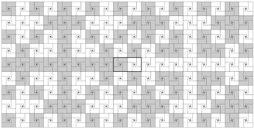
Figure 2: Patch of the squiral tiling obtained by two inflation steps from the central seed.

[width=0.5]BaaGri-sqblockinfl.eps

Figure 3: Equivalent block inflation rule for the squiral tiling of Figure 2.

Due to the dihedral symmetry of the inflation tiling, it suffices to consider a tiling of the positive quadrant. Using the lower left point of the square as the reference point, the induced block inflation $\varrho$ produces a two-cycle of configurations $v$ and $\varrho v$. They satisfy, for all $m,n\geq 0$ and $0\leq r,s\leq 2$, the fixed point equations

$$(\varrho v)_{3m+r,3n+s}\,=\,\cases{\overline{v}_{m,n},\quad\rm{if}\;r\equiv s\equiv 0\bmod 2,\cr v_{m,n},\quad\rm{otherwise}.}$$ (1)

3 Autocorrelation and diffraction measure

For a fixed point tiling under $\varrho^{2}$, we mark each (coloured) square by a point at its lower left corner $z\in\mathbb{Z}^{2}$. For the balanced version, each point carries a weight $w_{z}=1$ (for white) or $w_{z}=\bar{1}=-1$ (for grey). Consider the corresponding Dirac comb

$$\omega\,=\,w\,\delta_{\mathbb{Z}^{2}}\,=\sum_{z\in\mathbb{Z}^{2}}w_{z}\,\delta_{z}\,.$$ (2)

Following the approach pioneered by Hof BaaGri-Hof , the natural autocorrelation measure $\gamma$ of $\omega$ is defined as

$$\vspace*{-1mm}\gamma\,=\,\omega\circledast\widetilde{\omega}\,:=\,\lim_{N\to\infty}\frac{\bigl{(}\omega\big{|}_{C_{N}}\bigr{)}*\bigl{(}\widetilde{\omega\big{|}_{C_{N}}}\bigr{)}}{(2N+1)^{2}}\,,$$ (3)

where $C_{N}$ stands for the closed centred square of side length $2N$. Here, $\widetilde{\mu}$ denotes the measure defined by $\widetilde{\mu}(g)=\overline{\mu(\widetilde{g})}$ for $g\in C_{\mathsf{c}}(\mathbb{R}^{2})$, with $\widetilde{g}(x):=\overline{g(-x)}$ (and where the bar denotes complex conjugation). The autocorrelation measure $\gamma$ is of the form $\gamma=\eta\delta_{\mathbb{Z}^{2}}$ with autocorrelation coefficients

$$\eta(m,n)\,=\,\lim_{N\to\infty}\frac{1}{(2N+1)^{2}}\sum_{k,\ell=-N}^{N}w_{k,\ell}\,w_{k-m,\ell-n}\,.$$ (4)

All limits exists due to the unique ergodicity of the underlying dynamical system BaaGri-BG12b , under the action of the group $\mathbb{Z}^{2}$.

Clearly, one has $\eta(0,0)=1$, while Eq. (1) implies the nine recursion relations

$$\eta(3m,3n)\, = \,\eta(m,n)\,,$$

$$\eta(3m,3n\!+\!1)\, = \,-\textstyle\frac{2}{9}\eta(m,n)+\frac{1}{3}\eta(m,n\!+\!1)\,,$$

$$\eta(3m,3n\!+\!2)\, = \,\textstyle\frac{1}{3}\eta(m,n)-\frac{2}{9}\eta(m,n\!+\!1)\,,$$

$$\eta(3m\!+\!1,3n)\, = \,-\textstyle\frac{2}{9}\eta(m,n)+\frac{1}{3}\eta(m\!+\!1,n)\,,$$

$$\eta(3m\!+\!1,3n\!+\!1)\, = \,-\textstyle\frac{2}{9}\bigl{(}\eta(m\!+\!1,n)+\eta(m,n\!+\!1)\bigr{)}+\frac{1}{9}\eta(m\!+\!1,n\!+\!1)\,,$$ (5)

$$\eta(3m\!+\!1,3n\!+\!2)\, = \,-\textstyle\frac{2}{9}\bigl{(}\eta(m,n)+\eta(m\!+\!1,n\!+\!1)\bigr{)}+\frac{1}{9}\eta(m\!+\!1,n)\,,$$

$$\eta(3m\!+\!2,3n)\, = \,\textstyle\frac{1}{3}\eta(m,n)-\frac{2}{9}\eta(m\!+\!1,n)\,,$$

$$\eta(3m\!+\!2,3n\!+\!1)\, = \,-\textstyle\frac{2}{9}\bigl{(}\eta(m,n)+\eta(m\!+\!1,n\!+\!1)\bigr{)}+\frac{1}{9}\eta(m,n\!+\!1)\,,$$

$$\eta(3m\!+\!2,3n\!+\!2)\, = \,\textstyle\frac{1}{9}\eta(m,n)-\frac{2}{9}\bigl{(}\eta(m\!+\!1,n)+\eta(m,n\!+\!1)\bigr{)},$$

which hold for all $m,n\in\mathbb{Z}$ and determine all coefficients uniquely BaaGri-BG12b . The autocorrelation coefficients show a number of remarkable properties, which are interesting in their own right, and useful for explicit calculations.

Since the support of $\omega$ is the lattice $\mathbb{Z}^{2}$, the diffraction measure $\widehat{\gamma}$ is $\mathbb{Z}^{2}$-periodic BaaGri-B02 , and can thus be written as

$$\widehat{\gamma}\,=\,\mu*\delta_{\mathbb{Z}^{2}}\,,$$

where $\mu$ is a positive measure on the fundamental domain $\mathbb{T}^{2}=[0,1)^{2}$ of $\mathbb{Z}^{2}$. One can now analyse $\widehat{\gamma}$ via the measure $\mu$, which, via the Herglotz-Bochner theorem, is related to the autocorrelation coefficients by Fourier transform

$$\eta(k)\,=\,\int_{\mathbb{T}^{2}}e^{2\pi\mathrm{i}kz}\,\mathrm{d}\mu(z)\,,$$

where $k=(m,n)\in\mathbb{Z}^{2}$ and $kz$ denotes the scalar product. We now sketch how to determine the spectral type of $\mu$, and how to calculate it.

Defining $\Sigma(N)\,:=\,\sum_{m,n=0}^{N-1}\eta(m,n)^{2}$, the recursions (3) lead to the estimate

$$\Sigma(3N)\,\leq\,\frac{319}{81}\,\Sigma(N)\,,$$

so that $\Sigma(N)/N^{2}\longrightarrow 0$ as $N\to\infty$. An application of Wiener’s criterion in its multidimensional version BaaGri-BG12b ; BaaGri-TAO implies that $\mu$, and hence also the diffraction measure $\widehat{\gamma}$, is continuous, which means that it comprises no Bragg peaks at all.

Since $\eta(0,1)=\eta(1,0)=-1/3$, which follows from Eq. (3) by a short calculation, the first recurrence relation implies that $\eta(0,3^{j})=\eta(3^{j},0)=-1/3$ for all integer $j\geq 0$. Consequently, the coefficients cannot vanish at infinity. Due to the linearity of the recursion relations, the Riemann-Lebesgue lemma implies BaaGri-BG12b that $\mu$ cannot have an absolutely continuous component (relative to Lebesgue measure). The measure $\mu$, and hence $\widehat{\gamma}$ as well, must thus be purely singular continuous.

4 Riesz product representation

Although the determination of the spectral type of $\widehat{\gamma}$ is based on an abstract argument, the recursion relations (3) hold the key to an explicit, iterative calculation of $\mu$ (and hence $\widehat{\gamma}\>$). One defines the distribution function $F(x,y):=\mu\bigl{(}[0,x]\times[0,y]\bigr{)}$ for rectangles with $0\leq x,y<1$, which is then extended to the positive quadrant as

$$F(x,y)\,=\,\widehat{\gamma}\bigl{(}[0,x]\times[0,y]\bigr{)}.$$

This can finally be extended to $\mathbb{R}^{2}$ via $F(-x,y)=F(x,-y)=-F(x,y)$ and hence $F(-x,-y)=F(x,y)$. In particular, one has $F(0,0)=0$ as well as $F(0,y)=F(x,0)=0$, and $F$ is continuous on $\mathbb{R}^{2}$. The latter property is non-trivial, and follows from the continuity of certain marginals; see BaaGri-BG12b and references therein for details.

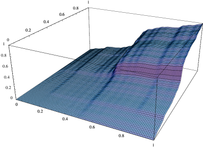
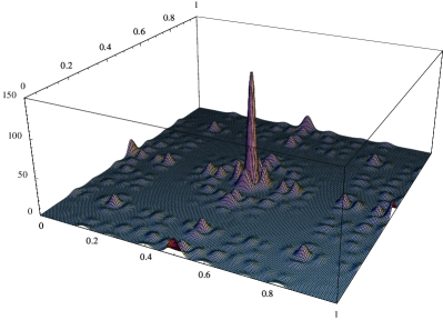
Figure 4: The distribution function $F^{(3)}$ of Eq. (7) (left) and the corresponding density $f^{(3)}$ of Eq. (8) (right), approximating the diffraction measure $\widehat{\gamma}$ of the squiral tiling on $[0,1]^{2}$.

One can show that, as a result of Eq. (3), $F$ satisfies the functional relation

$$F(x,y)\,=\,\frac{1}{9}\int_{0}^{3x}\int_{0}^{3y}\vartheta\bigl{(}\frac{x}{3},\frac{y}{3}\bigr{)}\,\mathrm{d}F(x,y)\,,$$ (6)

written in Lebesgue-Stieltjes notation, with the trigonometric kernel function

$$\vartheta(x,y)\,=\,\frac{1}{9}\bigl{(}1+2\cos(2\pi x)+2\cos(2\pi y)-4\cos(2\pi x)\cos(2\pi y)\bigr{)}^{2}.$$

The functional relation (6) induces an iterative approximation of $F$ as follows. Starting from $F^{(0)}(x,y)=xy$ (which corresponds to Lebesgue measure, $\mathrm{d}F^{(0)}=\lambda$) and continuing with the iteration

$$F^{(N+1)}(x,y)\,=\,\frac{1}{9}\int_{0}^{3x}\int_{0}^{3y}\vartheta\bigl{(}\frac{x}{3},\frac{y}{3}\bigr{)}\,\mathrm{d}F^{(N)}(x,y)\,,$$ (7)

one obtains a uniformly (but not absolutely) converging sequence of distribution functions, each of which represents an absolutely continuous measure. With $\mathrm{d}F^{(N)}(x,y)=f^{(N)}(x,y)\,\mathrm{d}x\,\mathrm{d}y$, where $f^{(N)}(x,y)\,=\,\frac{\partial^{2}}{\partial x\ts\partial y}F^{(N)}(x,y)$, one finds the Riesz product

$$f^{(N)}(x,y)\,=\prod_{\ell=0}^{N-1}\vartheta(3^{\ell}x,3^{\ell}y)\,.$$ (8)

These functions of increasing ‘spikiness’ represent a sequence of (absolutely continuous) measures that converge to the singular continuous squiral diffraction measure in the vague topology. The case $N=3$ is illustrated in Figure 4. Local scaling properties can be derived from Eq. (8).

5 Summary and outlook

The example of the squiral tiling demonstrates that the constructive approach of Refs. BaaGri-Kaku ; BaaGri-BG08 ; BaaGri-BGG12 can be extended to more than one dimension. The result is as expected, and analogous arguments apply to a large class of binary block substitutions that are bijective in the sense of BaaGri-Nat . This leads to a better understanding of binary systems with purely singular continuous diffraction.

It is desirable to extend this type of analysis to substitution systems with larger alphabets. Although the basic theory is developed in BaaGri-Q , there is a lack of concretely worked-out examples. Moreover, there are various open questions in this direction, including the (non-)existence of bijective constant-length substitutions with absolutely continuous spectrum (the celebrated example from (BaaGri-Q, , Ex. 9.3) was recently recognised to be inconclusive by Alan Bartlett and Boris Solomyak).

- (1) Baake, M., Grimm, U.: The singular continuous diffraction measure of the Thue-Morse chain. J. Phys. A.: Math. Theor. 41, 422001 (6pp) (2008); arXiv:0809.0580.
- (2) Baake, M.: Diffraction of weighted lattice subsets. Can. Math. Bulletin 45, 483–498 (2002); arXiv:math.MG/0106111.
- (3) Baake, M., Gähler, F., Grimm, U.: Spectral and topological properties of a family of generalised Thue-Morse sequences. J. Math. Phys. 53, 032701 (24pp) (2012); arXiv:1201.1423.
- (4) Baake, M., Grimm, U.: Kinematic diffraction from a mathematical viewpoint. Z. Kristallogr. 226, 711–725 (2011); arXiv:1105.0095.
- (5) Baake, M., Grimm, U.: Mathematical diffraction of aperiodic structures. Chem. Soc. Rev. 41, 6821–6843 (2012); arXiv:1205.3633.
- (6) Baake, M., Grimm, U.: Squirals and beyond: Substitution tilings with singular continuous spectrum. Ergodic Th. & Dynam. Syst., to appear; arXiv:1205.1384 (2012).
- (7) Baake, M., Grimm, U.: Theory of Aperiodic Order: A Mathematical Invitation, Cambridge University Press, Cambridge, to appear (2013).
- (8) Grünbaum, B., Shephard, G.C.: Tilings and Patterns. Freeman, New York (1987).
- (9) Hof, A.: On diffraction by aperiodic structures. Commun. Math. Phys. 169, 25–43 (1995).
- (10) Kakutani, S.: Strictly ergodic symbolic dynamical systems. In: LeCam, L.M., J Neyman, J., and E L Scott, E.L. (eds.) Proc. 6th Berkeley Symposium on Math. Statistics and Probability, pp. 319–326. Univ. of California Press, Berkeley (1972).
- (11) Frank N.P.: Multi-dimensional constant-length substitution sequences, Topol. Appl. 152, 44–69 (2005).
- (12) Queffélec M.: Substitution Dynamical Systems – Spectral Analysis, LNM 1294, 2nd ed., Springer, Berlin (2010).
- (13) Welberry, T.R., Withers, R.L.: The rôle of phase in diffuse diffraction patterns and its effect on real-space structure. J. Appl. Cryst. 24, 18–29 (1991).
- (14) Withers, R.L.: Disorder, structured diffuse scattering and the transmission electron microscope. Z. Kristallogr. 220, 1027–1034 (2005).