Remote synchronization reveals network symmetries and functional modules

Abstract

We study a Kuramoto model in which the oscillators are associated with the nodes of a complex network and the interactions include a phase frustration, thus preventing full synchronization. The system organizes into a regime of remote synchronization where pairs of nodes with the same network symmetry are fully synchronized, despite their distance on the graph. We provide analytical arguments to explain this result and we show how the frustration parameter affects the distribution of phases. An application to brain networks suggests that anatomical symmetry plays a role in neural synchronization by determining correlated functional modules across distant locations.

Synchronization of coupled dynamical units is a ubiquitous phenomenon in nature piko . Remarkable examples include phase locking in laser arrays, rhythms of flashing fireflies, wave propagation in the heart, and also normal and abnormal correlations in the activity of different regions of the human brain strogatz ; bullmore ; chavez_brain ; Tass1999 . In 1975 Y. Kuramoto proposed a simple microscopic model to study collective behaviors in large populations of interacting elements kuramoto . In its original formulation the Kuramoto model describes each unit of the system as an oscillator which continuously readjusts its frequency in order to minimize the difference between its phase and the phase of all the other oscillators. This model has shown very successful in understanding the spontaneous emergence of synchronization and, over the years, many variations have been considered sakaguchi ; strogatzrev_kuramoto ; acebron . Recently, the Kuramoto model has been also extended to sets of oscillators coupled through complex networks strogatz ; watts ; rev:bocc , and it has been found that the topology of the interaction network has a fundamental role in the emergence and stability of synchronized states Wiley2006 ; PRsync . In particular, the presence of communities —groups of tightly connected nodes— has a relevant impact on the path to synchronization arenas_modules ; bocca_modules ; gardenes ; adaptive ; luce , and units that are close to each other on the network, or belong to the same module or community fortunato , have a higher chance to exhibit similar dynamics. This implies that nodes in the same structural module share similar functions, which is a belief often supported by empirical findings Tegner2003 ; bullmore . However, various examples are found in nature where functional similarity is instead associated with morphological symmetry. In these cases, units with similar roles, which could potentially swap their position without altering the overall functioning of the system, appear in remote locations of the network. Some examples include cortical areas in brains varela2001 , symmetric organs in plants and vertebrates Smith2006 ; Ruvinsky2000 , and even atoms in complex molecules Rosenthal1936 . Therefore, identifying the sets of symmetric units of a complex system might be helpful to understand its organization. Finding the global symmetries in a graph, i.e., constructing its automorphism group, is a classical problem in graph theory. However, it is still unknown if this problem is polynomial or NP-complete footnote1 ; Papadimitriou1994 , even if there exist polynomial-time algorithms for graphs with bounded maximum degree luks82 . Recent works have focused instead on defining and detecting local symmetries in complex networks holme1 ; holme2 . Nevertheless, the interplay between the structural symmetries of a network and the dynamics of processes occurring over the network has been studied only marginally Russo2011 ; remote ; Aufderheide2012 , or for specific small network motifs Fischer2006 ; Vicente2008 ; Viriyopase2012 .

In this Letter we show that network symmetries play a central role in the synchronization of a system. We consider networks of identical Kuramoto oscillators, in which a phase frustration parameter forces connected nodes to maintain a finite phase difference, thus hindering the attainment of full synchronization. We prove that the configuration of phases at the synchronized state reflects the symmetries of the underlying coupling network. In particular, two nodes with the same symmetry have identical phases, i.e., are fully synchronized, despite the distance between the two nodes on the graph. Such a remote synchronization behavior is here induced by the network symmetries and not by an initial ad hoc choice of different natural frequencies remote .

Let us consider $N$ identical oscillators associated to the nodes of a connected graph $G({\cal N},{\cal L})$, with $N=|{\cal N}|$ nodes and $K=|{\cal L}|$ links. Each node $i$ is characterized, at time $t$, by a phase $\theta_{i}(t)$ whose time evolution is governed by the equation

$$\dot{\theta}_{i}=\omega+\lambda\sum_{j=1}^{N}a_{ij}\sin(\theta_{j}-\theta_{i}-\alpha)\;.$$ (1)

Here $\omega$ is the natural frequency, identical for all the oscillators, and $A\equiv\{a_{ij}\}$ is the adjacency matrix of the coupling graph. The model has two control parameters: $\lambda>0$ accounting for the strength of the interaction, and $\alpha$, the phase frustration parameter ranging in $[0,\pi/2]$. When $\alpha=0$, the model reduces to a network of identical Kuramoto oscillators. In this case, the fully synchronized state is globally stable for a set of initial conditions having finite measure kuramoto ; acebron and the transient dynamics closely reflects the structure of the graph, so that nodes belonging to the same structural module evolve similarly in time arenas_modules . However, the synchronized state can coexist with other nontrivial attractors, e.g., uniformly twisted waves, especially if the coupling topology is regular and sparse (see Ref. Wiley2006 for a discussion about the size of the sync basin). Instead, if the oscillators are not identical the frequency distribution tends to separate their phases and, as a result, there is a transition from an incoherent state (with order parameter $r=\frac{1}{N}\left|\sum_{j=1}^{N}{\mbox{e}}^{i\theta_{j}}\right|$ equal to 0) to a synchronized one ($r\neq 0$) at a critical value $\lambda_{c}$ of the coupling strength.

The introduction of a phase frustration $\alpha\neq 0$ forces directly connected oscillators to maintain a constant phase difference nota . In particular, we found that for a wide range of $\alpha>0$ the dynamics in Eqs. (1) reaches a stationary state in which the oscillators at two symmetric nodes have exactly the same phase, and this phase differs from the phases of nodes with different symmetries. Let us first illustrate this behavior and the effect of $\alpha$ on the three graphs $G_{a}$, $G_{b}$ and $G_{c}$ shown in Fig. 1.

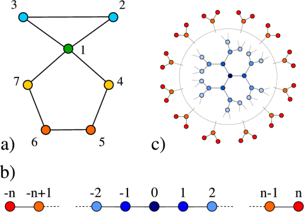
Figure 1: (color online) The presence of frustration reveals clusters of symmetric nodes. The color code represents the phases of nodes at a given time in the stationary state. (a) In the first graph ($G_{a}$), node 2 is synchronized to node 3, node 4 to node 7, and node 5 to node 6. (b) In a finite chain ($G_{b}$), pairs of nodes symmetrically placed with respect to the central node are perfectly synchronized. (c) In a finite Bethe lattice ($G_{c}$) all the nodes placed at the same distance from the center have equal phases.

In the three topmost panels of Fig. 2 we report the results of the numerical integration of Eqs. (1) on the graph $G_{a}$ for three different values of $\alpha$. We find that, after a transient, the system settles into a stationary state in which, at any time $t$, the phases are grouped into four different trajectories: $\theta_{1}(t)$, $\theta_{2}(t)=\theta_{3}(t)$, $\theta_{4}(t)=\theta_{7}(t)$ and $\theta_{5}(t)=\theta_{6}(t)$. In general, by increasing $\alpha$ up to a certain value $\alpha_{c}$ we better separate the four trajectories.

The four clusters of nodes obtained for $\alpha<\alpha_{c}$ are identified by a color code in Fig. 1. We notice that each cluster groups together all the nodes with the same symmetry. In this way two distant nodes of the graph, e.g. node $4$ and node $7$, are fully synchronized even if the other nodes in the paths connecting them have different phases. In this respect, what we observe is a remote synchronization remote . We have found similar results for the linear chain and for the Bethe lattice (see nodes with the same colors in $G_{b}$ and $G_{c}$ in Fig. 1).

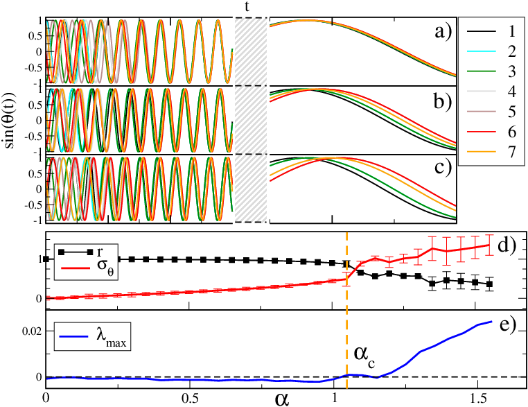
Figure 2: (color online) The figure refers to the coupling topology $G_{a}$ in Fig. 1a. Panels (a)–(c): after an initial transient the system reaches a phase-locked synchronized state in which symmetric nodes have the same phase. The panels correspond to three different values of the frustration parameter, respectively, (a) $\alpha=0.1$, (b) $\alpha=0.5$, (c) $\alpha=0.8$. Panel (d): for $\alpha>\alpha_{c}$ the synchronized state becomes unstable, the order parameter decreases while the dispersion of the phases $\sigma_{\theta}$ increases. Panel (e): the maximum Lyapunov exponent $\lambda_{max}$ of oscillators coupled through $G_{a}$ becomes positive for $\alpha>\alpha_{c}$, and the systems enters a chaotic regime. The dashed yellow line indicates the approximate position of $\alpha_{c}$.

Notice that if the system reaches a synchronized state and $\alpha$ is small enough, Eq. (1) can be linearized by replacing the sinus with its argument. We obtain

$$\dot{\theta}_{i}=\omega-\lambda\left[\sum_{j=1}^{N}L_{ij}\theta_{j}+\alpha k_{i}\right]~{}~{}$$ (2)

where $k_{i}=\sum_{j}a_{ij}$ is the degree of node $i$, $L_{ij}$ are the entries of the Laplacian matrix of the graph $L\equiv D-A$, and $D$ is a diagonal matrix such that $D_{ii}=k_{i}$. Without loss of generality, we can set $\lambda=1$, $\omega=0$. If the system is synchronized then $\dot{\theta_{i}}=\Omega,\forall i$, so that the phases must satisfy the equations $\sum_{j=1}^{N}L_{ij}\theta_{j}=\alpha\left[\langle k\rangle-k_{i}\right]$ at any time, or equivalently

$$L\bm{\theta}=\alpha\left[\langle k\rangle\bm{1}-\bm{k}\right]$$ (3)

where $\langle k\rangle=N^{-1}\sum_{i}k_{i}$ is the average degree of the network. This corresponds to a synchronization frequency $\dot{\theta}_{i}\!=\!\Omega\!=\!-\alpha\langle k\rangle\>\forall i$. In a connected graph the Laplacian matrix has one null eigenvalue and the system of Eqs. (3) is singular. Consequently, at each time $t$ we can solve the system by computing the phase difference between each node and a given node chosen as reference. For instance, if in $G_{a}$ we define $\phi_{j}(t)=\theta_{j}(t)-\theta_{1}(t),j=2,\ldots,7$, by solving Eqs. (3) we obtain $\phi_{2}=\phi_{3}=\alpha\left[\langle k\rangle-2\right]$, $\phi_{4}=\phi_{7}=2\alpha\left[\langle k\rangle-2\right]$, and $\phi_{5}=\phi_{6}=3\alpha\left[\langle k\rangle-2\right]$. This is in agreement with the results of the simulations: the phases are clustered into four groups, with nodes with the same symmetry having the same phase, and nodes with different symmetries being separated by a phase lag that depends on $\alpha$ as in the relations found above. An analogous analytical expression can be derived for a finite chain (graph $G_{b}$ in Fig.1), for which we obtain $\theta_{n}-\theta_{n-i}=\theta_{-n}-\theta_{-n+i}=\left[\frac{i(i+1)}{2}\langle k\rangle-i^{2}\right]\alpha$ and $\theta_{n}\!-\!\theta_{0}\!=\!\theta_{-n}\!-\!\theta_{0}\!=\!\left[\frac{n(n+1)}{2}\langle k\rangle-n^{2}\right]\alpha$. Consequently, two nodes symmetrically placed with respect to node $0$ will have identical phases.

We now provide a general argument to explain why the synchronization of Eqs. (1) is related to graph symmetries. A graph $G({\cal N},{\cal L})$ has a symmetry if and only if it is possible to find a bijection $\pi:{\cal N}\rightarrow{\cal N}$ which preserves the adjacency relation of $G$, i.e., which is an automorphism for $G$. Formally, this means that there exists a permutation matrix $P=P(\pi)$ such that $PAP^{-1}=A$. If $P$ corresponds to an automorphism of $G$ then $P$ commutes with $A$, i.e., $PA=AP$, and $PAP^{-1}$ performs a relabeling of the nodes of the original graph which preserves the adjacency matrix footnote2 . In general a graph can admit more than one automorphism. For instance, graph $G_{a}$ in Fig.1 has at least three nontrivial bijections which preserve the adjacency matrix, namely

$$\begin{array}[]{llcr}\pi_{1}&:(1,2,3,4,5,6,7)&\rightarrow&(1,3,2,4,5,6,7)\\ \pi_{2}&:(1,2,3,4,5,6,7)&\rightarrow&(1,2,3,7,6,5,4)\\ \pi_{3}&:(1,2,3,4,5,6,7)&\rightarrow&(1,3,2,7,6,5,4)\\ \end{array}$$

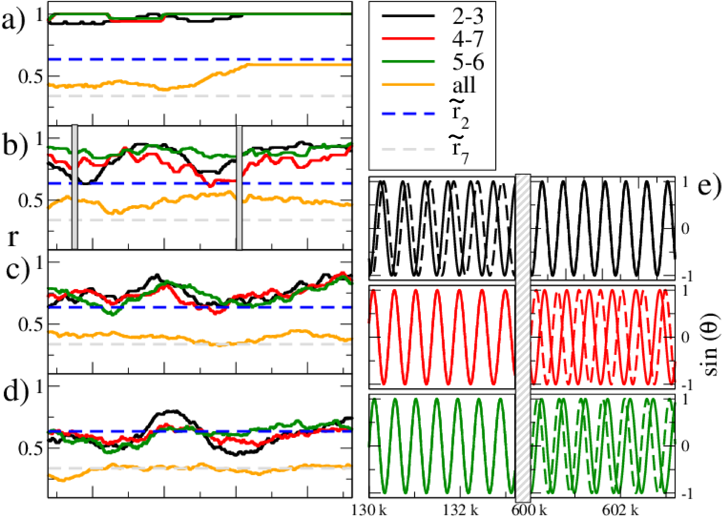
Figure 3: (color online) Chaotic regime in $G_{a}$ when $\alpha>\alpha_{c}$. Panel (a)–(d): running averages of $r$ (orange) and pairwise order parameters $r_{2}$ (black, red and green lines) for typical trajectories of oscillators coupled through graph $G_{a}$, when $\alpha$ is respectively equal to (a) $1.3$, (b) $1.4$, (c) $1.5$ and (d) $1.55$. The dashed lines indicate the expected synchronization level for a system of two (blue line, $\tilde{r_{2}}=2/\pi$) and seven incoherent oscillators (gray line, $\tilde{r_{7}}\simeq 0.338\ldots$). Panel (e) the plot of the phases of pairs of symmetric nodes for $\alpha=1.4$ in two different temporal intervals (the shaded gray regions in panel b) reveal the existence of metastable, partially synchronized states.

Node $2$ and node $3$ are symmetric because we can relabel the nodes of $G_{a}$ (e.g. by means of either $\pi_{1}$ or $\pi_{3}$) so that node $2$ is mapped into node $3$ and vice versa, and the adjacency matrix of $G_{a}$ is left unchanged. Similarly, for the pairs $\{4,7\}$ and $\{5,6\}$, there are two different relabelings which preserve adjacency relations, i.e., $\pi_{2}$ and $\pi_{3}$. In terms of symmetries, the graph $G$ has the following four different classes of nodes: $C_{1}=\{1\}$, $C_{2}=\{2,3\}$, $C_{3}=\{4,7\}$, $C_{4}=\{5,6\}$. Now, if a permutation of the nodes is an automorphism of $G$, then $PLP^{-1}=PDP^{-1}-PAP^{-1}=D-A=L$, i.e., the associated permutation matrix $P$ also commutes with the Laplacian matrix of the graph. By left-multiplying both sides of Eq. (3) by $P$, we get $PL\bm{\theta}=\alpha P\left[\langle k\rangle\bm{1}-\bm{k}\right]$. Since $PL=LP$ ($P$ commutes with $L$) and $P\bm{k}=\bm{k}$ (symmetric nodes have the same degree) then we have

$$LP\bm{\theta}=\alpha\left[\langle k\rangle\bm{1}-\bm{k}\right]$$ (4)

Combining Eq. (3) and Eq. (4) we finally obtain the linear system

$$LP\bm{\theta}=L\bm{\theta}$$ (5)

which is singular, i.e., has one free variable. Again, it can be solved by leaving free one of the $N$ variables $\theta_{i}$, setting $\phi_{j}=\theta_{j}-\theta_{i}$ and considering the new system $\tilde{L}\tilde{P}\bm{\phi}=\tilde{L}\bm{\phi}$. The matrix $\tilde{P}$ is obtained from $P$ by removing the row and the column corresponding to node $i$. If $P$ does not permute node $i$ with another node, then $\tilde{P}$ is still a permutation matrix. Similarly, $\tilde{L}$ is the reduced Laplacian, i.e., the matrix obtained from the Laplacian by deleting the $i-$th row and the $i-$th column. By left-multiplying by $\tilde{L}^{-1}$, which is not singular, we obtain

$$\tilde{P}\bm{\phi}=\bm{\phi}$$ (6)

Since $\tilde{P}\bm{\phi}$ is a permutation of the phases of symmetric nodes, Eq.(6) implies that the phases of symmetric nodes will be equal at any time, whereas by solving Eq. (4) we can get the values of the corresponding phases. This argument is valid for small values of $\alpha$, since the linearization of Eq. (1) is possible only if $\sin(x-\alpha)\simeq(x-\alpha)$, but as shown in Fig. 2(a)-(c) we observe the formation of the same perfectly synchronized clusters of symmetric nodes for a wide range of $\alpha$. However, when $\alpha$ becomes larger than a certain value $\alpha_{c}$, the assumption $\dot{\theta_{i}}=\Omega,\forall i$ does not hold any more and the global synchronized state loses stability. By looking at Fig. 2(d)-(e) we notice that for $\alpha>\alpha_{c}$, with $\alpha_{c}\simeq 1.05$ for the graph $G_{a}$, the value of $r$ steadily decreases while the dispersion of phases increases, until it reaches the expected value $\bar{\sigma}_{\theta}\simeq 1.39$ for a system of seven incoherent oscillators (see Fig. 2(d) and Appendix). Moreover, for $\alpha>\alpha_{c}$ the maximal Lyapunov exponent of the system $\lambda_{max}$ becomes positive and the system enters a chaotic regime (see Fig. 2(e)). Interestingly, the results reported in Fig. 3(a)-(d) confirm that in this regime the coherence of symmetric nodes, measured by the pairwise order parameter $r_{2}$, is higher than expected for incoherent oscillators (refer to Appendix for additional details). Figure 3(e) shows that for $\alpha>\alpha_{c}$ the system exhibits metastable, partially synchronized states, in which pairs of symmetric nodes alternates intervals of perfect synchronization with intervals of complete incoherence. We point out that in this regime chimera states could potentially occur chimera1 ; Laing2009 ; Shanahan2010 ; Martens2010 and could even coexist with remote synchronization for $\alpha<\alpha_{c}$. Qualitatively similar results are obtained for different coupling topologies, but the actual value of $\alpha_{c}$ seems to depend on the structure of the coupling network in a nontrivial way.

Application to the brain.– As an example, we investigate here the role of symmetry in the human brain by considering anatomical and functional brain connectivity graphs defined on the same set of $N=90$ cortical areas (see details in Appendix). We have first constructed a graph of anatomical brain connectivity as obtained from DW-MRI data iturria2011 , where links represent axonal fibers, and we used this graph as a backbone network to integrate Eqs. (1).

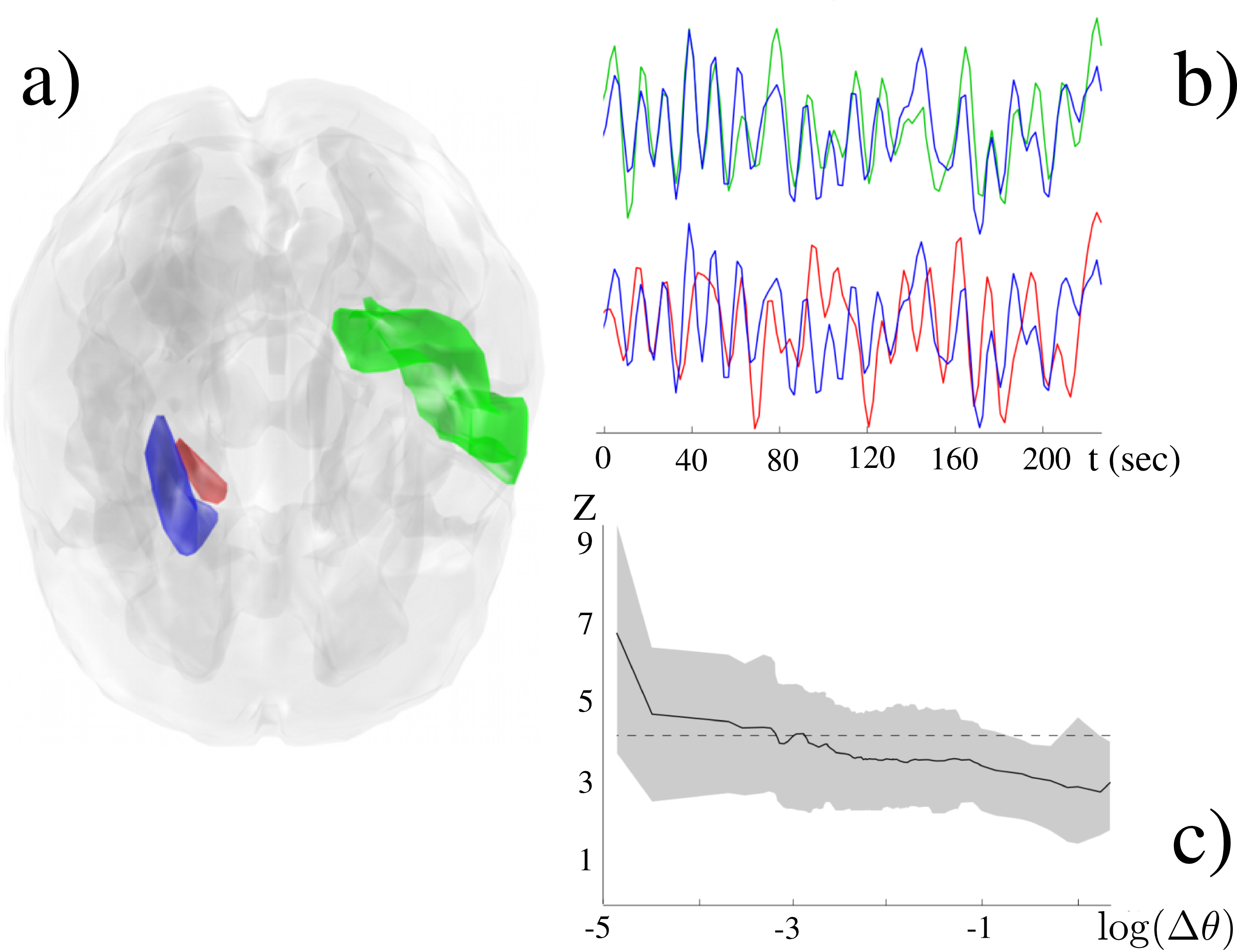
Figure 4: (color online) (a) Brain areas with similar and dissimilar phases of the frustrated Kuramoto model are colored and superimposed onto an anatomical image. (b) Examples of functional data from one subject recorded at the brain areas indicated in panel (a). Colors are the same as those used in the anatomical image. (c) Functional correlation $Z$ between pairs of nodes as a function of their phase differences $\Delta\theta$ according to the simulated Kuramoto dynamics. The black solid curve corresponds to the average value over all the subjects, while the gray area covers the $5^{\text{th}}$ and the $95^{\text{th}}$ percentiles of the distribution. The dashed horizontal line indicates the threshold for statistical significant correlations ($p<0.05$, corrected for multiple comparisons).

We identified candidate pairs of anatomically symmetric areas by means of agglomerative clustering, i.e., grouping together nodes having close phases at the stationary state (full dendrogram and details are provided in Appendix). Then, we considered the graph of functional brain connectivity, in which links represent statistically significant correlations between the BOLD fMRI time-series of cortical areas (see details in Appendix). Figure 4 illustrates the results for $\alpha=0.5$ (we obtained qualitatively similar results in a wide range of $\alpha$). Consider nodes 57 and 74, corresponding respectively to the green and blue areas in panel (a). Not only the two areas are spatially separated, but there is no edge connecting the two corresponding nodes in the anatomical connectivity network. However, the two nodes are detected as a candidate symmetric pair since at the stationary state of the Kuramoto dynamics in Eq. (1) the oscillators associated to these two nodes have very close phases (see dendrogram in Appendix). As shown in Fig. 4(b), also the BOLD fMRI signals corresponding to nodes 57 and 74 also are strongly synchronized. We obtain remarkably different results when we consider node 74 and node 76. These nodes correspond to two spatially adjacent areas of the brain (the red and blue regions in Fig. 4(a) and are directly connected in the anatomical connectivity network. However, at the stationary state of Eq. (1) the phase difference of the oscillators associated to node 74 and 76 is quite large. Interestingly, in this case the fMRI time-series associated to these nodes are much less similar to each other [see the two bottom trajectories reported in Fig. 4(b)].

To quantify this effect, we plot in Fig. 4c the average functional correlation $Z$ between the fMRI activity of pairs of brain areas as a function of the phase differences $\Delta\theta$ between the phases of the corresponding oscillators, obtained from the dynamics of Eq. (1) on the anatomical connectivity network. The fact that $Z$ decreases with $\Delta\theta$ suggests that structural symmetry plays an important role in determining human brain functions. In fact, the functional activities of anatomically symmetric areas can be strongly correlated, even if the areas are distant in space. These results suggest that the study of anatomical symmetries in neural systems might provide meaningful insights about the functional organization of distant neural assemblies during diverse cognitive or pathological states varela2001 . Applied to other connectivity networks as a method to spot potential network symmetries, our study could provide new insights on the interplay between structure and dynamics in complex systems.

Appendix

Expected order parameter for two incoherent oscillators. – In Fig.3 of the main text we showed that when $\alpha$ approaches $\pi/2$ the order parameter $r_{2}$ for a pair of symmetric oscillators remains higher than the expected value $\bar{r}_{2}$ for a pair of incoherent oscillators. We report here the derivation of $\bar{r}_{2}$ for a pair of oscillators that are not synchronized. We assume that the phases $\theta_{1}$ and $\theta_{2}$ of the two oscillators are drawn uniformly in $[0,2\pi]$. Thanks to the rotational symmetry, we can set one of the phases equal to $0$, e.g. $\theta_{1}=0$, while drawing the other uniformly in $[0,2\pi]$. We notice that the value of $r_{2}$ for the generic pair of phases $(\theta_{1}=0,\theta_{2})$ reads:

$$r_{2} = \frac{1}{2}\sqrt{\left(\cos{\theta_{1}}+\cos{\theta_{2}}\right)^{2}+\left(\sin{\theta_{1}}+\sin{\theta_{2}}\right)^{2}}=$$

$$= \frac{1}{2}\sqrt{\left(1+\cos{\theta_{2}}\right)^{2}+\sin^{2}{\theta_{2}}}=$$

$$= \frac{1}{2}\sqrt{2+2\cos{\theta_{2}}}$$

Consequently, the expected value of $r_{2}$ is obtained as the average over all the possible choices of $\theta_{2}$, namely:

$$\tilde{r_{2}} = \frac{1}{4\pi}\int_{-\pi}^{\pi}\sqrt{2+2\cos{\theta}}\,\mathrm{d}\theta=$$

$$= \frac{1}{\pi}\int_{-\pi/2}^{\pi/2}\cos{u}\,\mathrm{d}u=$$

$$= \frac{2}{\pi}\simeq 0.6366197\ldots$$

Phase dispersion and numerical estimate for incoherent oscillators. – In Fig.2d of the main text we reported, as a function of $\alpha$, the dispersion of the phases $\sigma_{\theta}$ for a system of seven oscillators coupled through graph $G_{a}$ in Fig.1a. We noticed that the dispersion approaches the value $1.39$ when $\alpha\rightarrow\pi/2$. Given a set of $N$ unitary vectors having phases $\{\theta_{1},\theta_{2},\ldots,\theta_{N}\}$, consider the average vector:

$$re^{\text{i}\psi}=\frac{1}{N}\sum_{j=1}^{N}e^{\text{i}\theta_{j}}$$ (S-1)

having polar coordinates $(r,\psi)$. The dispersion of the $N$ phases of the set around the phase $\psi$ of the average vector is defined as:

$$\sigma_{\theta}=\sqrt{\frac{1}{N}\sum_{j=1}^{N}(\theta_{j}-\psi)^{2}}$$ (S-2)

where the difference $(\theta_{j}-\psi$) is computed $\text{mod}(2\pi)$ and takes in $[0,\pi]$. An estimate of the expected phase dispersion for a set of $N$ incoherent oscillators can be obtained as the average over $M$ independent realizations of $\sigma_{\theta}$ computed on a set of $N$ phases uniformly drawn in $[0,2\pi]$. For the system of $N=7$ oscillators coupled through graph $G_{a}$ we averaged $\sigma_{\theta}$ over $M=10^{7}$ samples, obtaining the estimate $\bar{\sigma}_{\theta}=1.394\pm 0.248$.

Computation of the maximum Lyapunov exponent $\lambda_{max}$. – The computation of the maximum Lyapunov exponent for the system coupled through graph $G_{a}$ of Fig. (1) in the main text was performed using equally separated values of $\alpha$ between $0$ and $1.57\simeq\pi/2$ ($\Delta\alpha=0.01$). Then, for each value of $\alpha$, we considered 500 different initial configurations of the phases of the seven oscillators. For each initial condition, we let evolve the trajectory $\bm{\theta}(t)$ according to Eq. (1) in the main text, until it reached the attractor (or the stationary state, for $\alpha\ll\pi/2$). To properly take into account the rotational symmetry of the system, we studied the evolution of $\bm{\theta}(t)$ in Cartesian coordinates, i.e., by looking at the set of $2N$ variables $\bm{x}=\{\cos{\theta_{1}},\cos{\theta_{2}},\ldots,\cos{\theta_{N}},\sin{\theta_{1}},\sin{\theta_{2}},\ldots,\sin{\theta_{N}}\}$. We considered a perturbation of $\bm{x}$ of magnitude $\varepsilon=10^{-4}$, i.e., a trajectory $\tilde{\bm{x}}$ such that $d(\bm{x}(t),\tilde{\bm{x}}(t))=\varepsilon$. Here $d(\cdot,\cdot)$ denotes the Euclidean distance in $\mathbb{R}^{2N}$. Then, we integrated both trajectories for one integration step $h$ (using a standard fourth-order Runge-Kutta integration scheme), we measured the distance $d_{1}=d(\bm{x}(t+h),\tilde{\bm{x}}(t+h))$ and we computed $\lambda=\log{(d_{1}/\varepsilon)}$. The quantity $\lambda$ is a one-step approximation of the largest Lyapunov exponent of the system Strogatz1994a . Then, we realigned the perturbed trajectory $\tilde{\bm{x}}$ so that the distance between $\bm{x}(t+h)$ and the realigned perturbed trajectory $\tilde{\tilde{\bm{x}}}(t+h)$ was equal to $\varepsilon$ in the same direction of $d_{1}$, and we iterated the procedure. The value of $\lambda_{max}$ for a set of initial conditions was obtained by averaging the values of $\lambda$ computed at each iteration over $10^{4}$ subsequent integration steps.

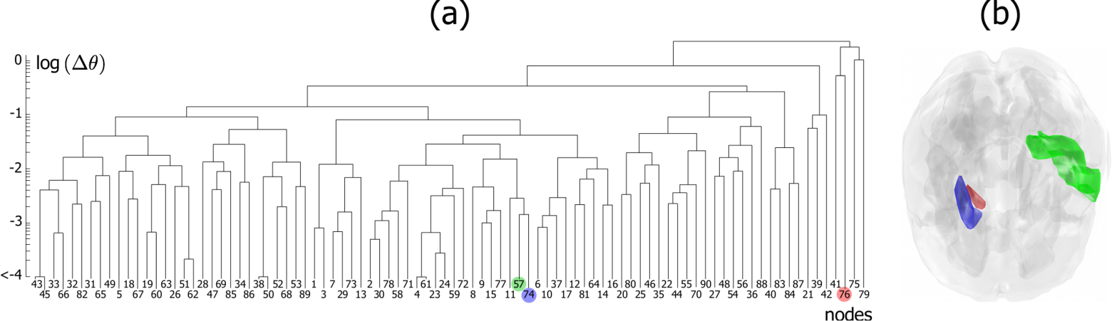
Figure S-1: Hierarchical clustering of phase values obtained from anatomical connectivity in Eq. (1) of the main text. Nodes correspond to the different brain areas. Brain sites with similar and dissimilar phases are colored and superimposed onto an anatomical image (see details in the main text).

Brain data acquisition and pre-processing. – The anatomical connectivity network is based on the connectivity matrix obtained by Diffusion Magnetic Resonance Imaging (DW-MRI) data from 20 healthy participants, as described in DTIdata2008 . The elements of this matrix represent the probabilities of connection between the 90 anatomical regions of interest ($N=90$ nodes in the network) of the Tzourio-Mazoyer brain atlas TzourioMazoyer2002 . These probabilities are proportional to the density of fibers between different areas, so each element of the matrix represents an approximation of the connection strength between the corresponding pair of brain regions.

The functional brain connectivity was extracted from BOLD fMRI resting state recordings obtained as described in valencia2009 . All fMRI data sets (segments of 5 minutes recorded from 15 healthy subjects) were co-registered to the anatomical data set and normalized to the standard MNI (Montreal Neurological Institute) template image, to allow comparisons between subjects. As for DW-MRI data, normalized and corrected functional scans were sub-sampled to the anatomical labeled template of the human brain TzourioMazoyer2002 . Regional time series were estimated for each individual by averaging the fMRI time series over all voxels in each region (data were not spatially smoothed before regional parcellation). To eliminate low frequency noise (e.g. slow scanner drifts) and higher frequency artifacts from cardiac and respiratory oscillations, time-series were digitally filtered with a finite impulse response (FIR) filter with zero-phase distortion (bandwidth $0.01-0.1$ Hz) as in valencia2009 .

Functional synchrony. – A functional link between two time series $x_{i}(t)$ and $x_{j}(t)$ (normalized to zero mean and unit variance) was defined by means of the linear cross-correlation coefficient computed as $r_{ij}=\langle x_{i}(t)x_{j}(t)\rangle$, where $\langle\cdot\rangle$ denotes the temporal average. For the sake of simplicity, we only considered here correlations at lag zero. To determine the probability that correlation values are significantly higher than what is expected from independent time series, $r_{ij}(0)$ values (denoted $r_{ij}$) were firstly transformed by the Fisher’s Z transform

$$Z_{ij}=0.5\ln\left(\frac{1+r_{ij}}{1-r_{ij}}\right)$$ (S-3)

Under the hypothesis of independence, $Z_{ij}$ has a normal distribution with expected value 0 and variance $1/(df-3)$, where $df$ is the effective number of degrees of freedom Bartlett1946 ; Bayley1946 ; Jenkins1968 . If the time series consist of independent measurements, $df$ simply equals the sample size, $N$. Nevertheless, autocorrelated time series do not meet the assumption of independence required by the standard significance test, yielding a greater Type I error Bartlett1946 ; Bayley1946 ; Jenkins1968 . In presence of auto-correlated time series $df$ must be corrected by the following approximation:

$$\frac{1}{df}\approx\frac{1}{N}+\frac{2}{N}\sum_{\tau}r_{ii}(\tau)r_{jj}(\tau),$$ (S-4)

where $r_{xx}(\tau)$ is the autocorrelation of signal $x$ at lag $\tau$.

To estimate a threshold for statistically significant correlations, a correction for multiple testing was used. The False Discovery Rate (FDR) method was applied to each matrix of $Z_{ij}$ values FDR . With this approach, the threshold of significance $Z_{\text{th}}$ was set such that the expected fraction of false positives is restricted to $q\leq 0.05$.

Clustering of phase values. – To identify brain areas that could be related by a topological symmetry, we used the anatomical connectivity obtained from the DW-MRI data as the connectivity matrix ($N=90$ nodes) in Eq. (1) of the main text. A standard hierarchical agglomerative clustering algorithm was then used to identify nodes with similar phases GanBook . The resulting dendrogram is depicted in Fig. S-1.

References

- (1) Pikovsky, A., Rosenblum, M. & Kurths, J. Synchronization: a Universal Concept in Nonlinear Sciences (Cambridge University Press, Cambridge, England, 2003).
- (2) S.H. Strogatz, Nature 410, 268 (2001).
- (3) E. Bullmore and O. Sporns, Nature Reviews Neuroscience 10, 186 (2009).
- (4) M. Chavez, M. Valencia, V. Navarro, V. Latora, and J. Martinerie, Phys. Rev. Lett. 104, 118701 (2010)
- (5) P. Tass, Phase Resetting in Medicine and Biology, (Springer, New York, 1999).
- (6) Y. Kuramoto, Lect. Notes in Physics 30, 420 (1975).
- (7) H. Sakaguchi and Y. Kuramoto, Prog. Theor. Phys. Vol. 76, 576 (1986)
- (8) S.H. Strogatz, Physica D 143, 1 (2000).
- (9) J A Acebrón, L L Bonilla, C J Pérez-Vicente, F Ritort, and R Spigler, Rev. Mod. Phys. 77, 137-185 (2005).
- (10) D.J. Watts and S.H. Strogatz, Nature 393, 440 (1998).
- (11) S. Boccaletti, V. Latora, Y. Moreno, M. Chavez and D.-U. Hwang, Phys. Rep. 424, 175 (2006).
- (12) D. A. Wiley, S. H. Strogatz and M. Girvan, Chaos, 16, 015103 (2006).
- (13) A. Arenas, A. Díaz-Guilera, J. Kurths, Y. Moreno and C. Zhou, Phys. Rep. 469, 93 (2008).
- (14) A. Arenas, A. Díaz-Guilera and C.J. Pérez-Vicente, Phys. Rev. Lett. 96, 114102 (2006).
- (15) S. Boccaletti, M. Ivanchenko, V. Latora, A. Pluchino, A. Rapisarda, Phys. Rev. E 75, 045102(R) (2007).
- (16) J. Gómez-Gardeñes, Y. Moreno and A. Arenas, Phys. Rev. Lett. 98, 034101 (2007).
- (17) R. Gutiérrez, A. Amann, S. Assenza, J. Gómez-Gardenes, V. Latora, S. Boccaletti, Phys. Rev. Lett. 107, 234103 (2011)
- (18) L. Prignano and A. Diaz-Guilera, Phys. Rev. E 85, 036112 (2012).
- (19) S. Fortunato, Phys. Rep. 486, 75 (2010).
- (20) J. Tegnér, M. K. S. Yeung, J. Hasty and J. J. Collins, Proc. Natl. Acad. Sci. USA, 100, 5944-5949 (2003).
- (21) F. Varela, J.-P. Lachaux, E. Rodriguez and J. Martinerie, Nat. Rev. Neurosci. 2, 229 (2001).
- (22) R. Smith, S. Guyomarch, T. Mandel, D. Reinhardt, C. Kuhlemeier, P. Prusinkiewicz, Proc. Natl. Acad. Sci. USA, 103, 5, 1301 (2006).
- (23) I. Ruvinsky, J.J. Gibson-Brown, Development 127, 24, 5233 (2000).
- (24) J. E. Rosenthal and G. M. Murphy, Rev.Mod.Phys. 8, 317 (1936).
- (25) A problem is in the complexity class NP if it can be solved in polynomial time by a nondeterministic Turing machine. A problem is said to be NP-complete if it is in NP and it is NP-hard, i.e., at least as hard to solve as any other problem in NP. See Ref. Papadimitriou1994 for an in-depth discussion of complexity classes.
- (26) C.H. Papadimitriou Computational Complexity (Addison Wesley, Reading, MA, 1994).
- (27) E.M. Luks, J. Comput. System Sci. 25, 42 (1982).
- (28) P. Holme, Phys. Rev. E 74, 036107 (2006).
- (29) P. Holme, Journ. of the Korean Phys. Soc. 50, 300 (2007).
- (30) A. Bergner, M. Frasca, G. Sciuto, A. Buscarino, E. J. Ngamga, L. Fortuna, J. Kurths, Phys. Rev. E 85, 026208 (2012).
- (31) H. Aufderheide, L. Rudolf and T. Gross, New J. Phys. 14, 105014 (2012).
- (32) G. Russo and J.-J. E. Slotine, Phys. Rev. E, 84, 041929 (2011).
- (33) I. Fischer, R. Vicente, J. M. Buldú, M. Peil, C. R. Mirasso, M. C. Torrent and J. García-Ojalvo, Phys. Rev. Lett. 97, 123902 (2006).
- (34) R. Vicente, L. L. Gollo, C. R. Mirasso, I. Fischer and G. Pipa, Proc. Natl. Acad. Sci. USA 105, 17157 (2008).
- (35) A. Viriyopase, I. Bojak, M. Zeitler and S. Gielen, Front. Comput. Neurosci. 6, 49 (2012).
- (36) In general, Eqs. (1) do not admit a fully synchronized stationary state, because the system has no solutions except for regular graphs, where .
- (37) Each row and each column of a permutation matrix has exactly one entry equal to one and all others equal to . If is a permutation matrix, the matrix product swaps pairs of rows of , while swaps pairs of columns of .
- (38) D. M. Abrams, S. H. Strogatz, Phys. Rev. Lett. 93, 174102 (2004).
- (39) C. R. Laing, Physica D, 238, 1569 (2009).
- (40) M. Shanahan, Chaos, 20, 013108 (2010).
- (41) E. A. Martens, C. R. Laing and S. H. Strogatz, Phys. Rev. Lett. 104, 044101 (2010).
- (42) Y. Iturria-Medina, et al. Cerebral Cortex 21, 56 (2011).
- (43) S. Strogatz, Nonlinear Dynamics and Chaos: with applications to physics, biology, chemistry and engineering. (Perseus Books Group, 1994).
- (44) Y. Iturria-Medina, et al. Neuroimage 40, 1064 (2008).
- (45) N. Tzourio-Mazoyer, B. Landeau, D. Papathanassiou, F. Crivello, O. Etard, N. Delcroix, B. Mazoyer, and M. Joliot. Neuroimage 15, 273 (2002).
- (46) M. Valencia, M. A. Pastor, M. A. Fernández-Seara, J. Artieda, J. Martinerie, and M. Chavez. Chaos 19, 023119 (2009).
- (47) M. S. Bartlett J. R. Stat. Soc. B 8, 27 (1946).
- (48) G. V. Bayley, and J. M. Hammersley J. R. Stat. Soc. B 8,184 (1946).
- (49) G. M. Jenkins, and D. G. Watts Spectral analysis and its applications. Holden-Day, San Francisco, California, (1968).
- (50) Y. Benjamini, and Y. Yekutieli, Ann. Statist. 29, 1165 (2001).
- (51) G. Gan, C. Ma, and J. Wu Data clustering: Theory, Algorithms, and Applications. ASA-SIAM Series on Statistics and Applied Probability, SIAM, Philadelphia, ASA, Alexandria, VA, (2007).