Drift in Transaction-Level Asset Price Models

Abstract

We study the effect of drift in pure-jump transaction-level models for asset prices in continuous time, driven by point processes. The drift is assumed to arise from a nonzero mean in the efficient shock series. It follows that the drift is proportional to the driving point process itself, i.e. the cumulative number of transactions. This link reveals a mechanism by which properties of intertrade durations (such as heavy tails and long memory) can have a strong impact on properties of average returns, thereby potentially making it extremely difficult to determine long-term growth rates or to reliably detect an equity premium. We focus on a basic univariate model for log price, coupled with general assumptions on the point process that are satisfied by several existing flexible models, allowing for both long memory and heavy tails in durations. Under our pure-jump model, we obtain the limiting distribution for the suitably normalized log price. This limiting distribution need not be Gaussian, and may have either finite variance or infinite variance. We show that the drift can affect not only the limiting distribution for the normalized log price, but also the rate in the corresponding normalization. Therefore, the drift (or equivalently, the properties of durations) affects the rate of convergence of estimators of the growth rate, and can invalidate standard hypothesis tests for that growth rate. As a remedy to these problems, we propose a new ratio statistic which behaves more robustly, and employ subsampling methods to carry out inference for the growth rate. Our analysis also sheds some new light on two longstanding debates as to whether stock returns have long memory or infinite variance.

1 Introduction

In recent years, transaction-level data on financial markets has become increasingly available, and is now often used to make trading decisions in real time. Such data typically consist of the times at which transactions occurred, together with the price at which the transaction was executed, and may include other concomitant variables (”marks”) such as the number of shares traded. Our focus here is on actual transactions rather than quotes, but regardless of which type of event is being considered it is important to recognize that a useful framework for modeling and analyzing such data is that of marked point processes rather than, say, time series in discrete time. Though time series are typically provided for further analysis, such as daily (or high frequency) stock returns, these inevitably involve aggregation and entail a loss of information that may be crucial for trading and perhaps even for risk management and portfolio selection.

The perspective of asset prices as (marked) point processes has a long history in the financial and econometric literature. For example, Scholes and Williams, (1977) allowed for a compound Poisson process. However, such a model is at odds with the stylized fact that time series of financial returns exhibit persistence in volatility. Recent interest in the point process approach to modeling transaction-level data was spurred by the seminal paper of Engle and Russell, (1998), who proposed a model for inter-trade durations. Other work on modeling transaction-level data as point processes and/or constructing duration models includes that of Prigent, (2001), Bowsher, (2007), Billingsley, (1968), Hautsch, (2012), Bacry et al., (2011), Deo et al., (2009), Deo et al., (2010), Hurvich and Wang, (2010), Aue et al., (2014), Shenai, (2012), Chen et al., (2012).

Nevertheless, it must be recognized that time series of asset returns in discrete (say, equally-spaced) time are still in widespread use, and indeed may be the only recorded form of the data that encompasses many decades. Such long historical series are of importance for understanding long-term trends (a prime focus of this paper) and, arguably, for a realistic assessment of risk. So given the ubiquitous nature of the time series data but also keeping in mind the underlying price-generating process that occurred at the level of individual transactions, it is important to make sure that transaction-level models obey the stylized facts, not only for the intertrade durations but also for the lower-frequency time series.

It has been observed empirically that time series of financial returns are weakly autocorrelated (though perhaps not completely uncorrelated), while squared returns or other proxies for volatility show strong autocorrelations that decay very slowly with increasing lag, possibly suggesting long memory (see Andersen et al., (2001)). It is also generally accepted that such time series show asymmetries, such as a correlation between the current return and the next period’s squared return, and this effect (often referred to traditionally as the ”leverage effect”) is addressed for example by the EGARCH model of Nelson, (1991). The average return often differs significantly from zero based on a traditional $t$-test, possibly suggesting a linear trend in the series of log prices. Meanwhile, Deo et al., (2010) found that intertrade durations have long memory (this was also found by Chen et al., (2012)), and they investigated the possibility that the durations have heavy tails.

One more fact that we wish to stress is that in continuous time, realizations of series of transaction-based asset prices are step functions, since the price is constant unless a transaction occurs. Thus, we choose to focus on pure-jump models for the log price (viewed as a time series in continuous time), driven by a point process that counts the cumulative number of transactions. This is equivalent to a marked point process approach where the points correspond to the transaction times and the marks are the transaction-level return shocks, which can have both an efficient component and a microstructure component.

Within this context, we will in this paper investigate the effect of drift (modeled at the transaction level) on the behavior of very-long-horizon returns, or equivalently, on the asymptotic behavior of the log price as time increases. The drift is assumed to arise from a nonzero mean in the efficient shock series. It follows that the drift is proportional to the driving point process itself, i.e. the cumulative number of transactions. This link reveals a mechanism by which properties of intertrade durations (such as heavy tails and long memory) can have a strong impact on properties of average returns, thereby potentially making it extremely difficult to determine long-term growth rates or to reliably detect an equity premium.

We focus on a basic univariate model for log price, coupled with general assumptions on the point process that are satisfied by several existing flexible models, allowing for both long memory and heavy tails in durations. Under our pure-jump model (which can capture all the stylized facts described above), we obtain the limiting distribution for the suitably normalized log price. This limiting distribution need not be Gaussian, and may have either finite variance or infinite variance. The diversity of limiting distributions here may be considered surprising, since our assumptions imply that the return shocks obey an ordinary central limit theorem under aggregation across transactions ($i.e.$ in $transaction$ $time$ but generally not in $calendar$ $time$). We show that the drift can affect not only the limiting distribution for the normalized log price, but also the rate in the corresponding normalization. Therefore, the drift (or equivalently, the properties of durations) affects the rate of convergence of estimators of the growth rate, and can invalidate standard hypothesis tests for that growth rate. Our analysis also sheds some new light on two longstanding debates as to whether stock returns have long memory or infinite variance.

The remainder of this paper is organized as follows. In Section 2, we provide a simple univariate model for the log price, discuss the trend term and present Proposition 2.1 on the limiting behavior of the log price process, as determined by the properties of the point process. In Section 3 we begin a study of statistical inference for the trend, and obtain the behavior of the ordinary $t$-statistic under the null hypothesis. We also propose a ratio statistic which behaves robustly, in that (unlike the $t$-statistic) it converges in distribution under a broad range of conditions. This motivates our discussion in Section 4 of the use of subsampling based on the ratio statistic to conduct statistical inference on the trend. We then present, in Section 5, a series of examples of specific duration and point process models that have been proposed in the literature, including the Autoregressive conditional duration (ACD) model of Engle and Russell, (1998) and the long memory stochastic duration (LMSD) model of Deo et al., (2010). These examples provide for great diversity of the asymptotic distributions of sums of durations and therefore (by Proposition 2.1 below) for the asymptotic distribution of the log price. Simulations are presented in Section 6. There, we consider the size and power for both the $t$-test and the test based on the new ratio statistic under three duration models: $iid$ exponential, ACD and LMSD. The parameters of simulations are calibrated using empirical data. Section 7 provides a data analysis in which we employ the $t$-test and the test based on the new ratio statistic to gauge the strength of the equity premium. Section 8 provides a concluding discussion on how our results may help to reconcile some longstanding debates. Proofs of the mathematical results are provided in Section 9.

2 A Univariate Model for Log Price

We start with a basic univariate pure-jump model for a log price series $y$. Let $N_{1}$, $N_{2}$ be mutually independent point processes on the real line. Points of $N_{1}+N_{2}$ correspond to transactions on the asset and $(N_{1}+N_{2})(t)$ is the number of transactions in $(0,t]$. We set $y(0)=0$ and define, for $t\geq 0$,

$$y(t)=\sum_{k=1}^{N_{1}(t)}(\tilde{e}_{1,k}+\eta_{1,k})+\sum_{k=1}^{N_{2}(t)}(\tilde{e}_{2,k}+\eta_{2,k})$$ (2.1)

where for $i=1,2$,

$$\tilde{e}_{i,k}=\mu_{i}+e_{i,k}$$

and the $\{e_{i,k}\}$, which are independent of $(N_{1},N_{2})$, are i.i.d. with zero mean and finite variance $\sigma_{i}^{2}$. We assume that the microstructure noise sequences $\{\eta_{i,k}\}$ are independent of the efficient shocks $\{e_{1,k}\}$, $\{e_{2,k}\}$, but not necessarily of the counting process $(N_{1},N_{2})$. This allows for a leverage effect. See Aue et al., (2014). Assumption 2.2 below implies that the microstructure noise becomes negligible after aggregation.

We assume that $\mu_{1}$ and $\mu_{2}$ are constants, not both zero. This model with $\mu_{1}=\mu_{2}=0$, $\sigma_{2}^{2}=0$ and $\{\eta_{2,k}\}=0$ was considered in Deo et al., (2009), who showed that it can produce long memory in the realized volatility. We generalize the model here to allow for two driving processes, $N_{1}$ and $N_{2}$. It follows from (2.1) that

$$y(t)=\mu_{1}N_{1}(t)+\mu_{2}N_{2}(t)+\sum_{k=1}^{N_{1}(t)}(e_{1,k}+\eta_{1,k})+\sum_{k=1}^{N_{2}(t)}(e_{2,k}+\eta_{2,k})\;.$$ (2.2)

The quantity $\mu_{1}N_{1}(t)+\mu_{2}N_{2}(t)$ can be viewed as a random drift term in the log price $y(t)$. If, for example, $\mu_{1}>0$ and $\mu_{2}<0$ then we can think of $N_{1}$ and $N_{2}$ as governing the activity of buyers and sellers, respectively. An active period for $N_{1}$ puts upward pressure on the price, while an active period for $N_{2}$ exerts downward pressure. One could envision including other point processes to differentiate, say, between information traders and noise traders, but we find that the model with just $N_{1}$ and $N_{2}$ is quite flexible and able to reproduce the stylized facts.

To simplify the discussion, we assume temporarily that $N_{1}$ and $N_{2}$ are stationary point processes with intensities $\lambda_{1}$ and $\lambda_{2}$. Then the expectation of the drift term is a linear trend, that is, ${\mathbb{E}}[\mu_{1}N_{1}(t)+\mu_{2}N_{2}(t)]=\mu^{*}t$, where

$$\mu^{*}=\lambda_{1}\mu_{1}+\lambda_{2}\mu_{2}\,\,\,.$$

Since we are modeling the log prices $y(t)$ as a pure-jump process the log price is constant when no trading occurs. Unfortunately, the modified version of (2.2) in which the random drift term $\mu_{1}N_{1}(t)+\mu_{2}N_{2}(t)$ is replaced by the deterministic time trend $ct$ (where $c$ is a nonzero constant) would not yield a pure-jump process. Nevertheless, it is quite reasonable from an economic viewpoint to imagine that ${\mathbb{E}}[y(t)]$ is a linear function of $t$, to account for such phenomena as equity premia and inflation. This is indeed the case for Model (2.2) if it is assumed in addition that the microstructure noise terms have zero mean under their Palm distribution (see below), which implies ${\mathbb{E}}[y(t)]=\mu^{*}t$. But in actual realizations of $y(t)$, the trend is only impounded when a transaction occurs, due to the nonzero means in $\{\tilde{e}_{1,k}\}$ and/or $\{\tilde{e}_{2,k}\}$.

We now obtain conditions under which the two summations on the righthand side of (2.2) have mean zero, so that ${\mathbb{E}}[y(t)]=\mu^{*}t$, still under the assumption that $N_{1}$ and $N_{2}$ are stationary. Since the efficient shocks are assumed independent of $N_{1}$ and $N_{2}$ and have mean zero, it follows that ${\mathbb{E}}\left[\sum_{k=1}^{N_{i}(t)}e_{i,k}\right]=0$. However, due to potential leverage-type effects, even if one were to assume that ${\mathbb{E}}[\eta_{i,k}]=0$, this alone would not ensure that ${\mathbb{E}}\left[\sum_{k=1}^{N_{i}(t)}\eta_{i,k}\right]=0$. Therefore, if we want to interpret expectation of the drift term as a linear trend in the log price, we must make the additional assumption that ${\mathbb{E}}\left[\sum_{k=1}^{N_{i}(t)}\eta_{i,k}\right]=0$. As we will show, this assumption is equivalent to assuming that the $E_{i}^{0}[\eta_{i,k}]=0$, where $P_{i}^{0}$ is the Palm probability measure associated with the point process $N_{i}$, and $E_{i}^{0}$ is the expectation under the Palm measure.

We briefly recall here (see Deo et al., (2009) for more details) that in general there is no single measure under which both the durations and the marked point process are stationary. If the durations for a point process $N$ are stationary under a measure $P^{0}$, then we refer to $P^{0}$ as the Palm probability measure. This, if such a measure exists, would be the appropriate measure for assessing properties of durations as a stationary sequence. In such situations, there exists a corresponding measure ${\mathbb{P}}$ under which the point process is stationary. This would be the appropriate distribution for assessing counts (the number of events occurring in equally spaced intervals of time), and also the differences of $y(t)$ in (2.2), as a stationary time series in models that admit stationarity.

If $\{t_{k},z_{k},k\in{\mathbb{Z}}\}$ are the (marked) points of a stationary (under ${\mathbb{P}}$) marked point process $N$ with finite intensity $\lambda$, then, by Baccelli and Brémaud, (2003, Formula 1.2.9), for all $t>0$

$${\mathbb{E}}\left[\sum_{k=1}^{N(t)}z_{k}\right]=\lambda tE^{0}[z_{0}]\;,$$

where $E^{0}$ is the expectation with respect to the Palm probability $P^{0}$. If the marks $\{z_{k}\}$ have zero mean under the Palm measure $P^{0}$, then ${\mathbb{E}}\left[\sum_{k=1}^{N(t)}z_{k}\right]=0$, even if, under ${\mathbb{P}}$, it might happen that ${\mathbb{E}}[z_{0}]=\lambda E^{0}[t_{1}z_{1}]\neq 0$.

It follows that if the microstructure noise sequences $\{\eta_{i,k}\}$ have zero mean under their respective Palm measures $P_{i}^{0}$ then in the model (2.2) under ${\mathbb{P}}$ we have ${\mathbb{E}}[y(t)]=\mu^{*}t$.

There are a variety of reasons why it may be considered unrealistic to assume that the point process $(N_{1},N_{2})$ is stationary. Indeed, it is well-known that the counts of financial transactions can show intraday seasonality (see, e.g., Engle and Russell, (1998), Deo et al., (2010)), and the transaction counts will be guaranteed to be zero when the market is not open for trading. Furthermore, regime changes are widely understood to be an important feature of economic processes. We will consider a time deformation mechanism below which allows for such effects. In the absence of stationarity we are no longer able to compute ${\mathbb{E}}[y(t)]$ in (2.2), but we can still interpret $\mu^{*}$ as a long term trend, i.e. $y(t)/t{\ \stackrel{{\scriptstyle\mathbb{P}}}{{\to}}}\ \mu^{*}$, under the assumptions below. These assumptions are stronger than needed for this purpose but will be used later to derive limiting distributions for suitably rescaled versions of $y$.

In the sequel, we will consider a single probability measure ${\mathbb{P}}$, without any requirement that $(N_{1},N_{2})$ be stationary under ${\mathbb{P}}$, unless specified otherwise. Convergence in ${\mathbb{P}}$-probability will be denoted by ${\ \stackrel{{\scriptstyle\mathbb{P}}}{{\to}}}\$, convergence in distribution under ${\mathbb{P}}$ of sequences of random variables will be denoted by ${\to}$ and convergence of finite dimensional distributions of a sequence of stochastic processes will be denoted by $\ \stackrel{{\scriptstyle fi.di.}}{{\longrightarrow}}\$.

Assumption 2.1.

The point processes $N_{1}$ and $N_{2}$ are mutually independent and there exists $\gamma\geq 1/2$ such that

$$\{n^{-\gamma}(N_{i}(nt)-\lambda_{i}nt),t\geq 0\}\ \stackrel{{\scriptstyle fi.di.}}{{\longrightarrow}}\ A_{i}$$ (2.3)

for $i=1,2$, as $n\rightarrow\infty$ where $A_{i}$ are stochastic processes, at least one of which is nonzero.

We will give examples of point processes satisfying Assumption 2.1 in Section 5. As will be seen, the limiting processes $A_{i}$ can be Gaussian or have infinite variance, can have independent or dependent increments, and $\gamma$ can take any value in $[1/2,1)$. However, whatever $A$ and $\gamma$, a consequence of the convergence (2.3) is that $N_{i}(t)/t{\ \stackrel{{\scriptstyle\mathbb{P}}}{{\to}}}\ \lambda_{i}$ and $t^{-1/2}\sum_{k=1}^{N_{i}(t)}e_{i,k}$ converges weakly to a Brownian motion.

Two distinct modeling approaches seem natural. One is to model the point process directly as in Bacry et al., (2011) who use Hawkes processes or Delattre et al., (2013) who use Cox processes. Another approach consists of modeling the durations. This was done by Engle and Russell, (1998) who defined the ACD model and Deo et al., (2010) who defined the LMSD model. These two approaches are equivalent with respect to Assumption 2.1, since (2.3) with limit process $A$ holds for a point process $N$ with intensity $\lambda$ and duration sequence $\{\tau_{k}\}$ if and only if

$$n^{-\gamma}\sum_{k=1}^{[n\cdot]}(\tau_{k}-\lambda^{-1})\ \stackrel{{\scriptstyle fi.di.}}{{\longrightarrow}}\ -\lambda^{-(1+\gamma)}A\;,$$ (2.4)

where convergence holds in the sense of finite dimensional distributions. See Whitt, (2002, Theorem 7.3.1).

Assumption 2.2.

The sequence of processes $n^{-1/2}\sum_{k=1}^{[n\cdot]}\eta_{i,k}$ converges in probability uniformly on compact sets to 0.

Assumptions 2.1 and 2.2 imply that $t^{-1/2}\sum_{k=1}^{N_{i}(t)}(e_{i,k}+\eta_{i,k})$ converges weakly to a Brownian motion and so the microstructure terms are asymptotically negligible.

The following proposition, which follows easily from Assumptions 2.1 and 2.2, gives the limiting distribution for suitably rescaled versions of the log price process $y$. Recall that Assumption 2.1 implies that $N_{i}(t)/t{\ \stackrel{{\scriptstyle\mathbb{P}}}{{\to}}}\ \lambda_{i}$. Let $\mu^{*}=\lambda_{1}\mu_{1}+\lambda_{2}\mu_{2}$.

Proposition 2.1.

Let Assumptions 2.1 and 2.2 hold. Then $y(t)/t{\ \stackrel{{\scriptstyle\mathbb{P}}}{{\to}}}\ \mu^{*}$. Moreover, as $n\rightarrow\infty$,

$$\{n^{-\gamma}(y(nt)-\mu^{*}nt),t\geq 0\}\ \stackrel{{\scriptstyle fi.di.}}{{\longrightarrow}}\ \mu_{1}A_{1}+\mu_{2}A_{2}\;,$$ (2.5)

if $\gamma>1/2$ and

$$\{n^{-1/2}(y(nt)-\mu^{*}nt),t\geq 0\}\ \stackrel{{\scriptstyle fi.di.}}{{\longrightarrow}}\ \mu_{1}A_{1}+\mu_{2}A_{2}+\sigma B$$ (2.6)

if $\gamma=1/2$ or if $\mu_{1}=\mu_{2}=0$, where $B$ is a standard Brownian motion independent of $A_{i}$ and $\sigma$ is a positive constant.

Next, we discuss the use of time deformation. This discussion is taken from Aue et al., (2014). Let $f$ be a deterministic or random function such that $f$ is nondecreasing and has càdlàg paths with probability one. Let $\tilde{N}$ be a point process and define

$$N(t)=\tilde{N}(f(t))\;.$$

We do not require that $\tilde{N}$ be stationary, but one useful application of time deformation is to start with a stationary process $\tilde{N}$ and then deform it as above to obtain a nonstationary process $N$. If the function $f$ is random, we assume moreover that it is independent of $\tilde{N}$. The use of the time-varying intensity function $f$ may render the counting process $N$ nonstationary even if $\tilde{N}$ is a stationary point process. Since it is possible that $f$ has (upward) jumps, the point process $N$ may also not be simple even though $\tilde{N}$ is simple. We now show, however, that if $\tilde{N}$ satisfies Assumption 2.1, then so does the time-deformed $N$ under some restrictions on $f$.

Lemma 2.1.

Assume that $f$ is a nondecreasing (random) function such that $t^{-1}f(t){\ \stackrel{{\scriptstyle\mathbb{P}}}{{\to}}}\ \delta\in(0,\infty)$ and

$$\sup_{t\geq 0}|f(t)-f(t^{-})|\leq C$$

with probability one, where $C\in(0,\infty)$ is a deterministic constant. Let $\tilde{N}$ be a point process such that Assumption 2.1 holds for some $\tilde{\lambda}\in(0,\infty)$ and $\gamma>0$. Let $N$ be the counting process defined by $N(\cdot)=\tilde{N}(f(\cdot))$. Then Assumption 2.1 holds for $N$ with $\lambda=\tilde{\lambda}\delta$.

The function $f$ is used to speed up or slow down the trading clock. To incorporate dynamic intraday seasonality in volatility, the same time deformation can be used in each trading period (of length, say, $T$), assuming that $f(t)$ has a periodic derivative (with period $T$ and with probability one), for example, $f(t)=t+.5\sin(2\pi t/T)$. Fixed nontrading intervals, say, $t\in[T_{1},T_{2})$, could be accommodated by taking $f(t)=f(T_{1})$ for $t\in[T_{1},T_{2})$ so that $f(t)$ remains constant for $t$ in this interval, and then taking $f(T_{2})>f(T_{1})$ so that $f(t)$ jumps upward when trading resumes at time $T_{2}$. The jump allows for the possibility of one or more transactions at time $T_{2}$, potentially reflecting information from other markets or assets that did trade in the period $[T_{1},T_{2})$. Since it is possible that $f$ has (upward) jumps, $N$ may not be simple even though $\tilde{N}$ is simple.

3 Statistical inference for the trend

For integer $k$, (assuming a time-spacing of 1 without loss of generality) we define the calendar-time returns as $r_{k}=y(k)-y(k-1)$ and the average return over a time period that extends from time $0$ to time $n$ as $\bar{r}_{n}=n^{-1}y(n)=n^{-1}\sum_{k=1}^{n}r_{k}$. We can think of $n$ as the length of the time interval spanned by the observations, or (since we have assumed a time-spacing of 1) as the sample size, $i.e.$, the number of observed returns. It follows from Proposition 2.1 that if $\gamma>1/2$, $\bar{r}_{n}-\mu^{*}$ will not be $O_{p}(n^{-1/2})$, making it difficult to accurately estimate growth rates based on the data set $\{r_{k}\}_{k=1}^{n}$.

We recall that model (2.2) under stationarity of $N_{1}$ and $N_{2}$ implies that ${\mathbb{E}}[y(n)]=\mu^{*}n$, so that the growth rate per unit time is $\mu^{*}$, but that under the more general assumptions 2.1 and 2.2 $\mu^{*}$ may still be viewed as a long-term growth rate, since $y(n)/n{\ \stackrel{{\scriptstyle\mathbb{P}}}{{\to}}}\ \mu^{*}$.

We consider the problem of statistical inference for $\mu^{*}$. We focus on testing a null hypothesis of the form $H_{0}:\mu^{*}=\mu_{0}^{*}$ based on $\bar{r}_{n}$.

3.1 The $t$ statistic

The corresponding $t$-statistic for testing $H_{0}$ is

$$t_{n}=n^{1/2}(\bar{r}_{n}-\mu_{0}^{*})/s_{n},$$

where

$$s_{n}^{2}=(n-1)^{-1}\sum_{j=1}^{n}(r_{j}-\bar{r}_{n})^{2}.$$

The sample variance $s_{n}^{2}$ consistently estimates a positive constant, under suitable moments assumptions.

Lemma 3.1.

Under Assumptions 2.1 and 2.2, if $N_{1}$ and $N_{2}$ are stationary and ergodic and

$${\mathbb{E}}\left[\left(\sum_{k=1}^{N_{i}(1)}(\mu_{i}+e_{i,k}+\eta_{i,k})\right)^{2}\right]<\infty\;,$$ (3.1)

there exists $\varsigma>0$ such that $s_{n}^{2}{\ \stackrel{{\scriptstyle\mathbb{P}}}{{\to}}}\ \varsigma^{2}$.

Since the efficient shocks have zero mean and finite variance and are independent of the point processes, a sufficient condition for (3.1) to hold is ${\mathbb{E}}[N_{i}^{2}(1)]<\infty$ and

$${\mathbb{E}}\left[\left(\sum_{k=1}^{N_{i}(1)}\eta_{i,k}\right)^{2}\right]<\infty\;.$$

If $\gamma>1/2$ and $\mu_{1}$ and $\mu_{2}$ not both zero, it follows from the convergence (2.5) and Lemma 3.1 that if the null hypothesis is true, then $t_{n}=O_{p}(n^{\gamma-1/2})$ and the $t$-statistic diverges under the null hypothesis. Examples where this scenario would occur include durations generated by an LMSD model with long memory and an exponential volatility function. This scenario therefore is consistent with the empirical properties of durations found in Deo et al., (2010).

If $\gamma=1/2$ or if $\mu_{1}=\mu_{2}=0$, then $t_{n}{\to}A(1)/\varsigma$ where $A$ is the limiting process in (2.6), i.e. the $t$-statistic converges to a non degenerate distribution, but the $t$-test will not be asymptotically correctly sized, except under very specific circumstances. First the limits $A_{1},A_{2}$ must have normal distributions. This would happen, for example, if the durations are i.i.d. with finite variance (as would be the case for the Poisson process), or if the durations obey an ACD model with finite variance. Then it would also be necessary that $\lim_{t\rightarrow\infty}t^{-1/2}{\mathrm{var}}[N_{i}(t)]={\mathrm{var}}[N_{i}(1)]$, which would hold for instance if $N$ is a Poisson process but would fail if counts are autocorrelated as would typically be the case.

3.2 A ratio statistic

Instead of using the $t$-statistic which could be degenerate, unless the parameter $\gamma$ is equal to 1/2, we propose to use another self-normalized statistic which will always have a non degenerate distribution and does not need additional assumptions. Define $\bar{r}(n)=\bar{r}_{n}$ and

$$T_{n}=\frac{\bar{r}(n)-\mu_{0}^{*}}{|\bar{r}(n)-\bar{r}(n/2)|}\;.$$ (3.2)

Theorem 3.1.

If Assumptions 2.1 and 2.2 hold, then under the null hypothesis $\mu^{*}=\mu_{0}^{*}$,

$$T_{n}{\to}\frac{A(1)}{|A(1)-2A(1/2)|}\;,$$ (3.3)

where $A$ denotes the limiting process in (2.5) if $\gamma>1/2$ and $\mu_{1}$ and $\mu_{2}$ not both zero, or (2.6) if $\gamma=1/2$. If $\mu^{*}>\mu_{0}^{*}$, then $T_{n}{\ \stackrel{{\scriptstyle\mathbb{P}}}{{\to}}}\ +\infty$ and if $\mu^{*}<\mu_{0}^{*}$, then $T_{n}{\ \stackrel{{\scriptstyle\mathbb{P}}}{{\to}}}\ -\infty$.

4 Subsampling

Let $D_{n}(x)$ be the cumulative distribution of $T_{n}$, that is, $D_{n}(x)=\mathbb{P}(T_{n}\leq x)$. Let $D$ denote the corresponding limiting distribution,

$$D=\frac{A(1)}{|A(1)-2A(1/2)|}$$

To perform a hypothesis test on $\mu^{*}$ based on $T_{n}$, we need to approximate $D_{n}(x)$. Since the limiting distribution D will be unknown in practice, we will approximate $D_{n}(x)$ non-parametrically via subsampling.

In subsampling we split the sample into overlapping blocks of size $b$, where $b$ depends on $n$ ($b\rightarrow\infty,b/n\rightarrow 0$), given by $\{r_{t},r_{t+1},...,r_{t+b-1}\}$, $t=1,2,...,n-b+1$, and calculate the self-normalized statistic upon each block, treating each block as if it were a full sample. Moreover, the parameter $\mu_{0}^{*}$ is replaced by its full-sample estimate $\bar{r}(n)$. This leads to $n-b+1$ subsampling statistics

$$T_{n,b,t}=\frac{\bar{r}(n,b,t)-\bar{r}(n)}{|\bar{r}(n,b,t)-\bar{r}(n,b/2,t)|},$$

$$t=1,2,...,n-b+1;\;b\;is\;even,$$

where

$$\bar{r}(n) =\frac{1}{n}\sum\limits_{k=1}^{n}r_{k},$$

$$\bar{r}(n,b,t) =\frac{1}{b}\sum\limits_{k=t}^{t+b-1}r_{k},$$

$$\bar{r}(n,b/2,t) =\frac{2}{b}\sum\limits_{k=t}^{t+b/2-1}r_{k}.$$

The cumulative distribution $D_{n}(x)$ is then approximated by the empirical cdf of these statistics

$$\hat{D}_{n,b}(x)=\frac{1}{n-b+1}\sum\limits_{t=1}^{n-b+1}1_{\{T_{n,b,t}\leq x\}}\;.$$

Let $c_{n,b}(\alpha)$ denote the $\alpha$ quantile of the subsampling distribution, $\hat{D}_{n,b}(x)$,

$$c_{n,b}(\alpha)=\inf\{x:\hat{D}_{n,b}(x)\geq\alpha\}.$$

Then the rejection region for the subsmapling test based on $T_{n}$ in the two-sided case

$$H_{0}:\mu^{*}=\mu_{0}^{*}$$

$$H_{1}:\mu^{*}\neq\mu_{0}^{*}$$

is

$$\{T_{n}<c_{n,b}(\alpha/2)\;or\;T_{n}>c_{n,b}(1-\alpha/2)\}\;.$$

To show that the resulting subsampling test based on $T_{n}$ has asymptotically the nominal size ($\alpha$), we use Theorem 4 of Appendix B of Jach et al., (2012). In order to apply this theorem, we must establish the $\theta$-weak dependence of the time series $\{r_{k}\}$ (see Doukhan and Louhichi, (1999); Bardet et al., (2008)). We will establish this $\theta$-weak dependence for one of the processes we consider in Section 5 (see Proposition 5.1). We say that the subsampling estimator $\hat{D}_{n,b}(x)$ is consistent if $|\hat{D}_{n,b}(x)-D_{n}(x)|{\ \stackrel{{\scriptstyle\mathbb{P}}}{{\to}}}\ 0$ as $n\rightarrow\infty$ for all $x$. The following theorem can be proved based on Theorem 4, Appendix A of Jach et al., (2012) and its proof, as well as the discussion on page 941 of McElroy and Jach, (2012).

Theorem 4.1.

Assume that the time series of calendar-time returns $\{r_{n},n\geq 1\}$ is strictly stationary and $\theta$-weak dependent with rate $\theta_{h}=O(h^{-a})$ up to slowly varying functions. Assume also that the cumulative distribution function of

$$\frac{A(1)}{|A(1)-2A(1/2)|}$$

in Theorem 3.1 is continuous. Then

1. for $a\geq 1/2$, the subsampling estimator is consistent and the resulting test based on $T_{n}$ is asymptotically correctly sized and has power tending to 1 under the alternative hypothesis for any choice of the block size $b$ such that $b\rightarrow\infty$ and $b/n\rightarrow 0$;

2. for $a<1/2$, the subsampling estimator is consistent and the resulting test based on $T_{n}$ is asymptotically correctly sized and has power tending to 1 under the alternative hypothesis if $b\rightarrow\infty$ and $b=O(n^{\zeta})$ (up to slowly varying functions) for some $0<\zeta<2a$.

The theorem gives little guidance as to the choice of the block size $b$ in practice. In the simulations of Section 6 , we will consider a variety of choices of the block size.

5 Examples

In this section we give several examples of point processes which satisfy Assumption 2.1 with $\gamma>1/2$.

5.1 ACD durations

Assume that under the durations form an ACD(1,1) process, defined by

$$\tau_{k} =\psi_{k}\epsilon_{k},\qquad\psi_{k}=\omega+\alpha\tau_{k-1}+\beta\psi_{k-1},\qquad k\in{\mathbb{Z}},$$ (5.1)

where $\omega>0$ and $\alpha,\beta\geq 0$, $\{\epsilon_{k}\}_{k=-\infty}^{\infty}$ is an i.i.d. sequence with $\epsilon_{k}\geq 0$ and ${\mathbb{E}}[\epsilon_{0}]=1$. If $\alpha+\beta<1$, there exists a strictly stationary solution determined by $\tau_{k}=\omega\epsilon_{k}\sum_{j=1}^{\infty}\prod_{i=1}^{j-1}(\alpha\epsilon_{k-i}+\beta)$, with finite mean ${\mathbb{E}}[\tau_{0}]=\omega/(1-\alpha-\beta)$. The tail index $\kappa$ of a ACD(1,1) process is the solution of the equation

$${\mathbb{E}}[(\alpha\epsilon_{0}+\beta)^{\kappa}]=1\;.$$

Moreover the stationary distribution satisfies ${\mathbb{P}}(\tau_{1}>x)\sim cx^{-\kappa}$ for some positive constant $c$. See e.g. Basrak et al., (2002).

• If $1<\kappa<2$, and if $\epsilon_{0}$ has a positive density on $[0,\infty)$, then the finite dimensional distributions of $n^{-1/\kappa}\sum_{k=1}^{[nt]}(\tau_{k}-{\mathbb{E}}[\tau_{0}])$ converges to a totally skewed to the right $\kappa$-stable law. Cf. Bartkiewicz et al., (2011, Proposition 5).

• A necessary and sufficient condition for ${\mathbb{E}}[\tau_{0}^{2}]<\infty$ is ${\mathbb{E}}[(\alpha\epsilon_{0}+\beta)^{2}]=\alpha^{2}{\mathbb{E}}[\epsilon_{0}^{2}]+2\alpha\beta+\beta^{2}<1$. Cf. Giraitis and Surgailis, (2002, Example 3.3). Under this condition, it also holds that $\sum_{k=1}^{\infty}{\mathrm{cov}}(\tau_{0},\tau_{k})<\infty$. Since the ACD process is associated, the summability of the covariance function implies the functional central limit theorem for the partial sum process. See Newman and Wright, (1981). Thus the convergence (2.3) holds with $\gamma=1/2$ and the limit process is the Brownian motion.

This implies that the convergence (2.3) holds with $\gamma=1/\kappa$ and the limit process is a Lévy-stable process if $\kappa<2$ and with $\gamma=1/2$ and the limit process is the Brownian motion if ${\mathbb{E}}[(\alpha\epsilon_{0}+\beta)^{2}]<1$.

5.2 LMSD durations

Assume that the durations form an LMSD process, defined by $\tau_{k}=\epsilon_{k}\sigma(Y_{k})$, where $\{\epsilon_{k},k\in{\mathbb{Z}}\}$ is an i.i.d. sequence of almost surely positive random variables with finite mean and $\{Y_{k},k\in{\mathbb{Z}}\}$ is a stationary standard Gaussian process, independent of $\{\epsilon_{k}\}$ and $\sigma$ is a positive function. As in Deo et al., (2010), for simplicity we will assume that $\sigma(x)={\mathrm{e}}^{x}$.

Assume that the covariance of the Gaussian process $\{Y_{k}\}$ is such that

$$\rho_{n}={\mathrm{cov}}(Y_{0},Y_{n})\sim cn^{2H-2}\;,$$

where $H\in(1/2,1)$ and $c>0$. Denote $\lambda^{-1}={\mathbb{E}}[\epsilon_{0}]{\mathbb{E}}[\exp(Y_{0})]$. Then we have the following possibilities.

• If ${\mathbb{E}}[\epsilon_{k}^{2}]<\infty$, then

  $$n^{-H}\sum_{k=1}^{[n\cdot]}(\tau_{k}-\lambda^{-1})\ \Rightarrow\ \varsigma B_{H}\;,$$

  where $\varsigma$ is a nonzero constant and $B_{H}$ is the standard fractional Brownian motion.

• If ${\mathbb{P}}(\epsilon_{1}>x)\sim cx^{-\alpha}$ as $x\to\infty$ with $\alpha\in(1,2)$, then ${\mathbb{E}}[\epsilon_{k}^{2}]=\infty$ and the following dichotomy is proved in Kulik and Soulier, (2012).

  • If $H>1-1/\alpha$, then

    $$n^{-H}\sum_{k=1}^{[n\cdot]}(\tau_{k}-\lambda^{-1})\ \Rightarrow\ \varsigma B_{H}\;.$$

  • If $H<1-1/\alpha$, then

    $$n^{-1/\alpha}\sum_{k=1}^{[n\cdot]}(\tau_{k}-\lambda^{-1})\ \Rightarrow\ L_{\alpha}\;,$$

    where $L_{\alpha}$ is a totally skewed to the right $\alpha$-stable Lévy process.

We thus see that (2.3) may hold with $\gamma=H$ in the first case and $\gamma=1/\alpha$ with a stable non Gaussian limit in the latter case.

5.3 Superposition of independent point processes

This is an example showing that the limiting distribution of a centered and normalized counting process $N$ may be stable (hence heavy tailed) even though its durations $\tau_{k}$ are light tailed. Let $M_{1}$ be a Poisson process with intensity $\lambda$ and durations $\{\tau_{k}^{(1)}\}$ and $M_{2}$ be a renewal process, independent of $M_{1}$, with i.i.d. durations $\{\tau_{k}^{(2)}\}$ in the normal domain of attraction of a stable law, i.e.

$$n^{-1/\alpha}\sum\limits_{k=1}^{[nt]}(\tau_{k}^{(2)}-\lambda_{2}^{-1})\ \stackrel{{\scriptstyle fi.di.}}{{\longrightarrow}}\ \mathbf{S}(t)\;,$$

where $\alpha\in(1,2)$, $\lambda_{2}^{-1}={\mathbb{E}}[\tau_{1}^{(2)}]$ and $\mathbf{S}$ is a totally skewed to the right $\alpha$-stable Lévy process. By the CLT equivalence, this implies that

$$n^{-1/\alpha}(M_{2}(nt)-\lambda_{2}nt)\ \stackrel{{\scriptstyle fi.di.}}{{\longrightarrow}}\ \mathbf{S}(t)\;.$$

Since the durations of the Poisson process are i.i.d. with finite variance, $n^{-1/2}(M_{1}(nt)-\lambda_{1}nt)$ converges weakly to a Brownian motion. Thus defining the superposition $N$ of these two point processes by

$$N=M_{1}+M_{2}\;,$$

we obtain that

$$n^{-1/\alpha}(N(nt)-\lambda nt)\ \stackrel{{\scriptstyle fi.di.}}{{\longrightarrow}}\ -\lambda_{2}^{1+1/\alpha}\mathbf{S}(t)\;,$$

with $\lambda=\lambda_{1}+\lambda_{2}$.

Let $\{\tau_{k}\}$ be the duration sequence of the point process $N$. We now show that the durations are light tailed under the Palm measure $P^{0}$ under which they form a stationary sequence. It follows from the formula (1.4.5) and example 1.4.1 in Baccelli and Brémaud, (2003) that

$$P^{0}(\tau_{1}>x) =\lambda^{-1}{\mathrm{e}}^{-\lambda_{1}x}\left\{\lambda_{1}\bar{F}_{2}(x)+\lambda_{2}\bar{H}_{2}(x)\right\}\;,$$

where $F_{2}$ is the distribution function of $\tau_{1}^{(2)}$ and $H_{2}$ is the corresponding delay distribution defined by $H_{2}(x)=\lambda\int_{0}^{x}\bar{F}_{2}(t)\,{\mathrm{d}}t$. This yields that $P^{0}(\tau_{1}>x)\leq{\mathrm{e}}^{-\lambda_{1}x}$, i.e. the durations of the superposition process are light tailed.

5.4 Cox processes

Consider now a Cox process $N$ driven by a stationary random measure $\xi$, which means that conditionally on $\xi$, $N$ is a Poisson point process with mean measure $\xi$. Then, denoting $\xi(t)=\xi([0,t])$, we have ${\mathbb{E}}[N(t)]={\mathbb{E}}[\xi(t)]=\lambda t$ with $\lambda={\mathbb{E}}[\xi(1)]$ and

$${\mathrm{var}}(N(t))={\mathbb{E}}[\xi(t)]+{\mathrm{var}}(\xi(t))=\lambda t+{\mathrm{var}}(\xi(t))\;.$$

If the stationary random measure $\xi$ has long memory with Hurst index $H>1/2$ then so has $N$. We give examples.

1. Consider the random measure $\xi$ with density ${\mathrm{e}}^{\sigma Z_{H}(s)}$ with respect to Lebesgue’s measure on ${\mathbb{R}}$, where $\sigma>0$ and $Z_{H}$ is a standard fractional Gaussian noise with Hurst index $H\in(1/2,1)$, i.e. a Gaussian stationary process with covariance function $\rho_{H}(t)=\frac{1}{2}\{|t-1|^{2H}-2|t|^{2H}+|t+1|^{2H}\}$. This means that for any Borel set $A$, $\xi(A)=\int_{A}{\mathrm{e}}^{Z_{H}(s)}\,{\mathrm{d}}s$, and in particular $\xi(t)=\int_{0}^{t}{\mathrm{e}}^{Z_{H}(s)}\,{\mathrm{d}}s$. Then, by stationarity,

   $$\lambda={\mathbb{E}}\left[\int_{0}^{1}{\mathrm{e}}^{\sigma Z_{H}(s)}\,{\mathrm{d}}s\right]={\mathbb{E}}\left[{\mathrm{e}}^{\sigma Z_{H}(0)}\right]={\mathrm{e}}^{-\sigma^{2}/2}\;.$$

   Since the function $x\to{\mathrm{e}}^{x}$ has Hermite rank 1, it holds that ${\mathrm{cov}}({\mathrm{e}}^{Z_{H}(0)},{\mathrm{e}}^{Z_{H}(t)})\sim c\rho_{H}(t)$ and ${\mathrm{var}}(\xi(t))\sim C^{2}t^{2H}$ where $c$ and $C$ are positive constants, and $n^{-H}\{\int_{0}^{nt}{\mathrm{e}}^{Z_{H}(s)}\,{\mathrm{d}}s-\lambda nt\}\ \stackrel{{\scriptstyle fi.di.}}{{\longrightarrow}}\ CB_{H}(t)$. See Arcones, (1994) and Dobrushin and Major, (1979) for details about Hermite ranks, covariance inequality and convergence in distribution of integrals of functions of Gaussian processes. Applying Lemma 9.1, we obtain the convergence

   $$n^{-H}\{N(nt)-\lambda nt\}\ \stackrel{{\scriptstyle fi.di.}}{{\longrightarrow}}\ CB_{H}(t)\;.$$

2. Consider the case where the stochastic intensity can be expressed as $\xi(t)=\int_{0}^{t}W(s)\,{\mathrm{d}}s$, where $W(t)$ is an alternating renewal or ON-OFF process (cf.Heath et al., (1998), Daley, (2010)), defined by $W(t)=1$ if $T_{2n}\leq t<T_{2n+1}$ and $T_{2n+1}\leq t<T_{2n+2}$, where $T_{2n}=\sum_{i=0}^{n}X_{i}+Y_{i}$ and $T_{2n}=\sum_{i=0}^{n}X_{i}+Y_{i}+X_{n+1}$, $\{X_{i},i\geq 1\}$ and $\{Y_{i},i\geq 1\}$ are two independent i.i.d. sequences of positive random variables with finite mean (the ON and OFF periods) and $X_{0}$ and $Y_{0}$ are mutually independent and independent of the other random variables, whose distributions are the delay distributions which make the renewal processes stationary. If the ON distribution is regularly varying at infinity with tail index $\alpha\in(1,2)$ i.e. ${\mathbb{P}}(X_{1}>x)\sim cx^{-\alpha}$ as $x\to\infty$ (which implies infinite variance) and if ${\mathbb{E}}[Y_{i}^{\alpha+\epsilon}]<\infty$ for some $\epsilon>0$, then ${\mathrm{var}}(\xi(t))\sim Ct^{2H}$ with $H=(3-\alpha)/2$. Moreover, $n^{-1/\alpha}\{\xi(nt)-\lambda nt\}\ \stackrel{{\scriptstyle fi.di.}}{{\longrightarrow}}\ \Lambda(t)$, where $\Lambda$ is a totally skewed to the right $\alpha$-stable process. Applying Lemma 9.1, we obtain the convergence

   $$n^{-1/\alpha}\{N(nt)-\lambda nt\}\ \stackrel{{\scriptstyle fi.di.}}{{\longrightarrow}}\ \Lambda(t)\;.$$

Proposition 5.1.

Consider the returns $\{r_{n}\}_{n\in\mathbb{N}^{*}}$ driven by a Cox process of case (i), then the conclusion of Theorem 4.1 holds with $a=2-2H$.

Proof of Proposition 5.1.

First note that the causal Gaussian process $Z_{H}(s)$ is $\theta$-weak dependent with rate $\theta_{h}=L(h)h^{2H-2}$ by Bardet et al., (2008), where $L(h)$ is a slowly varying function. Then by the Proposition 1 of Jach et al., (2012), the stationary process $w(s)=e^{\sigma Z_{H}(s)}$ is $\theta$-weak dependent with the same rate. Using Lemma 9.2, we have that the returns $\{r_{n}\}_{n\in\mathbb{N}^{*}}$ are $\theta$-weak dependent with the same rate $\theta_{h}=O(h^{2H-2})$. The cumulative distribution function of

$$\frac{\Lambda(1)}{|\Lambda(1)-2\Lambda(1/2)|}$$

is continuous, where $\Lambda(1)$ and $\Lambda(1/2)$ have totally skewed to the right $\alpha$-stable distributions. Finally, by applying Theorem 4.1 with $a=2-2H$, the result is proved. ∎

6 Simulation

We study the performance of the ordinary $t$-test and the subsampling-based $T$ test of

$$H_{0}:\mu^{*}=0$$ (6.1)

$$H_{1}:\mu^{*}>0$$ (6.2)

We consider exponential, ACD(1,1), and LMSD durations. In each case, we simulate two mutually independent durations process $\{\tau_{k}^{(i)}\}$ for $i=1,2$, and then obtain the corresponding counting processes $\{N_{i}(t)\}$. Next, we generate mutually independent disturbance series $\{\tilde{e}_{k}^{(1)}\}$ and $\{\tilde{e}_{k}^{(2)}\}$ that are i.i.d. Gaussian with means $\mu_{1}>0$, $\mu_{2}<0$, $\mu_{1}+\mu_{2}>0$, and with finite variances $\sigma_{i}^{2}$. For simplicity, we assume all parameters other than $\mu_{i}$ for the two processes to be the same. For the exponential and EACD(1,1) models, we only include the efficient shocks in simulations, and for the LMSD, we also include microstructure shocks, $\{\eta_{k}^{(i)}\}$, that induce a leverage effect. We then construct the log-price series $\{y(k)\}_{k=1}^{n}$ and return series $\{r_{k}\}_{k=1}^{n}$ from (2.2) and $r_{k}=y(k)-y(k-1)$ with $y(0)=0$. We calculate $t_{n}$ and $T_{n}$ based on return series and apply subsampling to obtain the empirical quantiles of $T_{n}$ and thereby carry out the hypothesis test.

We do a preliminary study on the sensitivity of our results to the choice of the block size $b$. These results show insensitivity except for the largest values of $b$.

The simulation results show that in all three models, the $T$ test is generally correctly sized. But in the exponential case where the usual $t$ test is also correctly sized, the power of $T$ is lower than that of the $t$ test. To improve the power, we modify the test statistic defined in (3.2) as

$$T_{n,2}=\frac{\bar{r}(n,n,1)-\mu_{0}^{*}}{|\bar{r}(n,n/2,1)-\bar{r}(n,n/4,1)|+|\bar{r}(n,n/2,n/2+1)-\bar{r}(n,n/4,n/2+1)|}\;,$$ (6.3)

where $\bar{r}(n,b,t)=\frac{1}{b}\sum\limits_{k=t}^{t+b-1}r_{k}$. In the remainder of this section, we will use $T_{1}$ to denote (3.2), $T_{2}$ to denote (6.3), and “$T$ test” to denote a test based on either $T_{1}$ or $T_{2}$.

6.1 Exponential durations

We generate $\{\tau_{k}^{(1)}\}$, $\{\tau_{k}^{(2)}\}$ from exponential distributions $\tau_{k}^{(i)}\ \stackrel{{\scriptstyle i.i.d.}}{{\sim}}\ Exp(\lambda_{i})$, which result in $N_{1}(t)$ and $N_{2}(t)$ being Poisson processes. Since the returns are i.i.d, the $t$-test is correctly sized. Our goal is to study the size of the $T$ test and to compare the power of the $T$ to that of the $t$ test.

6.1.1 Parameter calibration

We consider a total of 30 configurations of parameters and sample size, 15 for evaluating size (Table 2), and 15 for evaluating power (Table 3). The model has six parameters ($\lambda_{1}$, $\lambda_{2}$, $\sigma_{1}$, $\sigma_{2}$, $\mu_{1}$, $\mu_{2}$). Note that we assume that ($\lambda_{1}=\lambda_{2}=\lambda$, $\sigma_{1}=\sigma_{2}=\sigma$). For the first configuration corresponding to power (Table 3), we calibrate the model to match the mean and standard deviation of the returns to those of the Fama/French factor, Rm-Rf (see Section 7), and the intensity observed in the Boeing series used in Deo et al., (2010).

We consider one unit of time to represent 5 minutes, whereas Deo et al., (2010) used 1 minute and Rm-Rf is a daily series. Our calibrated model (which accounts for the discrepancies in the time units) is given in the first row of Table 3. We compute the parameter values using the fact that for the Poisson process, there is an explicit functional relationship between the model parameters and the mean and variance of the calendar-time returns.

Figure 1, for one simulated realization from this model with $n=15000$, shows the time series plots of returns and log price, as well as the ACF and PACF of the returns. Neither ACF nor PACF shows statistically significant lags.

For the remaining configurations in Table 3, we increase $\mu^{*}$ by varying $\lambda$ and $\mu_{i}$. We also consider the two sample sizes, $n=5000$ (corresponding to roughly one quarter of 5-minute observations) and $n=10000$. The power should increase as $\mu^{*}$ increases. Figure 2 shows the time series plots of the log price for the models in rows 5 ($\mu^{*}=3.846\times 10^{-3}$), 7, 9, and 11 (all with $\mu^{*}=3.846\times 10^{-1}$) in Table 3.

For the first configuration corresponding to size (Table 2), we only match the standard deviation of the returns to that of Rm-Rf and the intensity of Boeing series, while setting the mean to zero. For the remaining configurations in Table 2, we vary the $\lambda$ and $\mu_{i}$ similarly as in Table 3 while keeping $\mu^{*}=0$.

For each configuration in Tables 2 and 3, we generate 1000 realizations. For each realization, we calculate the $t$ and $T$ statistics, and use subsampling to obtain the rejection region of $T$ for the hypothesis test (6.1) (6.2) at the 0.05 significance level,

$$\{T>c_{n,b}(0.95)\}$$

where $c_{n,b}(p)$ is the $p^{th}$ quantile of the subsampling distribution as defined in Section 4.

6.1.2 Block size

For the two calibrated models, we evaluate the size and power of $T_{1}$ with different block sizes $b$, sample size $n=15000$ (corresponding to roughly three quarters of observations), and 1000 realizations. We also evaluate the size and power. Results are given in Table 1. When $b<1600$, the size of $T_{1}$ is not significantly different from 0.05 using the binomial test at the 0.05 significance level. When $b$ becomes larger, the size is significantly larger than 0.05. The size and power of the $T_{1}$ test are insensitive to the block size except at the largest values of $b$. In view of this insensitivity, and in view of the fact that in Theorem 4.1 $b$ may approach $\infty$ arbitrarily slowly, we will fix the block size $b=160$ in the following simulations. (Other values of $b$ were tried there and gave similar results.)

$T_{1}$ test									$t$ test
Block size ($b$)	160	320	480	640	800	1120	1600	3200
Size	0.053	0.052	0.053	0.053	0.053	0.054	0.065	0.077	0.053
Power	0.071	0.07	0.071	0.07	0.078	0.082	0.090	0.110	0.089

Table 1: Size and power of $T_{1}$ with different block sizes, $n=15000$, exponential durations, using the calibrated models (from first row of Tables 2 and 3).

6.1.3 Size/Power of the $t$ and $T$ tests for exponential durations

Table 2 shows that both $t$ and $T$ are correctly sized. Indeed, none of the sizes reported in Table 2 are significantly different from 0.05 according to the binomial test at the 0.05 significance level. Table 3 shows that in general the power of $T$ is lower than that of $t$, and power of all tests increases as $\mu^{*}$ increases. Furthermore, as $n$ is increased holding all model parameters fixed, the power of all tests increases. Finally, the power of the $T$ tests is lower than that of the $t$ test, but $T_{2}$ has higher power than $T_{1}$.

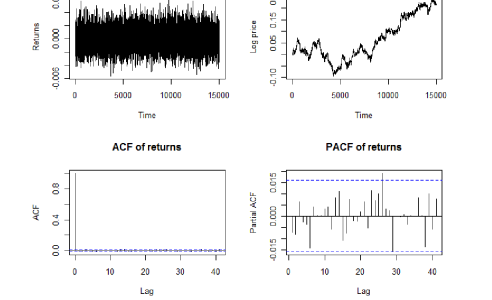
Figure 1: One simulated realization of the calibrated Poisson model (first row in Table 3). Time series plot of returns and log price, as well as ACF and PACF, $n=15000$. The model is calibrated using Boeing’s intensity and Fama/French factor Rm-Rf, such that $\lambda=2.71$, $\sigma=0.0003$, and the mean and standard deviation for the 5-minute returns are $\mu^{*}=3.846\times 10^{-6}$, $\tilde{\sigma}=0.0012$.

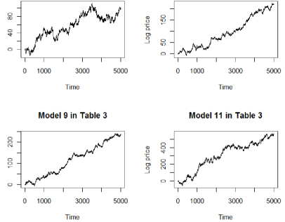
Figure 2: Simulated log price for models in rows 5 ($\mu^{*}=3.846\times 10^{-3}$), 7, 9, and 11 (all with $\mu^{*}=3.846\times 10^{-1}$) of Table 3, $n$=5000.

Parameter values					Size
$n$	$\lambda_{1}=\lambda_{2}$	$\mu_{1}$	$\mu_{2}$	$\mu^{*}$	$T_{1}$	$T_{2}$	$t$
5000	2.71	$4.266\times 10^{-4}$	$-4.266\times 10^{-4}$	0	0.055	0.063	0.045
5000	2.71	$4.173\times 10^{-4}$	$-4.173\times 10^{-4}$	0	0.057	0.050	0.048
5000	2.71	$4.359\times 10^{-4}$	$-4.359\times 10^{-4}$	0	0.048	0.056	0.048
5000	27.1	$4.266\times 10^{-4}$	$-4.266\times 10^{-4}$	0	0.055	0.054	0.052
5000	2.71	0.4266	-0.4266	0	0.043	0.054	0.049
5000	2.71	0.4173	-0.4173	0	0.047	0.055	0.049
5000	2.71	0.3273	-0.3273	0	0.058	0.056	0.053
5000	2.71	0.4359	-0.4359	0	0.061	0.057	0.063
5000	2.71	0.5259	-0.5259	0	0.060	0.058	0.053
5000	27.1	0.4266	-0.4266	0	0.058	0.057	0.046
5000	271	0.4266	-0.4266	0	0.053	0.051	0.058
10000	2.71	0.4173	-0.4173	0	0.050	0.064	0.056
10000	2.71	0.3273	-0.3273	0	0.052	0.051	0.050
10000	2.71	0.4359	-0.4359	0	0.058	0.056	0.057
10000	2.71	0.5259	-0.5259	0	0.060	0.058	0.056

Table 2: Size of the $t$ and $T$ tests for i.i.d. exponential durations.

Parameter values					Power
$n$	$\lambda_{1}=\lambda_{2}$	$\mu_{1}$	$\mu_{2}$	$\mu^{*}$	$T_{1}$	$T_{2}$	$t$
5000	2.71	$4.273\times 10^{-4}$	$-4.259\times 10^{-4}$	$3.846\times 10^{-6}$	0.066	0.077	0.068
5000	2.71	$4.273\times 10^{-4}$	$-4.173\times 10^{-4}$	$3.846\times 10^{-5}$	0.237	0.363	0.575
5000	2.71	$4.359\times 10^{-4}$	$-4.259\times 10^{-4}$	$3.846\times 10^{-5}$	0.242	0.242	0.582
5000	27.1	$4.273\times 10^{-4}$	$-4.259\times 10^{-4}$	$3.846\times 10^{-5}$	0.103	0.105	0.147
5000	2.71	0.4273	-0.4259	$3.846\times 10^{-3}$	0.068	0.089	0.090
5000	2.71	0.4273	-0.4173	$3.846\times 10^{-2}$	0.361	0.615	0.878
5000	2.71	0.4273	-0.3273	$3.846\times 10^{-1}$	1	1	1
5000	2.71	0.4359	-0.4259	$3.846\times 10^{-2}$	0.359	0.593	0.853
5000	2.71	0.5259	-0.4259	$3.846\times 10^{-1}$	1	1	1
5000	27.1	0.4273	-0.4259	$3.846\times 10^{-2}$	0.151	0.204	0.222
5000	271	0.4273	-0.4259	$3.846\times 10^{-1}$	0.357	0.596	0.880
10000	2.71	0.4273	-0.4173	$3.846\times 10^{-2}$	0.492	0.788	0.993
10000	2.71	0.4273	-0.3273	$3.846\times 10^{-1}$	1	1	1
10000	2.71	0.4359	-0.4259	$3.846\times 10^{-2}$	0.461	0.790	0.991
10000	2.71	0.5259	-0.4259	$3.846\times 10^{-1}$	1	1	1

Table 3: Power of the $t$ and $T$ tests for i.i.d. exponential durations.

6.2 ACD durations

We generate $\{\tau_{k}^{(i)}\}$ from the exponential ACD(1,1) model (EACD(1,1)) that satisfies (5.1) with $\{\epsilon_{k}^{(i)}\}\ \stackrel{{\scriptstyle i.i.d.}}{{\sim}}\ exp(1)$, $i=1,2$. We generate models with finite and infinite variance for the durations. For the finite variance model, we try two block sizes $b=160$ and 320. For the EACD(1,1), $t$ is oversized and therefore we will not examine its power. We will also study the size and power of the $T$ tests.

6.2.1 Parameter calibration

Similarly as in Section 6.1, for both finite and infinite variance EACD models, we consider a total of 30 configurations of parameters and sample size, 15 for evaluating size (Table 5 for the finite variance model, Table 7 for the infinite variance model), and 15 for evaluating power (Table 6 for the finite variance model, Table 8 for the infinite variance model). The model has six parameters ($\alpha,\beta,\omega,\sigma,\mu_{1},\mu_{2}$). Note that we assume that $\alpha,\beta,\omega,\sigma$ are the same for both processes $\{\tau_{k}^{(1)}\}$, $\{\tau_{k}^{(2)}\}$.

EACD(1,1) with finite variance

The necessary and sufficient condition for finite variance of the EACD(1,1) model is

$$2\alpha^{2}+\beta^{2}+2\alpha\beta=\alpha^{2}+(\alpha+\beta)^{2}<1\;,$$ (6.4)

For the first configuration corresponding to power (Table 6), we still calibrate the model to match the mean and standard deviation of the returns to those of the Fama/French factor, Rm-Rf, and the ($\alpha,\beta,\omega$) observed in the Boeing series used in Deo et al., (2010), which satisfy (6.4). We use the same $\sigma$ as for the exponential durations and set $\mu_{1}$ and $\mu_{2}$ to match the mean and standard deviation of the Rm-Rf. This calibrated model also accounts for the discrepancies in the time units, and is given in the first row of Table 6. For the EACD(1,1) model, there is no explicit functional relationship between the model parameters and the mean and variance of the calendar-time returns, since these now also depend on the variance of counts (the number of events occurring in a given 5-minute time interval). We estimate the variance of counts using simulation and set $\mu_{1}$ and $\mu_{2}$ accordingly.

Figure 3, for one simulated realization from this model with $n=5000$, shows the time series plots of returns and log price, as well as the ACF and PACF of the returns. Both ACF and PACF show statistically significant autocorrelations at several lags.

For the remaining configurations in Table 6, we increase $\mu^{*}$ by varying $\omega$ (which changes $\lambda$) and $\mu_{i}$. We also consider the two sample sizes, $n=5000$ and $n=10000$. The power should generally increase as $\mu^{*}$ increases. Figure 4 shows the time series plots of the log price for the models of rows 5 ($\mu^{*}=3.846\times 10^{-3}$), 7, 9, and 11 (all with $\mu^{*}=3.846\times 10^{-1}$) of Table 6.

For the first configuration corresponding to size (Table 5), similarly as in Section 6.1.1, we set the mean to zero. For the remaining configurations in these two tables, we vary the $\omega$ and $\mu_{i}$ similarly as in Table 6 while keeping $\mu^{*}=0$.

For each configuration of size and power, we generate 1000 realizations. The simulation procedure is the same as for the exponential durations.

EACD(1,1) with infinite variance

The necessary and sufficient condition for the EACD(1,1) model to have infinite variance is

$$\alpha,\beta\geq 0,\;\;\alpha+\beta<1,\;\;\alpha^{2}+(\alpha+\beta)^{2}\geq 1\;.$$

We fix $\alpha+\beta=0.99$ which is the same as for all of the finite variance models. Table 4 shows the ($\alpha$, $\beta$) values that satisfy the above constraint while attaining the values of $\alpha^{2}+(\alpha+\beta)^{2}$ given in the top row. Since for the ACD model, estimates of $\beta$ are typically close to 1, we choose the first pair $\alpha=0.1729$, $\beta=0.817$. We adjust $\omega$ to obtain the same values of $\lambda$ as used in the finite variance EACD(1,1) models. The value of $\sigma$ is the same as before. Then following the same procedure as described in the finite variance model, we obtain the size (Table 7) and power (Table 8).

Figure 5, for one simulated realization from this model with $n=5000$, shows the time series plots of returns and log price, as well as the ACF and PACF of the returns. Figure 6 shows the time series plots of the log price for the models of rows 5 ($\mu^{*}=3.846\times 10^{-3}$), 7, 9, and 11 (all with $\mu^{*}=3.846\times 10^{-1}$) of Table 8.

We obtained similar results not shown here for other configurations of ($\alpha$, $\beta$, $\omega$) both with and without the constraint $\alpha+\beta=0.99$.

$\alpha^{2}+(\alpha+\beta)^{2}$	1.01	1.02	1.04	1.06	1.08	1.10
$\alpha$	0.1729	0.1997	0.2447	0.28267	0.3161	0.3463
$\beta$	0.8171	0.7903	0.7453	0.7073	0.6739	0.6437

Table 4: ($\alpha$, $\beta$) values such that $\alpha+\beta=0.99$ and $\alpha^{2}+(\alpha+\beta)^{2}$ is given in the top row.

6.2.2 Size/Power of the $t$ and $T$ tests for EACD(1,1) durations

The size for both the finite variance (Table 5) and infinite variance models (Table 7) show that for EACD(1,1) durations, the $t$ test is over-sized and not reliable, especially in the infinite variance cases. Thus, we will not examine the power of the $t$ test here.

For the finite variance cases, the $T$ test is correctly sized. Table 6 indicates that the power of $T$ has the same properties as in the Poisson model, i.e., the power increases as $\mu^{*}$ or $n$ increases; $T_{2}$ generally has higher power than $T_{1}$.

For the infinite variance cases, Table 7 for size shows that both $T_{1}$ and $T_{2}$ are under-sized in some cases and are approximately correctly sized in the other cases. Table 8 shows that the power of both $T_{1}$ and $T_{2}$ increases as $\mu^{*}$ or $n$ increases, but perhaps not as fast as for the finite variance models. $T_{2}$ has higher power than $T_{1}$, particularly when $\mu^{*}$ is large.

The results of Tables 5 and 6 show no apparent sensitivity to the block size.

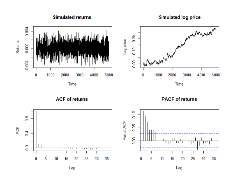
Figure 3: One simulated realization of the calibrated EACD(1,1) model with finite variance (first row in Table 6). Time series plot of returns and log price, as well as ACF and PACF, $n=5000$. The model is calibrated using Boeing’s and Fama/French factor Rm-Rf, such that $\alpha=0.023161$ $\beta=0.970158$, $\omega=0.00247$, $\sigma=0.0003$, and the mean and standard deviation for the 5-minute returns are $\mu^{*}=3.846\times 10^{-6}$, $\tilde{\sigma}=0.0012$.

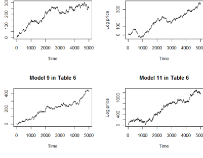
Figure 4: Simulated log price for models in rows 5 ($\mu^{*}=3.846\times 10^{-3}$), 7, 9, and 11 (all with $\mu^{*}=3.846\times 10^{-1}$) of Table 6, $n$=5000.

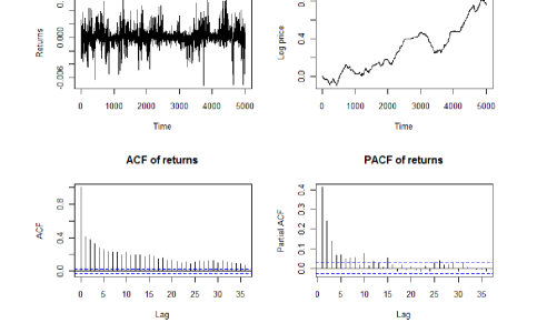
Figure 5: One simulated realization of the calibrated EACD(1,1) model with infinite variance (first row in Table 8). Time series plot of returns and log price, as well as ACF and PACF, $n=5000$. The model is calibrated using Boeing’s and Fama/French factor Rm-Rf, such that $\alpha=0.1729$, $\beta=0.8171$, $\omega=0.00369$, $\sigma=0.0003$, and the mean and standard deviation for the 5-minute returns are $\mu^{*}=3.846\times 10^{-6}$, $\tilde{\sigma}=0.0012$.

Figure 6: Simulated log price for models in rows 5 ($\mu^{*}=3.846\times 10^{-3}$), 7, 9, and 11 (all with $\mu^{*}=3.846\times 10^{-1}$) of Table 8, $n$=5000.

Parameter values						Size ($b=160$)		Size ($b=320$)		Size
$n$	$\omega$	$\lambda_{1}=\lambda_{2}$	$\mu_{1}$	$\mu_{2}$	$\mu^{*}$	$T_{1}$	$T_{2}$	$T_{1}$	$T_{2}$	$t$
5000	0.00247	2.71	$3.380\times 10^{-4}$	$-3.380\times 10^{-4}$	0	0.043	0.043	0.046	0.054	0.165
5000	0.00247	2.71	$3.245\times 10^{-4}$	$-3.245\times 10^{-4}$	0	0.058	0.045	0.057	0.047	0.185
5000	0.00247	2.71	$3.515\times 10^{-4}$	$-3.515\times 10^{-4}$	0	0.043	0.045	0.046	0.048	0.175
5000	0.000247	27.1	$3.380\times 10^{-4}$	$-3.380\times 10^{-4}$	0	0.058	0.057	0.056	0.056	0.171
5000	0.00247	2.71	0.3380	-0.3380	0	0.056	0.057	0.062	0.061	0.222
5000	0.00247	2.71	0.3245	-0.3245	0	0.055	0.045	0.057	0.057	0.232
5000	0.00247	2.71	0.1966	-0.2023	0	0.059	0.049	0.054	0.049	0.248
5000	0.00247	2.71	0.3515	-0.3515	0	0.057	0.052	0.060	0.064	0.250
5000	0.00247	2.71	0.4793	-0.4793	0	0.051	0.053	0.056	0.062	0.228
5000	0.000247	27.1	0.3380	-0.3380	0	0.054	0.050	0.059	0.046	0.233
5000	0.0000247	271	0.3380	-0.3380	0	0.050	0.054	0.050	0.065	0.226
10000	0.00247	2.71	0.3245	-0.3245	0	0.044	0.046	0.047	0.050	0.209
10000	0.00247	2.71	0.1966	-0.1966	0	0.048	0.050	0.043	0.050	0.213
10000	0.00247	2.71	0.3515	-0.3515	0	0.052	0.047	0.060	0.044	0.243
10000	0.00247	2.71	0.4793	-0.4793	0	0.052	0.048	0.055	0.045	0.235

Table 5: Size of the $t$ and $T$ tests for EACD(1,1) durations with finite variance.

Parameter values						Power ($b=160$)		Power ($b=320$)
$n$	$\omega$	$\lambda_{1}=\lambda_{2}$	$\mu_{1}$	$\mu_{2}$	$\mu^{*}$	$T_{1}$	$T_{2}$	$T_{1}$	$T_{2}$
5000	0.00247	2.71	$3.387\times 10^{-4}$	$-3.373\times 10^{-4}$	$3.846\times 10^{-6}$	0.043	0.054	0.052	0.063
5000	0.00247	2.71	$3.387\times 10^{-4}$	$-3.245\times 10^{-4}$	$3.846\times 10^{-5}$	0.175	0.196	0.187	0.203
5000	0.00247	2.71	$3.515\times 10^{-4}$	$-3.373\times 10^{-4}$	$3.846\times 10^{-5}$	0.145	0.193	0.155	0.205
5000	0.000247	27.1	$3.387\times 10^{-4}$	$-3.373\times 10^{-4}$	$3.846\times 10^{-5}$	0.093	0.096	0.095	0.098
5000	0.00247	2.71	0.3387	-0.3373	$3.846\times 10^{-3}$	0.068	0.066	0.067	0.070
5000	0.00247	2.71	0.3387	-0.3245	$3.846\times 10^{-2}$	0.176	0.204	0.178	0.211
5000	0.00247	2.71	0.3387	-0.1966	$3.846\times 10^{-1}$	0.964	1	0.954	0.999
5000	0.00247	2.71	0.3515	-0.3373	$3.846\times 10^{-2}$	0.173	0.219	0.171	0.216
5000	0.00247	2.71	0.4793	-0.3373	$3.846\times 10^{-1}$	0.906	0.999	0.918	0.999
5000	0.000247	27.1	0.3387	-0.3373	$3.846\times 10^{-2}$	0.088	0.089	0.094	0.091
5000	0.0000247	271	0.3387	-0.3373	$3.846\times 10^{-1}$	0.198	0.282	0.190	0.276
10000	0.00247	2.71	0.3387	-0.3245	$3.846\times 10^{-2}$	0.250	0.311	0.253	0.328
10000	0.00247	2.71	0.3387	-0.1966	$3.846\times 10^{-1}$	0.997	1	0.992	1
10000	0.00247	2.71	0.3515	-0.3373	$3.846\times 10^{-2}$	0.230	0.302	0.243	0.335
10000	0.00247	2.71	0.4793	-0.3373	$3.846\times 10^{-1}$	0.972	1	0.962	1

Table 6: Power of the $T$ tests for EACD(1,1) durations with finite variance.

Parameter values						Size
$n$	$\omega$	$\lambda_{1}=\lambda_{2}$	$\mu_{1}$	$\mu_{2}$	$\mu^{*}$	$T_{1}$	$T_{2}$	$t$
5000	0.00369	2.71	$1.848\times 10^{-4}$	$-1.848\times 10^{-4}$	0	0.040	0.041	0.393
5000	0.00369	2.71	$1.713\times 10^{-4}$	$-1.713\times 10^{-4}$	0	0.043	0.044	0.409
5000	0.00369	2.71	$1.983\times 10^{-4}$	$-1.983\times 10^{-4}$	0	0.041	0.040	0.439
5000	0.000369	27.1	$1.848\times 10^{-4}$	$-1.848\times 10^{-4}$	0	0.042	0.041	0.372
5000	0.00369	2.71	0.1848	-0.1848	0	0.041	0.042	0.448
5000	0.00369	2.71	0.1713	-0.1713	0	0.043	0.040	0.417
5000	0.00369	2.71	0.0435	-0.0435	0	0.060	0.054	0.571
5000	0.00369	2.71	0.1983	-0.1983	0	0.046	0.043	0.448
5000	0.00369	2.71	0.3261	-0.3261	0	0.053	0.059	0.506
5000	0.000369	27.1	0.1848	-0.1848	0	0.043	0.041	0.385
5000	0.0000369	271	0.1848	-0.1848	0	0.045	0.045	0.379
10000	0.00369	2.71	0.1713	-0.1713	0	0.045	0.040	0.435
10000	0.00369	2.71	0.0435	-0.0435	0	0.055	0.047	0.536
10000	0.00369	2.71	0.1983	-0.1983	0	0.043	0.042	0.453
10000	0.00369	2.71	0.3261	-0.3261	0	0.046	0.051	0.517

Table 7: Size of the $t$ and $T$ tests for EACD(1,1) durations with infinite variance.

Parameter values						Power
$n$	$\omega$	$\lambda_{1}=\lambda_{2}$	$\mu_{1}$	$\mu_{2}$	$\mu^{*}$	$T_{1}$	$T_{2}$
5000	0.00369	2.71	$1.855\times 10^{-4}$	$-1.841\times 10^{-4}$	$3.846\times 10^{-6}$	0.041	0.042
5000	0.00369	2.71	$1.855\times 10^{-4}$	$-1.713\times 10^{-4}$	$3.846\times 10^{-5}$	0.060	0.056
5000	0.00369	2.71	$1.983\times 10^{-4}$	$-1.841\times 10^{-4}$	$3.846\times 10^{-5}$	0.046	0.047
5000	0.000369	27.1	$1.855\times 10^{-4}$	$-1.841\times 10^{-4}$	$3.846\times 10^{-5}$	0.042	0.043
5000	0.00369	2.71	0.1855	-0.1841	$3.846\times 10^{-3}$	0.046	0.044
5000	0.00369	2.71	0.1855	-0.1713	$3.846\times 10^{-2}$	0.047	0.046
5000	0.00369	2.71	0.1855	-0.0435	$3.846\times 10^{-1}$	0.408	0.622
5000	0.00369	2.71	0.1983	-0.1841	$3.846\times 10^{-2}$	0.056	0.058
5000	0.00369	2.71	0.3261	-0.1841	$3.846\times 10^{-1}$	0.244	0.299
5000	0.000369	27.1	0.1855	-0.1841	$3.846\times 10^{-2}$	0.044	0.045
5000	0.0000369	271	0.1855	-0.1841	$3.846\times 10^{-1}$	0.057	0.059
10000	0.00369	2.71	0.1855	-0.1713	$3.846\times 10^{-2}$	0.043	0.046
10000	0.00369	2.71	0.1855	-0.0435	$3.846\times 10^{-1}$	0.453	0.682
10000	0.00369	2.71	0.1983	-0.1841	$3.846\times 10^{-2}$	0.050	0.052
10000	0.00369	2.71	0.3261	-0.1841	$3.846\times 10^{-1}$	0.258	0.358

Table 8: Power of the $T$ tests for EACD(1,1) durations with infinite variance.

6.3 LMSD durations

We generate $\{\tau_{k}^{(i)}\}$ from the LMSD model

$$\tau_{k}=\epsilon_{k}e^{Y_{k}}$$

where $\{\epsilon_{k}\}\ \stackrel{{\scriptstyle i.i.d.}}{{\sim}}\ Weibull(\delta,\gamma)$, and ($\delta$, $\gamma$) are the scale and shape parameter; $\{Y_{k}\}$ is a Gaussian ARFIMA$(1,d,0)$ process with innovations $w_{k}\ \stackrel{{\scriptstyle i.i.d.}}{{\sim}}\ N(0,\sigma_{w}^{2})$, given by

$$(1-\alpha L)(1-L)^{d}Y_{k}=w_{k}$$

with $|\alpha|<1$, and $d$ is the long memory parameter with $d=H-1/2\in(0,1/2)$. We generate models without and with microstructure shocks $\{\eta_{k}\}$. For all of these models, we find that $t$ is oversized and therefore we will not examine its power. We will also study the size and power of the $T$ tests and the leverage effect induced by the microstructure shocks. In all simulations, we use 1000 realizations and block size $b=160$.

6.3.1 Parameter calibration

For both LMSD models without and with $\{\eta_{k}\}$, we consider a total of 30 configurations of parameters and sample size, 15 for evaluating size (Table 10), and 15 for evaluating power (Table 11). Parameters for the LMSD model are ($\alpha$, $\delta$, $\gamma$, $\sigma_{w}^{2}$, $d$, $\sigma$, $\mu_{1}$, $\mu_{2}$). Note that we assume that ($\alpha$, $\delta$, $\gamma$, $\sigma_{w}^{2}$, $d$, $\sigma$) are the same for both processes $\{\tau_{k}^{(1)}\}$, $\{\tau_{k}^{(2)}\}$.

LMSD without microstructure shocks

For the first configuration corresponding to power (Table 11), we calibrate the model to match the ($\alpha,\delta,\gamma,\sigma_{w}^{2},d$) observed in the Boeing series used in Deo et al., (2010). We use the same $\sigma$ as for the exponential durations and set $\mu_{1}$ and $\mu_{2}$ to match the mean and standard deviation of the Rm-Rf. This calibrated model also accounts for the discrepancies in the time units, and is given in the first row of Table 11. Similarly as for the EACD(1,1) model, for the LMSD model, the functional relationship between the model parameters and the mean and variance of the calendar-time returns also depend on the variance of counts. We estimate the variance of counts using simulation and set $\mu_{1}$ and $\mu_{2}$ accordingly. Figure 7, for one simulated realization from this model with $n=5000$, shows the time series plots of returns and log price, as well as the ACF and PACF of the returns.

For the remaining configurations in Table 11, we increase $\mu^{*}$ by varying $\delta$ (which changes $\lambda$) and $\mu_{i}$. We consider two sample sizes, $n=5000$ and $n=10000$. The power should generally increase as $\mu^{*}$ increases.

For the first configuration corresponding to size (Table 10), we set the mean to zero. For the remaining configurations in these two tables, we vary the $\delta$ and $\mu_{i}$ similarly as in Table 11 while keeping $\mu^{*}=0$.

LMSD with microstructure shocks

For $i=1,2$, define the microstructure shock $\eta_{k}$ as

$$\eta_{k}=Y_{k-1}-Y_{k}\;.$$

With $\{\eta_{k}\}$, the functional relationship between the model parameters and the variance of the calendar-time returns now depend on not only the variance of counts, but also the variance of $\{\eta_{k}\}$ and the covariance of counts and $\{\eta_{k}\}$. Since it is difficult to calibrate this variance and covariance, for simplicity, we will use the same values of all parameters ($\alpha$, $\delta$, $\gamma$, $\sigma_{w}^{2}$, $d$, $\sigma$, $\mu_{1}$, $\mu_{2}$) as those used in the LMSD models without $\{\eta_{k}\}$. The size and power results are given in Tables 10 (size) and 11 (power).

Figure 8, for one simulated realization from first configuration of Table 11 with $\{\eta_{k}\}$, shows the time series plots of returns and log price, as well as the ACF and PACF of the returns. Figure 9 shows the time series plots of the log price for the models with $\{\eta_{k}\}$ of rows 5 ($\mu^{*}=3.846\times 10^{-3}$), 7, 9, and 11 (all with $\mu^{*}=3.846\times 10^{-1}$) in Table 11.

6.3.2 Leverage effect

In model (2.1), we assume that the microstructure shocks $\{\eta_{i,k}\}$ are independent of the efficient shocks $\{e_{1,k}\}$, $\{e_{2,k}\}$, but not necessarily of the counting process $(N_{1},N_{2})$. This allows for a leverage effect. See Aue et al., (2014). The leverage is then defined as the correlation between current calendar-time return $r_{k}$ and absolute value of the next calendar-time return $|r_{k+1}|$

$$leverage=corr(r_{k},|r_{k+1}|)\;.$$

We test the model with different memory parameter $d=.23$ and $d=.4$, keeping other parameters the same as in the first configuration of Table 11. We generate 100 realizations, with $n=5000$, calculate sample leverage for each realization, and use the $t$-test for the mean,

$$H_{0}:\;leverage=0$$

$$H_{1}:\;leverage<0\;.$$

Table 9 shows the mean of sample leverage and the $p$-value for models with different memory parameters $d$. Without the $\{\eta_{k}\}$, there is no leverage in returns, while including the $\{\eta_{k}\}$ can induce a leverage effect, i.e. negative correlation between current return and the next period’s absolute return.

Model	$d=0.23$		$d=0.4$
	Mean	p-value	Mean	p-value
Returns without $\eta_{k}$	0.00062	0.6265	-0.00374	0.3727
Returns with $\eta_{k}$	-0.02299	0.0000	-0.01883	0.0000

Table 9: Means and p-values of sample leverage for models with $d=.23$ and $d=.4$.

6.3.3 Size/Power of the $t$ and $T$ tests for LMSD durations

Tables 10 and 11 show that there is no significant difference in the size and power between models without and with microstructure shocks $\{\eta_{k}\}$. For both models, Table 10 shows that the $t$ test is oversized. $T_{1}$ is correctly sized in all cases, while $T_{2}$ is a bit oversized. As we increase $\lambda$ or $n$, the size of $T_{2}$ becomes smaller. Table 11 shows that the power of the $T$ test performs similarly as in the Poisson model: the power increases as $\mu^{*}$ increases; as $n$ is increased holding all model parameters fixed, the power increases; $T_{2}$ has higher power than $T_{1}$.

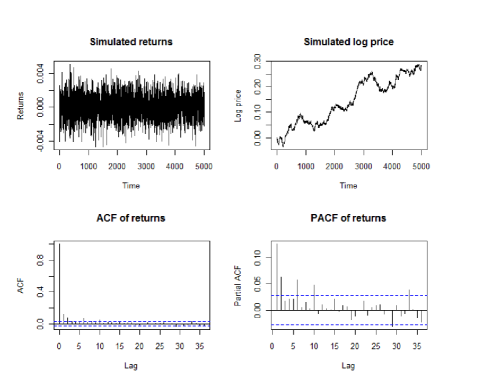
Figure 7: One simulated realization of the calibrated LMSD model without $\{\eta_{k}\}$ (first row in Table 11). Time series plot of returns and log price, as well as ACF and PACF, $n$=5000. The model is calibrated using Boeing’s and Fama/French factor Rm-Rf, such that $\alpha=-.4212$, $\delta=0.2$, $\gamma=1.3376$, $\sigma_{w}^{2}=0.2368$, $d=0.3545$, $\sigma=0.0003$, and the mean and standard deviation for the 5-minute returns are $\mu^{*}=3.846\times 10^{-6}$, $\tilde{\sigma}=0.0012$.

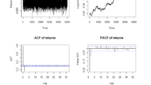
Figure 8: One simulated realization of the calibrated LMSD model with $\{\eta_{k}\}$ (first row in Table 11). Time series plot of returns and log price, as well as ACF and PACF, $n$=5000. The model is calibrated using Boeing’s and Fama/French factor Rm-Rf, such that $\alpha=-.4212$, $\delta=0.2$, $\gamma=1.3376$, $\sigma_{w}^{2}=0.2368$, $d=0.3545$, $\sigma=0.0003$, and the mean and standard deviation for the 5-minute returns are $\mu^{*}=3.846\times 10^{-6}$, $\tilde{\sigma}=0.0012$.

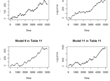
Figure 9: Simulated log price for models with $\{\eta_{k}\}$ in rows 5 ($\mu^{*}=3.846\times 10^{-3}$), 7, 9, and 11 (all with $\mu^{*}=3.846\times 10^{-1}$) of Table 11.

Parameter values						Size (without $\eta_{k}$)			Size (with $\eta_{k}$)
$n$	$\delta$	$\lambda_{1}=\lambda_{2}$	$\mu_{1}$	$\mu_{2}$	$\mu^{*}$	$T_{1}$	$T_{2}$	$t$	$T_{1}$	$T_{2}$	$t$
5000	0.2	4.58	$2.293\times 10^{-4}$	$-2.293\times 10^{-4}$	0	0.057	0.071	0.307	0.051	0.080	0.307
5000	0.2	4.58	$2.213\times 10^{-4}$	$-2.213\times 10^{-4}$	0	0.059	0.080	0.312	0.057	0.084	0.311
5000	0.2	4.58	$2.373\times 10^{-4}$	$-2.373\times 10^{-4}$	0	0.052	0.064	0.291	0.061	0.079	0.320
5000	0.02	45.8	$2.293\times 10^{-4}$	$-2.293\times 10^{-4}$	0	0.052	0.083	0.337	0.059	0.072	0.314
5000	0.2	4.58	0.2293	-0.2293	0	0.058	0.073	0.341	0.061	0.063	0.345
5000	0.2	4.58	0.2213	-0.2213	0	0.063	0.088	0.352	0.057	0.089	0.351
5000	0.2	4.58	0.1458	-0.1458	0	0.046	0.073	0.376	0.044	0.081	0.341
5000	0.2	4.58	0.2373	-0.2373	0	0.057	0.078	0.366	0.053	0.076	0.339
5000	0.2	4.58	0.3129	-0.3129	0	0.056	0.077	0.343	0.062	0.077	0.372
5000	0.02	45.8	0.2293	-0.2293	0	0.052	0.070	0.357	0.054	0.071	0.364
5000	0.002	458	0.2293	-0.2293	0	0.054	0.057	0.371	0.053	0.052	0.389
10000	0.2	4.58	0.2213	-0.2213	0	0.057	0.068	0.366	0.062	0.070	0.368
10000	0.2	4.58	0.1458	-0.1458	0	0.053	0.070	0.368	0.056	0.071	0.370
10000	0.2	4.58	0.2373	-0.2373	0	0.048	0.071	0.368	0.051	0.070	0.376
10000	0.2	4.58	0.3129	-0.3129	0	0.052	0.071	0.373	0.051	0.071	0.374

Table 10: Size of the $t$ and $T$ tests for LMSD durations.

Parameter values						Power (without $\eta_{k}$)		Power (with $\eta_{k}$)
$n$	$\delta$	$\lambda_{1}=\lambda_{2}$	$\mu_{1}$	$\mu_{2}$	$\mu^{*}$	$T_{1}$	$T_{2}$	$T_{1}$	$T_{2}$
5000	0.2	4.58	$2.297\times 10^{-4}$	$-2.289\times 10^{-4}$	$3.846\times 10^{-6}$	0.072	0.080	0.071	0.090
5000	0.2	4.58	$2.297\times 10^{-4}$	$-2.213\times 10^{-4}$	$3.846\times 10^{-5}$	0.134	0.202	0.128	0.197
5000	0.2	4.58	$2.373\times 10^{-4}$	$-2.289\times 10^{-4}$	$3.846\times 10^{-5}$	0.116	0.161	0.130	0.204
5000	0.02	45.8	$2.297\times 10^{-4}$	$-2.289\times 10^{-4}$	$3.846\times 10^{-5}$	0.076	0.092	0.075	0.087
5000	0.2	4.58	0.2297	-0.2289	$3.846\times 10^{-3}$	0.074	0.08	0.067	0.069
5000	0.2	4.58	0.2297	-0.2213	$3.846\times 10^{-2}$	0.139	0.193	0.120	0.192
5000	0.2	4.58	0.2297	-0.1458	$3.846\times 10^{-1}$	0.881	0.999	0.905	0.998
5000	0.2	4.58	0.2373	-0.2289	$3.846\times 10^{-2}$	0.141	0.193	0.107	0.166
5000	0.2	4.58	0.3129	-0.2289	$3.846\times 10^{-1}$	0.697	0.965	0.688	0.974
5000	0.02	45.8	0.2297	-0.2289	$3.846\times 10^{-2}$	0.079	0.089	0.062	0.080
5000	0.002	458	0.2297	-0.2289	$3.846\times 10^{-1}$	0.091	0.105	0.083	0.098
10000	0.2	4.58	0.2297	-0.2213	$3.846\times 10^{-2}$	0.154	0.209	0.144	0.204
10000	0.2	4.58	0.2297	-0.1458	$3.846\times 10^{-1}$	0.940	1	0.949	1
10000	0.2	4.58	0.2373	-0.2289	$3.846\times 10^{-2}$	0.145	0.205	0.143	0.195
10000	0.2	4.58	0.3129	-0.2289	$3.846\times 10^{-1}$	0.793	0.997	0.780	0.990

Table 11: Power of the $T$ tests for LMSD durations.

7 Data analysis

We study the daily returns of the Fama/French factor, Rm-Rf, from Kenneth French’s data library. According to the website, “Rm-Rf is the excess return on the market, value-weight return of all CRSP (Center for Research in Security Prices) firms incorporated in the US and listed on the NYSE, AMEX, or NASDAQ that have a CRSP share code of 10 or 11 at the beginning of month t, good shares and price data at the beginning of t, and good return data for t minus the one-month Treasury bill rate (from Ibbotson Associates)”(http://mba.tuck.dartmouth.edu/pages/faculty/ken.french/data_library.html). The data ranges from July 1, 1926 to December 31, 2013, a total 23133 daily excess returns with sample mean 0.000285.

Figure 10 shows the time series plot, log price, ACF and PACF of daily excess returns. Both ACF and PACF show statistically significant lags. We perform a $t$-test based on the usual standard error and the Newey-West standard error, which allows for serial correlation, and also our $T_{1}$ test for the following hypothesis:

$$H_{0}:\mu^{*}=0$$

$$H_{1}:\mu^{*}>0$$

where $\mu^{*}$ is the expected excess return (equity premium). To conduct the $T_{1}$ test, we calculate the $T_{1}$ statistic for the entire data set, and use the same subsampling procedure as defined in Section 6 to obtain the empirical quantiles of the limiting distribution of T. As suggested by Jach et al., (2012), with the sample size of $n=23133$, we consider the block size $b\in\{732,976,1302,1736,2314,3086,4116,5488\}$. This covers subsample sizes ranging from $3-24\%$ of the sample size. The results are given in Table 12.

At the 0.05 significant level, both the ordinary $t$-test and the Newey-West $t$-test reject the null hypothesis with very small p-values, 2.59e-05 and 7.40e-05 respectively. This seems to provide extremely strong evidence for an equity premium. However, the much larger $p$-values for all of the $T_{1}$ tests considered indicate far weaker evidence against the null hypothesis. This finding is consistent with the simulation results in Section 6 for the EACD and LMSD durations. The $p$-values corresponding to the ordinary $t$-tests may be spuriously low, and the ones corresponding to the $T_{1}$ tests may be more reliable.

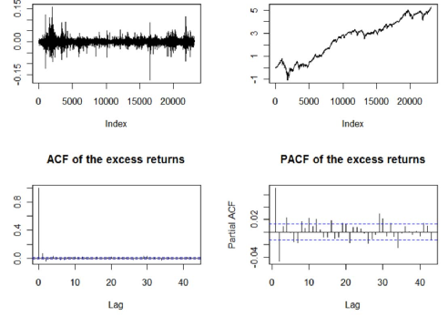
Figure 10: Time series plot, log price, ACF, and PACF of daily excess returns from July 1, 1926 to December 31, 2013.

T test
Block size (b)	732	977	1302	1736
$p$-value	0.054	0.057	0.056	0.058
Block size (b)	2351	3087	4117	5489
$p$-value	0.064	0.062	0.065	0.057

Table 12: $T_{1}$ test results for daily excess returns Rm-Rf.

8 Discussion: Long Memory and Heavy Tails of Stock Returns

The introduction of a nonzero mean in the efficient shocks in the model (2.1) provides a link by which properties of intertrade durations can affect those of certain quantities that are observed at a macroscopic level. We have focused so far on inference for the trend (based on studying the asymptotic distribution of the log price). To illustrate just one of the variety of possible additional quantities of interest, we now turn our attention to properties of returns.

Lo, (1991) investigated whether stock returns have long memory, and Mandelbrot, (1963) argued that returns have infinite variance. Both of these propositions have met with considerable controversy, but under the model (2.2) both could contain an important grain of truth. Generalizing the analysis presented so far leads to a more nuanced interpretation of what these propositions could mean.

From here on in this section, when we mention sequences of random variables, we allow for suitable renormalization (centering and scaling) without always specifically mentioning or writing the renormalization. So the discussion here is somewhat informal, but can be made mathematically rigorous. We focus here on the case $\gamma>1/2$.

Proposition 2.1 implies that partial sums of returns (after suitable renormalization) converge in distribution to a random variable that need not be Gaussian. This theorem has allowed us to discuss issues related to inference for the slope parameter, which is the expectation of the average return. It is also of interest to ask if one can go further and say something about the joint distribution of the returns themselves, rather than their sum. Therefore, we will now discuss the joint limiting distribution of any fixed number of contiguous returns at long horizons.

Although we have so far taken the time spacing in defining the returns to be 1, there is no essential reason for this and here we replace it by an arbitrary $T>0$, and we define the returns with respect to this time spacing as $r_{j,T}=y(jT)-y((j-1)T)$. Now consider the first $M$ of these returns, where $M$ is fixed. It follows from our assumptions here (by arguments similar to the proof of Proposition 2.1 and by Theorem 7.3.2 of Whitt, (2002)) that the joint distribution of these $M$ returns (after suitable renormalization) converges as $T\rightarrow\infty$ to the distribution of $M$ contiguous increments of the limiting process.

In our LMSD example, assuming finite variance and an exponential volatility function, the limiting process is fractional Brownian motion. Thus in this case, the $M$ returns converge in distribution to $M$ contiguous observations of a fractional Gaussian noise. In this sense, it could be said that the returns (computed at a sufficiently high level of aggregation) have long memory. Simulations not shown here of the model (2.2) in this LMSD case show that it may be hard to detect this long memory due to the additive noise that arises from the second term on the righthand side of (2.2).

In the ACD example (and certain cases of the LMSD example as well), it turns out that the limiting process can be a stable process, for which the increments are independent and have infinite-variance stable distributions. So here, our $M$ long-horizon returns converge in distribution (as $T\rightarrow\infty$, and after suitable renormalization) to a sequence of $M$ i.i.d. stable random variables. This would seem to correspond to the proposition that returns have infinite variance. But actually, the truth here may be more subtle. It can happen that, for each fixed $T$ the variance of the returns is finite. See, for example, Whitt, (2002) for the underlying point process theory under heavy-tailed durations. It is even possible to construct an example where durations have finite variance and still the limit of partial sums of durations is a stable process, so the returns would once again have finite variance but converge in distribution to i.i.d. stable random variables with infinite variance. Such an example may come from durations that obey a positive version of the renewal-reward process discussed in Taqqu and Levy, (1986) (see also Hsieh et al., (2007)). In such a model, durations would have finite variance but their sums would converge to a process with infinite variance.

In the case where the limiting process is a Lévy-stable process, it is of interest to note that such continuous-time processes have discontinuities with probability 1. These may correspond to what practitioners refer to as ”jumps” in the log price process, even though under our model the log price process is a pure-jump process so that all activity consists of jumps.

The main message of this paper is that even in the simple transaction-level model (2.1) there is a wide variety of possible behaviors of macroscopic quantities of interest. Some additional quantities we hope to study in future work based on this and similar models include: regression coefficients as used in the market model, estimated cointegrating parameters (which were considered without a trend term in Aue et al., (2014)), and sample autocorrelations.

9 Proofs

Proof of Proposition 2.1.

We start by proving the convergences (2.5) and (2.6). Defining $\zeta_{i,k}=e_{i,k}+\eta_{i,k}$, we can write

$$y(n)-\mu^{*}n=\mu_{1}\{N_{1}(n)-\lambda_{1}n\}+\mu_{2}\{N_{2}(n)-\lambda_{2}n\}+\sum_{k=1}^{N_{1}(n)}\zeta_{1,k}+\sum_{k=1}^{N_{2}(n)}\zeta_{2,k}$$

Assumption 2.1 implies that $N_{i}(n)/n{\ \stackrel{{\scriptstyle\mathbb{P}}}{{\to}}}\ \lambda_{i}$. For $t\geq 0$, define $x_{i,n}(t)=n^{-1/2}\sum_{k=1}^{N_{i}(nt)}\zeta_{i,k}$. The present assumptions imply assumptions 2.1, 2.2, 2.3 and 2.4 of Aue et al., (2014), thus Theorem 3.1 therein implies that 0 $x_{i,n}\ \stackrel{{\scriptstyle fi.di.}}{{\longrightarrow}}\ \sqrt{\lambda}\sigma_{i}B_{i}$, where $B_{i}$ are mutually independent standard Brownian motions. Since the sequences $\{e_{i,k}\}$ are independent of the point processes $N_{i}$, the sequences of processes $x_{i,n}$ and $\{n^{-\gamma}(N_{i}(nt)-n\lambda_{i}t),t\geq 0\}$, $i=1,2$ converge jointly. Thus, if $\gamma>1/2$, (2.5) holds and if $\gamma=1/2$, (2.6) holds with $\sigma^{2}=\lambda_{1}\sigma_{1}^{2}+\lambda_{2}\sigma_{2}^{2}$. ∎

Proof of Theorem 3.1.

The convergence (3.3) is a straightforward consequence of Proposition 2.1 and the continuous mapping Theorem. If $\mu^{*}\neq\mu^{*}_{0}$, write

$$T_{n}=\frac{\bar{r}(n)-\mu^{*}}{|\bar{r}(n)-\bar{r}(n/2)|}+\frac{\mu^{*}-\mu_{0}^{*}}{|\bar{r}(n)-\bar{r}(n/2)|}\;.$$

The first term converges weakly to $A(1)/|A(1)-2A(1/2)|$ and the second term converges in probability to $+\infty$ if $\mu^{*}>\mu_{0}^{*}$ and to $-\infty$ if $\mu^{*}<\mu_{0}^{*}$. ∎

Proof of Lemma 3.1.

$$s_{n}^{2}=\frac{1}{n-1}\sum_{j=1}^{n}(r_{j}-\mu^{*})^{2}+\frac{n}{n-1}(\bar{r}_{n}-\mu^{*})^{2}+2(\mu^{*}-\bar{r})\sum_{j=1}^{n}(r_{j}-\mu^{*})$$ (9.1)

Under Assumption 2.1, the convergences (2.5) and (2.6) imply that the second term in (9.1) is $o_{P}(1)$. Since

$$r_{j}-\mu^{*} =\sum_{i=1}^{2}\sum_{k=N_{i}(j-1)+1}^{N_{i}(j)}(\mu_{i}+\zeta_{i,k})-\lambda_{i}\mu_{i}\;,$$

by Assumption (3.1), ergodicity of the marked point processes and mutual independence, we have

$$\frac{1}{n}\sum_{j=1}^{n}(r_{j}-\lambda\mu)^{2}{\ \stackrel{{\scriptstyle\mathbb{P}}}{{\to}}}\ \sum_{i=1}^{2}{\mathbb{E}}\left[\left(\sum_{k=1}^{N_{i}(1)}(\mu_{i}+\zeta_{i,k})-\lambda_{i}\mu_{i}\right)^{2}\right]\;.$$

Since the last term in (9.1) is a cross product, it is therefore also $o_{P}(1)$. ∎

Lemma 9.1.

Let $\xi$ be a stationary random measure such that $n^{-\gamma}\{\xi(nt)-\lambda nt\}\ \stackrel{{\scriptstyle fi.di.}}{{\longrightarrow}}\ A(t)$. Let $N$ be a Cox process with stochastic intensity $\xi$. Then $n^{-\gamma}\{N(nt)-\lambda nt\}\ \stackrel{{\scriptstyle fi.di.}}{{\longrightarrow}}\ A(t)$.

Proof.

We only prove the convergence in distribution of $n^{-\gamma}\{\xi(n)-\lambda n\}$ to $A(1)$. The convergence of the finite dimensional distribution is proved similarly. By conditioning on $\xi$, we have, for all $z\in{\mathbb{R}}$,

$${\mathbb{E}}\left[{\mathrm{e}}^{{\mathrm{i}}zt^{-\gamma}\{N(t)-\lambda t\}}\right] ={\mathbb{E}}\left[{\mathrm{e}}^{\xi(t)\{{\mathrm{e}}^{{\mathrm{i}}zt^{-\gamma}}-1\}-{\mathrm{i}}zt^{1-\gamma}}\right]$$

$$={\mathbb{E}}\left[{\mathrm{e}}^{{\mathrm{i}}zt^{-\gamma}\{\xi(t)-\lambda t\}}\right]+{\mathbb{E}}\left[{\mathrm{e}}^{{\mathrm{i}}zt^{-\gamma}\{\xi(t)-\lambda t\}}\left\{{\mathrm{e}}^{\xi(t)\{{\mathrm{e}}^{{\mathrm{i}}zt^{-\gamma}}-1-{\mathrm{i}}zt^{-\gamma}\}}-1\right\}\right]$$

$$=\phi_{t}(z)+{\rm rest}_{t}(z)\;.$$

By assumption, $\lim_{t\to\infty}\phi_{t}(z)={\mathbb{E}}[{\mathrm{e}}^{{\mathrm{i}}zA(1)}]$. Then, denoting $h(t,z)={\mathrm{e}}^{{\mathrm{i}}zt^{-\gamma}}-1-{\mathrm{i}}zt^{-\gamma}$, the remainder term is bounded by

$$|{\rm rest}_{t}(z)|\leq{\mathbb{E}}\left[\left|{\mathrm{e}}^{h(t,z)\xi(t)}-1\right|\right]\;.$$

For each $z$, $h(t,z)=O(t^{-2\gamma})$, so the assumption on $\xi$ implies that ${\mathrm{e}}^{h(t,z)\xi(t)}-1{\ \stackrel{{\scriptstyle\mathbb{P}}}{{\to}}}\ 0$. Moreover, for all $t>0$ and $z\in{\mathbb{R}}$, $|{\mathrm{e}}^{h(t,z)\xi(t)}-1|\leq 1+{\mathrm{e}}^{(cos(z)-1)\xi(t)}\leq 2$. Thus, the bounded convergence theorem yields that $\lim_{t\to\infty}{\mathbb{E}}[|{\mathrm{e}}^{h(t,z)\xi(t)}-1|]=0$. ∎

We recall the definition of $\theta$-weak dependence from Bardet et al., (2008). For each positive integer $v$, let ${\mathbb{R}}^{v}$ be equipped with the $l^{1}$-norm

$$\|\mathbf{x}-\mathbf{y}\|_{1}=\sum\limits_{i=1}^{v}|x_{i}-y_{i}|,\;\mathbf{x},\mathbf{y}\in{\mathbb{R}}^{v}\;.$$

Let $\mathcal{G}_{v}$ be the class of bounded functions $g:{\mathbb{R}}^{v}\rightarrow{\mathbb{R}}$ such that

$$\mathrm{Lip}(g)=\sup_{\mathbf{x}\neq\mathbf{y}}\frac{|g(\mathbf{x})-g(\mathbf{y})|}{\|\mathbf{x}-\mathbf{y}\|_{1}}<\infty\;.$$

The quantity in the left hand side is denoted $\mathrm{Lip}(g)$ and called the Lipschitz modulus of $g$. A stationary sequence $\{X_{k},k\in{\mathbb{Z}}\}$ is said to be $\theta$ weakly dependent with rate $\{\theta_{k},k\geq 0\}$ if for any $u,v\in\mathbb{N}^{*}$, $(i_{1},\dots,i_{u})\in{\mathbb{Z}}$, $(j_{1},\dots,j_{v})\in{\mathbb{Z}}$ with $i_{1}<\dots<i_{u}\leq i_{u}+k\leq j_{1}<\cdots<j_{v}$, and $f\in\mathcal{G}_{u}$, $g\in\mathcal{G}_{v}$,

$${\mathrm{cov}}(f(r_{i_{1}},\dots,r_{i_{u}}),g(r_{j_{1}},\dots,r_{j_{v}}))\leq v\,\|f\|_{\infty}\,\mathrm{Lip}(g)\,\theta_{k}\;.$$

Lemma 9.2.

Let $N$ be a Cox process with stochastic intensity $\xi$, where

$$\xi(A)=\int_{A}w(s){\mathrm{d}}s\;,$$

and $w$ is a positive stationary stochastic process with almost surely continuous paths. Assume that $w$ is $\theta$-weak dependent. Then

1. the increments $\{\Delta N(k),k\in{\mathbb{Z}}\}$ is $\theta$-weak dependent with the same rate function as the process $w$;

2. If the efficient shocks $e_{i}$ are i.i.d. and independent of the point process $N$, the sequence of calendar-time returns $\{r_{k},k\in\mathbb{N}^{*}\}$, defined by

   $$r_{k}=\sum\limits_{n=N(k-1)+1}^{N(k)}e_{n}\;,$$

   is $\theta$-weak dependent, with the same rate as $w$.

Proof.

Since (i) is a particular case of (ii) with the shocks taken to be uniformly equal to 1, we only need to prove (ii). Let $f\in\mathcal{G}_{u}$ and $g\in\mathcal{G}_{v}$. Consider now the sequence of returns $\{r_{k},k\in\mathbb{N}^{*}\}$. By conditioning on the stochastic intensity, we have

$${\mathrm{cov}}(f(r_{i_{1}},\dots,r_{i_{u}}),g(r_{j_{1}},\dots,r_{j_{v}})) ={\mathbb{E}}\left[{\mathrm{cov}}(f(r_{i_{1}},\dots,r_{i_{u}}),g(r_{j_{1}},\dots,r_{j_{v}}))\mid\xi\right]$$

$$+{\mathrm{cov}}\left({\mathbb{E}}(f(r_{i_{1}},\dots,r_{i_{u}})|\xi),{\mathbb{E}}(g(r_{j_{1}},\dots,r_{j_{v}})|\xi)\right)$$

Since the intervals are non intersecting, and $\{e_{k}\}$ is independent of $N$ which is a Poisson point process conditionally on $\xi$, we have

$${\mathbb{E}}\left({\mathrm{cov}}(f(r_{i_{1}},\dots,r_{i_{u}}),g(r_{j_{i}},\dots,r_{j_{v}})|\xi)\right)=0\;.$$

To compute the second term, denote $h_{n}(x)=\frac{e^{-x}x^{n}}{n!}$ and let $\{e_{k}^{(i)}\}$, $i\in\mathbb{N}$ be i.i.d. copies of the sequence $\{e_{k}\}$ and define $S_{i}(0)=0$ and $S_{i}(n)=\sum_{k=1}^{n}e_{k}^{(i)}$. Denote also $\xi_{i}=\xi(i-1,i]$. Then, by the independent increments property, we have

$${\mathbb{E}}\left[f(r_{i_{1}},\dots,r_{i_{u}})|\xi\right] ={\mathbb{E}}\left[f\left(\sum_{k=N(i_{1}-1)+1}^{N(i_{1})}e_{k},\dots,\sum_{k=N(i_{u}-1)+1}^{N(i_{u})}e_{k}\right)\middle|\xi\right]$$

$$=\sum_{n_{1},\dots,n_{u}=0}^{\infty}{\mathbb{E}}[f(S_{1}(n_{1}),\dots,S_{u}(n_{u}))]\prod_{i=1}^{n}h_{n_{i}}(\xi_{i})\;.$$

Similarly, we have

$${\mathbb{E}}\left(g(r_{j_{1}},\dots,r_{j_{v}})|\xi\right)=\sum\limits_{m_{1},\dots,m_{v}=0}^{\infty}{\mathbb{E}}\left[g(S_{1}(m_{1}),\dots,S_{v}(m_{v}))\right]\prod\limits_{q=1}^{v}h_{m_{q}}(\xi_{j_{q}})\;.$$

Define the functions $F$ and $G$ on ${\mathbb{R}}^{u}$ and ${\mathbb{R}}^{v}$ respectively by

$$F(x_{1},\dots,x_{u}) =\sum_{n_{1},\dots,n_{u}=0}^{\infty}{\mathbb{E}}\left[f(S_{1}(n_{1}),\dots,S_{u}(n_{u}))\right]\prod\limits_{i=1}^{u}h_{n_{i}}(x_{i})\;,$$

$$G(x_{1},\dots,x_{v}) =\sum_{m_{1},\dots,m_{v}=0}^{\infty}{\mathbb{E}}\left[g(S_{1}(m_{1}),\dots,S_{v}(m_{v}))\right]\prod_{i=1}^{v}h_{m_{i}}(x_{i})$$

Since $f$ is bounded, we obtain, for all $\boldsymbol{x}\in{\mathbb{R}}^{u}$,

$$F(\boldsymbol{x})\leq\|f\|_{\infty}\sum_{n_{1},\dots,n_{u}=0}^{\infty}\prod_{p=1}^{u}h_{n_{p}}(x_{p})=||f||_{\infty}\;.$$

Thus $\|F\|_{\infty}\leq\|f\|_{\infty}$. We now prove that $F$ is a Lipschitz function. For $\boldsymbol{x}=(x_{1},\dots,x_{u})\in{\mathbb{R}}^{u}$, we have

$$\frac{\partial F(\boldsymbol{x})}{\partial x_{1}} =\sum\limits_{n_{1}=1,n_{2},\dots,n_{u}=0}^{\infty}{\mathbb{E}}\left[f(S_{1}(n_{1}),\dots,S_{u}(n_{u}))\right]\frac{{\mathrm{e}}^{-x_{1}}n_{1}x_{1}^{n_{1}-1}}{n_{1}!}\prod_{p=2}^{u}h_{n_{p}}(x_{p})$$

$$\phantom{=}-\sum_{n_{1},\dots,n_{u}=0}^{\infty}{\mathbb{E}}\left[f(S_{1}(n_{1}),S_{2}(n_{2}),\dots,S_{u}(n_{u}))\right]\prod_{p=1}^{u}h_{n_{p}}(x_{p})$$

$$=\sum_{n_{1},\dots,n_{u}=0}^{\infty}{\mathbb{E}}\left[f(S_{1}(n_{1}+1),\dots,S_{i_{u}}(n_{u}))\right]\prod_{p=1}^{u}h_{n_{p}}(x_{p})$$

$$\phantom{=}-\sum_{n_{1},n_{2},\dots,n_{u}=0}^{\infty}{\mathbb{E}}\left[f(S_{1}(n_{1}),\dots,S_{u}(n_{u}))\right]\prod_{p=1}^{u}h_{n_{p}}(x_{p})$$

$$=\sum_{n_{1},\dots,n_{u}=0}^{\infty}{\mathbb{E}}\left[f(S_{1}(n_{1}+1),S_{2}(n_{2}),\dots,S_{u}(n_{u}))-f(S_{1}(n_{1}),\dots,S_{u}(n_{u}))\right]\prod_{p=1}^{u}h_{n_{p}}(x_{p})\;.$$

Applying the Lipschitz property of $f$, we have

$$\left|\frac{\partial F(\boldsymbol{x})}{\partial x_{1}}\right| \leq\sum_{n_{1},\dots,n_{u}=0}^{\infty}{\mathbb{E}}\left[\left|f(S_{1}(n_{1}+1),S_{i_{2}}(n_{2}),\dots,S_{i_{u}}(n_{u}))-f(S_{i_{1}}(n_{1}),\dots,S_{i_{u}}(n_{u}))\right|\right]\prod_{p=1}^{u}h_{n_{p}}(x_{p})$$

$$\leq\mathrm{Lip}(f)\sum_{n_{1},\dots,n_{u}=0}^{\infty}{\mathbb{E}}\left[|S_{i_{1}}(n_{1}+1)-S_{i_{1}}(n_{1})|\right]\prod_{p=1}^{u}h_{n_{p}}(x_{p})$$

$$=\mathrm{Lip}(f){\mathbb{E}}[|e_{1}|]\sum_{n_{1},\dots,n_{u}=0}^{\infty}\prod_{p=1}^{u}h_{n_{p}}(x_{p})=\mathrm{Lip}(f){\mathbb{E}}[|e_{1}|]\;.$$

Similarly, for each $p=2,\dots,u$,

$$\left\|\frac{\partial F}{\partial x_{p}}\right\|_{\infty}\leq\mathrm{Lip}(f)\,{\mathbb{E}}[|e_{1}|]\;.$$

Thus $F$ is also a Lipschitz function and $\mathrm{Lip}(F)\leq{\mathbb{E}}[|e_{1}|]\mathrm{Lip}(f)$. We can similarly prove that $G$ is a bounded Lipschitz function. Let us assume for the moment that $\{\xi_{i},i\in{\mathbb{Z}}\}$ is $\theta$-weak dependent. We then conclude that

$${\mathrm{cov}}(f(r_{i_{1}},\dots,r_{i_{u}}),g(r_{j_{i}},\dots,r_{j_{v}})) ={\mathrm{cov}}\left({\mathbb{E}}[f(r_{i_{1}},\dots,r_{i_{u}})|\xi],{\mathbb{E}}[g(r_{j_{i}},\dots,r_{j_{v}})\mid\xi]\right)$$

$$={\mathrm{cov}}(F(\xi_{i_{1}},\dots,\xi_{i_{u}}),G(\xi_{j_{1}},\dots,\xi_{j_{v}}))$$

$$\leq v\|F\|_{\infty}\mathrm{Lip}(G)\theta_{r}\leq v\,{\mathbb{E}}[|e_{1}|]\,\|f\|_{\infty}\,\mathrm{Lip}(g)\,\theta_{r}\;.$$

This proves that $\{r_{k},k\in\mathbb{N}^{*}\}$ is $\theta$-weak dependent with the same rate as $\{\xi_{i},i\in{\mathbb{Z}}\}$.

Let us now prove the $\theta$-weak dependence of the sequence $\{\xi_{i},i\in{\mathbb{Z}}\}$. Let $f\in\mathcal{G}_{u}$ and $g\in\mathcal{G}_{v}$. We must prove that

$$|{\mathrm{cov}}(f(\xi_{i_{1}},\dots,\xi_{i_{u}}),g(\xi_{j_{i}},\dots,\xi_{j_{v}}))|\leq C\,v\,\|f\|_{\infty}\,\mathrm{Lip}(g)\theta_{r}\;,$$

for some constant $C$ and all $(u+v)$-tuples of integers $i_{1}<\cdots<i_{u}<j_{1}<\dots<j_{v}$ such that $j_{1}>i_{u}+r$. Since the density $w$ of the stochastic intensity has almost surely continuous path, it holds that $\xi_{i}$ is the almost sure limit of the Riemann sums $\xi_{n,i}=n^{-1}\sum_{q=1}^{n}w(i-1+q/n)$. Since $f$ and $g$ are continuous and bounded, we obtain by bounded convergence

$${\mathrm{cov}}(f(\xi_{i_{1}}\dots,\xi_{i_{u}}),g(\xi_{j_{1}},\dots,\xi_{j_{v}}))=\lim_{n\to\infty}{\mathrm{cov}}(f(\xi_{i_{1},n}\dots,\xi_{i_{u},n}),g(\xi_{j_{1},n},\dots,\xi_{j_{v},n}))\;.$$ (9.2)

Given a function $h:{\mathbb{R}}^{p}\to{\mathbb{R}}$, define the function $h_{n}$ on ${\mathbb{R}}^{np}$ by

$$h_{n}(x_{i,q},1\leq i\leq p,1\leq q\leq n)=h\left(\frac{x_{1,1}+\cdots+x_{1,n}}{n},\dots,\frac{x_{p,1}+\cdots+x_{p,n}}{n}\right)$$

If $h$ is bounded and Lipschitz, then $\|h_{n}\|_{\infty}\leq\|h\|_{\infty}$ and $\mathrm{Lip}(h_{n})\leq n^{-1}\mathrm{Lip}(h)$. Since the process $w$ is $\theta$ weakly dependent, we obtain

$$|{\mathrm{cov}} (f(\xi_{i_{1},n}\dots,\xi_{i_{u},n}),g(\xi_{j_{1},n},\dots,\xi_{j_{v},n}))|$$

$$=|{\mathrm{cov}}(f_{n}(w(i_{s}-1+\frac{q}{n}),s=1,\dots,u,q=1,\dots,n),g_{n}(w(j_{t}-1+\frac{q}{n}),t=1,\dots,v,q=1,\dots,n))|$$

$$\leq vn\times\|f\|_{\infty}\times n^{-1}\mathrm{Lip}(g)\times\theta_{k-1}$$

$$=v\|f\|_{\infty}\,\mathrm{Lip}(g)\theta_{k-1}\;.$$ (9.3)

The bounds (9.2) and (9.3) proves that the sequence $\{\xi_{i},i\in{\mathbb{Z}}\}$ is $\theta$ weak dependent with rate $\theta_{k-1}$. ∎

References

- Andersen et al., (2001) Andersen, T. G., Bollerslev, T., Diebold, F. X., and Labys, P. (2001). The distribution of realized exchange rate volatility. J. Amer. Statist. Assoc., 96(453):42–55.
- Arcones, (1994) Arcones, M. A. (1994). Limit theorems for nonlinear functionals of a stationary Gaussian sequence of vectors. The Annals of Probability, 22(4):2242–2274.
- Aue et al., (2014) Aue, A., Horváth, L., Hurvich, C., and Soulier, P. (2014). Limit laws in transaction-level asset price models. Econometric Theory, 30(3):536–579.
- Baccelli and Brémaud, (2003) Baccelli, F. and Brémaud, P. (2003). Elements of queueing theory, volume 26 of Applications of Mathematics (New York). Springer-Verlag, Berlin, second edition.
- Bacry et al., (2011) Bacry, E., Delattre, S., Hoffmann, M., and Muzy, J.-F. (2011). Modelling microstructure noise with mutually exciting point processes. To be published in Quantitative Finance.
- Bardet et al., (2008) Bardet, J.-M., Doukhan, P., Lang, G., and Ragache, N. (2008). Dependent Lindeberg central limit theorem and some applications. ESAIM. Probability and Statistics, 12:154–172.
- Bartkiewicz et al., (2011) Bartkiewicz, K., Jakubowski, A., Mikosch, T., and Wintenberger, O. (2011). Stable limits for sums of dependent infinite variance random variables. Probability Theory and Related Fields, 150(3-4):337–372.
- Basrak et al., (2002) Basrak, B., Davis, R. A., and Mikosch, T. (2002). A characterization of multivariate regular variation. The Annals of Applied Probability, 12(3):908–920.
- Billingsley, (1968) Billingsley, P. (1968). Convergence of probability measures. John Wiley & Sons Inc., New York.
- Bowsher, (2007) Bowsher, C. G. (2007). Modelling security market events in continuous time: intensity based, multivariate point process models. J. Econometrics, 141(2):876–912.
- Chen et al., (2012) Chen, F., Diebold, F. X., and Schorfheide, F. (2012). A markov-switching multi-fractal inter-trade duration model, with application to u.s. equities. Preprint.
- Daley, (2010) Daley, D. J. (2010). Long-range dependence in a Cox process directed by an alternating renewal process. In Probability and mathematical genetics, volume 378 of London Math. Soc. Lecture Note Ser., pages 169–184. Cambridge Univ. Press, Cambridge.
- Delattre et al., (2013) Delattre, S., Robert, C. Y., and Rosenbaum, M. (2013). Estimating the efficient price from the order flow : a brownian cox process approach. arXiv:1301.3114.
- Deo et al., (2010) Deo, R., Hsieh, M., and Hurvich, C. M. (2010). Long memory in intertrade durations, counts and realized volatility of NYSE stocks. Journal of Statistical Planning and Inference, 140(12):3715–3733.
- Deo et al., (2009) Deo, R., Hurvich, C. M., Soulier, P., and Wang, Y. (2009). Conditions for the propagation of memory parameter from durations to counts and realized volatility. Econometric Theory, 25(3):764–792.
- Dobrushin and Major, (1979) Dobrushin, R. L. and Major, P. (1979). Non-central limit theorems for nonlinear functionals of Gaussian fields. Z. Wahrsch. Verw. Gebiete, 50(1):27–52.
- Doukhan and Louhichi, (1999) Doukhan, P. and Louhichi, S. (1999). A new weak dependence condition and applications to moment inequalities. Stochastic Processes and their Applications, 84(2):313–342.
- Engle and Russell, (1998) Engle, R. F. and Russell, J. R. (1998). Autoregressive conditional duration: a new model for irregularly spaced transaction data. Econometrica, 66(5):1127–1162.
- Giraitis and Surgailis, (2002) Giraitis, L. and Surgailis, D. (2002). ARCH-type bilinear models with double long memory. Stochastic Processes and their Applications, 100:275–300.
- Hautsch, (2012) Hautsch, N. (2012). Econometrics of financial high-frequency data. Springer, Heidelberg.
- Heath et al., (1998) Heath, D., Resnick, S., and Samorodnitsky, G. (1998). Heavy tails and long range dependence in ON/OFF processes and associated fluid models. Mathematics of Operations Research, 23(1):145–165.
- Hsieh et al., (2007) Hsieh, M.-C., Hurvich, C. M., and Soulier, P. (2007). Asymptotics for duration-driven long range dependent processes. Journal of Econometrics, 141(2):913–949.
- Hurvich and Wang, (2010) Hurvich, C. M. and Wang, Y. (2010). A pure-jump transaction-level price model yielding cointegration. Journal of Business & Economic Statistics, 28(4):539–558.
- Jach et al., (2012) Jach, A., McElroy, T., and Politis, D. N. (2012). Subsampling inference for the mean of heavy-tailed long-memory time series. Journal of Time Series Analysis, 33(1):96–111.
- Kulik and Soulier, (2012) Kulik, R. and Soulier, P. (2012). Limit theorems for long memory stochastic volatility models with infinite variance: Partial sums and sample covariances. Advances in Applied Probability, 44(4).
- Lo, (1991) Lo, A. W. (1991). Long-term memory in stock market prices. Probability Theory and Related Fields, 59:1279–1313.
- Mandelbrot, (1963) Mandelbrot, B. (1963). The variation of certain speculative prices. Journal of Business, 36(4):394–419.
- McElroy and Jach, (2012) McElroy, T. and Jach, A. (2012). Subsampling inference for the autocovariances and autocorrelations of long-memory heavy-tailed linear time series. Journal of Time Series Analysis, 33(6):935–953.
- Nelson, (1991) Nelson, D. B. (1991). Conditional heteroskedasticity in asset returns: a new approach. Econometrica, 59(2):347–370.
- Newman and Wright, (1981) Newman, C. M. and Wright, A. L. (1981). An invariance principle for certain dependent sequences. The Annals of Probability, 9(4):671–675.
- Prigent, (2001) Prigent, J.-L. (2001). Option pricing with a general marked point process. Mathematics of Operations Research, 26(1):50–66.
- Scholes and Williams, (1977) Scholes, M. and Williams, J. (1977). Estimating betas from nonsynchronous data. Journal of Financial Economics, 5:309–327.
- Shenai, (2012) Shenai, N. (2012). Dynamic modelling of irregular times, prices and volumes at high frequencies. PhD Thesis, Imperial College Business School.
- Taqqu and Levy, (1986) Taqqu, M. S. and Levy, J. B. (1986). Using renewal processes to generate long-range dependence and high variability. In Dependence in probability and statistics (Oberwolfach, 1985), volume 11 of Progr. Probab. Statist., pages 73–89. Birkhauser.
- Whitt, (2002) Whitt, W. (2002). Stochastic-process limits. Springer Series in Operations Research. Springer-Verlag, New York. An introduction to stochastic-process limits and their application to queues.