Abstract: An optimal index solving top-$k$ document retrieval [Navarro and Nekrich, SODA’12] takes $O(m+k)$ time for a pattern of length $m$, but its space is at least $80n$ bytes for a collection of $n$ symbols. We reduce it to $1.5n$–$3n$ bytes, with $O(m+(k+\log\log n)\log\log n)$ time, on typical texts. The index is up to 25 times faster than the best previous compressed solutions, and requires at most 5% more space in practice (and in some cases as little as one half). Apart from replacing classical by compressed data structures, our main idea is to replace suffix tree sampling by frequency thresholding to achieve compression.

1 Introduction

Finding the $k$ most documents relevant to a query is at the heart of search engines and information retrieval [24]. A simple relevance measure is the number of occurrences of the query in the documents (term frequency). Typically the data structure employed to solve those “top-$k$” queries is the inverted index. Inverted indexes work well, but they are limited to scenarios where the queryable terms are predefined and not too many (typically “words” in Western languages), while they cannot search for arbitrary patterns (i.e., substrings in the sequences of symbols). This complicates the use of inverted indexes for Oriental languages such as Chinese, Japanese and Korean, for agglutinating languages such as Finnish and German, and in other types of collections containing DNA and protein sequences, source code, MIDI streams, and other symbolic sequences. Top-$k$ document retrieval is of interest on those more general sequence collections [18, 12, 20, 22], yet the problem of finding top-$k$ documents containing the pattern as a substring, even with a simple measure like term frequency, is much more challenging.

The general problem can be defined as follows: Preprocess a collection of $d$ documents containing sequences of total length $n$ over an alphabet of size $\sigma$, so that later, given a query string $P$ of length $m$, one retrieves $k$ documents with highest relevance to $P$, for some definition of relevance. Hon et al. [13, 10] presented the first efficient solution for this problem, achieving $O(m+\log n\log\log n+k)$ time, yet with super-linear space usage, $O(n\log^{2}n)$ bits. Then Hon et al. [12] improved the solution to $O(m+k\log k)$ time and linear space, $O(n\log n)$ bits. Recently, Navarro and Nekrich [20] achieved optimal $O(m+k)$ time, using $O(n(\log\sigma+\log d))$ bits. Although the latter solution essentially closes the problem in theoretical terms, the constants involved are not small, especially in space: Their index can use up to $80n$ bytes, making it unfeasible for real scenarios.

There has been some work aiming to reduce the space of top-$k$ indexes [25, 4, 22], yet they come at the cost of search times of at least $O(m+k\log k\log^{1+\epsilon}n)$ for any constant $\epsilon>0$, while reaching as low as $n\log\sigma+O(n\log\log\log d)$ bits of space (all our logarithms are in base 2). In practice, the best ones [22] require $2n$ to $4n$ bytes and answer top-10 queries in about a millisecond. Their main idea is suffix tree sampling, that is, store the top-$k$ answers for large enough suffix tree nodes.

Hon et al. [11] have proposed an intermediate alternative, which is basically an engineered implementation of their classical scheme [12]. They use $(\log\sigma+2\log d)(n+o(n))$ bits and $O(m+k\log\log n+(\log\log n)^{4})$ time, or $(\log\sigma+\log d)(n+o(n))$ bits and $O(m+k(\log\sigma\log\log n)^{1+\epsilon}+(\log\log n)^{6})$ time. This solution has not been yet implemented, however. We estimate their space would be at least $4n$ to $6n$ in practice.

In this work we design and implement a fast and compact solution for top-$k$ document retrieval, building on the ideas of Navarro and Nekrich [20]. Apart from replacing classical by compact data structures, we use a novel idea of frequency thresholding instead of sampling suffix tree nodes: We store all the solutions for all the suffix tree nodes, but discard those with frequency 1.

We obtain time $O(m+(k+\log\log n)\log\log n)$ and space $(\log\sigma+\log d+4\log\log n)(n+o(n))$ bits for typical texts. By “typical” we mean that our results hold almost surely (a.s., a very strong kind of convergence) for texts sampled from a stationary mixing ergodic source (more precisely, type A2 in Szpankowski’s sense [27]). This is also a quite general assumption including Bernoulli and Markovian models.

In addition, we have implemented our index, showing its practicality. It turns out to require about $1.5n$–$3n$ bytes, that is, 25–50 times less than a naive implementation of the basic idea [20] and at most 5% more space than the most compressed practical solutions [22] (while in some cases our index uses half the space). Its time per query is $k$–$4k$ microseconds, outperforming the more compressed solutions by up to 25 times. This is the first top-$k$ index for general texts that achieves little space and microseconds-time. Moreover, it shows that our idea of thresholding frequencies generally gives better results than the previous trend of sampling suffix tree nodes.

2 Basic Concepts

Consider a collection of string documents $D_{i}$ as the concatenation $T[1,n]=D_{1},D_{2}\dots$ $D_{d}$, $T=t_{1}t_{2}\ldots t_{n}$, where at the end of each $D_{i}$ a special symbol $ is used to mark the end of that document. A suffix array [15] $SA[1,n]$ contains pointers to every suffix of $T$, lexicographically sorted. For a position $i\in[1,n]$, $SA[i]$ points to the suffix $T[SA[i],n]=t_{SA[i]}t_{SA[i]+1}\dots t_{n}$, where it holds $T[SA[i],n]<T[SA[i+1],n]$. The $occ=ep-sp+1$ occurrences of a pattern $P[1,m]$ in $T$ are pointed from a range $SA[sp,ep]$, that can be found and listed in time $O(m\log n+occ)$.

The suffix tree [28] of $T$ is a path-compressed trie (i.e., unary paths are collapsed) in which all the suffixes of $T$ are inserted. Internal nodes correspond to repeated strings of $T$ and the leaves correspond to suffixes. For internal nodes $v$, $path(v)$ is the concatenation of the edge labels from the root to $v$. The suffix tree finds the occurrences of $P$ in $T$ in time $O(m+occ)$, by traversing it from the root to the locus of $P$, i.e., the highest node $v$ such that $P$ is a prefix of $path(v)$. Then all the occurrences of $P$ correspond to the leaves of the subtree rooted at $v$. These leaves correspond to the range $SA[sp,ep]$, indeed, $v$ is the lowest common ancestor of the $sp$th and the $ep$th leaves. The suffix tree has $O(n)$ nodes.

Compressed suffix arrays (CSAs) [19] can represent the text and its suffix array within essentially $nH_{k}(T)\leq n\log\sigma$ bits. Here $H_{k}(T)$ is the empirical $k$th order entropy of $T$ [16], a lower bound to the bits per symbol emitted by a statistical compressor of order $k$. This representation allows us to count (determine the interval $[sp,ep]$ corresponding to a pattern $P$), access (compute $SA[i]$ for any $i$), and extract (rebuild any $T[l,r]$). We use one [3] that can count in time $O(m)$, access in time $O(s)$ and extract in time $O(s+r-l)$ while using $nH_{k}(T)+o(nH_{k}(T))+O(n+(n/s)\log n)$ bits for any $k\leq\alpha\log_{\sigma}n$ and any constant $0<\alpha<1$. The $O((n/s)\log n)$ bits correspond to storing one $SA[i]$ value every $s$ text positions.

General trees of $n$ nodes can be represented using $2n+o(n)$ bits. In this paper we use a representation [26] that supports in $O(1)$ time a number of operations, including $preorder(v)$ (the preorder of node $v$), $preorderselect(i)$ (the $i$th node in preorder), $depth(v)$ (depth of node $v$), $subtreesize(v)$ (number of nodes in subtree rooted at $v$), $lca(u,v)$ (lowest common ancestor of nodes $u$ and $v$), and many others. This structure is practical and implemented [2], using $2.37n$ bits.

Bitmaps $B[1,n]$ can be represented using $n+o(n)$ bits, so that we can solve in constant time operations $rank_{b}(B,i)$ (number of occurrences of bit $b$ in $B[1,i]$) and $select_{b}(B,j)$ (position in $B$ of the $j$th occurrence of bit $b$) [17]. We use an implementation [8] that requires $1.05n$ bits, yet for very sparse bitmaps (with $m<<n$ bits set) we prefer a compressed one using $m\log(n/m)+2m$ bits [23].

Range Maximum Queries (RMQs) ask for the position of the maximum element in a range of an array, $\textsc{rmq}_{A}(i,j)=\mathrm{argmax}_{i\leq k\leq j}A[k]$. They can be solved in constant time after preprocessing $A$ and storing a structure using $2n+o(n)$ bits. No accesses to $A$ are needed at query time [7]. The solution requires $lca$ queries on a tree called a “2d-min-heap”, and we implement it over our compact trees [26].

Direct Access Codes [5] represent a sequence of variable-length numbers by packing them into chunks of length $b$. Then the chunks are rearranged to allow one accessing any $\ell$-bit number in the sequence in time $O(\ell/b)$. The space overhead for a number of $\ell$ bits is $\ell/b+b$. We use their implementation, which chooses optimally the $b$ values.

Wavelet trees [9] can be used to represent an $n\times r$ grid that contains $n$ points, one per column [14]. The root represents the sequence of coordinates $y_{i}$ of the points in $x$-coordinate order. It only stores a bitmap $B[1,n]$ telling at $B[i]$ whether $y_{i}<r/2$ or not. Then the points with $y_{i}<r/2$ are represented, recursively, on the left child of the root, and the others on the right. Adding $rank$ capabilities to the bitmaps, the wavelet tree requires overall $n\log r(1+o(1))$ bits and can track any point towards its leaf (where the $y_{i}$ value is revealed) in time $O(\log r)$. It can also count, in $O(\log r)$ time, the number of points lying inside a rectangle $[x_{1},x_{2}]\times[y_{1},y_{2}]$: Start at the root with the interval $[x_{1},x_{2}]$ and project those values towards the left and right child (on the left child the interval is $[rank_{0}(B,x_{1}-1)+1,rank_{0}(B,x_{2})]$, and similarly with $rank_{1}$ on the right). This is continued until reaching the $O(\log r)$ wavelet tree nodes that cover $[y_{1},y_{2}]$. Then the answer is the sum of the lengths of the mapped intervals $[x_{1}^{i},x_{2}^{i}]$. One can also track those points toward the leaves and report them, each in time $O(\log r)$. We use a simple balanced wavelet tree without pointers [6].

Muthukrishnan’s algorithm [18] for listing the distinct elements in a given interval $A[i,j]$ of an array $A[1,n]$ uses another array $C[1,n]$ where $C[i]=\max\{j<i,~{}A[j]=A[i]\}\cup\{-1\}$, which is preprocessed for range minimum queries. Each value $C[m]<i$ for $i\leq m\leq j$ is a distinct value $A[m]$ in $A[i,j]$. A range minimum query in $C[i,j]$ gives one such value $m$, and then we continue recursively on $A[i,m-1]$ and $A[m+1,j]$ until the minimum is $\geq i$. One retrieves any $k$ unique elements in time $O(k)$.

3 The Optimal-Time Linear-Space Solution

Our implementation is based on the framework proposed by Hon, Shah and Vitter [12] and then followed by Navarro and Nekrich [20]: Let $\mathcal{T}$ be the suffix tree for the concatenation $T$ of a collection of documents $D_{1},\dots,D_{d}$. This tree contains the nodes corresponding to all the suffix trees $\mathcal{T}_{i}$ of the documents $D_{i}$: For each node $u\in\mathcal{T}_{i}$, there is a node $v\in\mathcal{T}$ such that $path(v)=path(u)$. We will say that $v=map(u,i)$. Also, let $parent(u)$ be the parent of a node $u$ and $depth(u)$ be its depth.

They store $\mathcal{T}$ plus additional information on the trees $\mathcal{T}_{i}$. If $v=map(u,i)$, then they store $i$ in a list called F-list associated to $v$. Further, for each $v=map(u,i)$ they store a pointer $ptr(v,i)=map(parent(u),i)$, noting where the parent of $u$ maps in $\mathcal{T}$. We add a dummy root $\rho$ to $\mathcal{T}$ so that $ptr(v,i)=\rho$ if $u$ is the root of $\mathcal{T}_{i}$.

Together with the pointers $ptr(v,i)$ they also store a weight $w(v,i)$, which is the relevance of $path(u)$ in $D_{i}$. This relevance can be any function that depends on the set of starting positions of $path(u)$ in $D_{i}$. In this paper we focus on a simple one: the number of leaves of $u$ in $\mathcal{T}_{i}$, that is, the term frequency.

Let $v$ be the locus of $P$. Hon et al. [12] prove that, for each distinct document $D_{i}$ where $P$ appears, there is exactly one pointer $ptr(v^{\prime\prime},i)=v^{\prime}$ going from a descendant $v^{\prime\prime}$ of $v$ ($v$ itself included) to a (strict) ancestor $v^{\prime}$ of $v$, and $w(v^{\prime\prime},i)$ is the relevance of $P$ in $D_{i}$. Therefore, they find the $k$ largest $w$ values in this set.

Navarro and Nekrich [20] represent this structure as a grid of size $O(n)\times O(n)$ with labeled weighted points, as follows. They traverse $\mathcal{T}$ in preorder. For each node $v\in\mathcal{T}$, and for each pointer $ptr(v,i)=v^{\prime}$, they add a new rightmost $x$-coordinate with only one point, with $y$-coordinate equal to $depth(v^{\prime})$, weight equal to $w(v,i)$, and label equal to $i$. At query time, they find the locus $v$ of $P$, determine the range $[x_{1},x_{2}]$ of all the $x$-coordinates filled by $v$ or its descendants, find the $k$ highest-weighted points in $[x_{1},x_{2}]\times[0,depth(v)-1]$, and report their labels. A linear-space representation (yet with a large constant) allows them to carry out this task in time $O(m+k)$.

4 Our Compressed Representation

We describe our compressed data structures we use and how we carry out the search.

Suffix tree.

We use a CSA [3] requiring $nH_{k}(T)+o(nH_{k}(T))+O(n)$ bits, which computes $[sp,ep]$ corresponding to $P$ in time $O(m)$. It also computes any $SA[i]$ in time $O(\log\log n)$. For this sake we use a sampling every $\log\log n$ positions. In the samples we store not the exact position in $T$ but just the document where it lies. Hence we need $O(n\log d/\log\log n)=o(n\log d)$ bits for the sampling.

In practice, we use an off-the-shelf CSA (SSA from PizzaChili site, http:// pizzachili.dcc.uchile.cl), and add a sparse bitmap $D[1,n]$ marking where documents start in $T$: the document corresponding to $SA[i]$ is $rank_{1}(D,SA[i])$, computed in time $O(\log\log n)$. While this is worse than having the CSA directly return documents, it retains our CSA other pattern matching functionalities.

We also add $2n+o(n)$ bits to describe the topology of the suffix tree, using a tree representation that carries out most of the operations in constant time [26]. Note this is just the topology, not a full suffix tree, so we need to search using the CSA.

We also add $2n+o(n)$ bits for an RMQ structure on top of Muthukrishnan’s array $C$ [18], which can list $k$ distinct documents in any interval $SA[sp,ep]$ in time $O(k)$.

Mapping to the grid.

The grid is of width $\sum_{i}|\mathcal{T}_{i}|\leq 2n$, as we add one coordinate per node in the suffix tree of each document. To save space, we will consider a virtual grid just as defined, but will store a narrower physical grid. In the physical grid, the entries corresponding to leaves of $\mathcal{T}$ (which contain exactly one pointer $ptr(v,i)$) will not be represented. Thus the physical grid is of width at most $n$. This frequency thresholding is a key idea, as it halves the space of most structures in our index.

Two bitmaps will be used to map between the suffix array, the suffix tree, and the virtual and physical grids: $B[1,2n]$ and $L[1,2n]$. Bitmap $B$ will mark starting positions of nodes of $\mathcal{T}$ in the physical grid: each time we arrive at an internal node $v$ we add a 1 to $B$, and each time we add a new $x$-coordinate to the grid (due to a pointer $ptr(v,i)$) we add a 0 to $B$. Bitmap $L$ will mark leaves in the preorder traversal of $\mathcal{T}$, using a 1 for leaves and a 0 for internal nodes.

Representing the grid.

In the grid there is exactly one point per $x$-coordinate. We represent with a wavelet tree [9] the sequence of corresponding $y$-coordinates. Note that the height of this grid is $c.\log n$ for some constant $c$ a.s. [27, Thm. 1(ii) and Remark 2(iv)]. Thus, the height of the wavelet tree is $\log\log n+O(1)$ and the wavelet tree requires $n\log\log n(1+o(1))$ bits in total, a.s. (from now on we will omit, except in the theorems, that our results hold almost surely and not in the worst case).

Each node $v$ of the wavelet tree represents a subsequence of the original sequence of $y$-coordinates. We consider the (virtual) sequence of the weights associated to the points represented by $v$, $W(v)$, and build an RMQ data structure [7] for $W(v)$. This structure requires $2|W(v)|+O(|W(v)|/\log n)$. This adds up to $2n\log\log n(1+o(1))$ for the whole wavelet tree.

Representing labels and weights.

The labels of the points, that is, the document identifiers, are represented directly as a sequence of at most $n\lceil\log d\rceil=n\log d+O(n)$ bits, aligned to the bottom of the wavelet tree. Given any point to report, we descend to the leaf in $O(\log\log n)$ time and retrieve the document identifier.

The weights are stored similarly, but using direct access codes [5] to take advantage of the fact that most weights (term frequencies) are small. Note that the subtree size of each $\mathcal{T}_{i}$ internal node will be stored exactly once as the weight of some $ptr(v,i)$.

We analyze now that the number of bits required to store those numbers. Let $n_{i}=|D_{i}|$. Since the height of any $\mathcal{T}_{i}$ is $O(\log n_{i})$, so is the depth of any node. The sum of the depths of all the nodes is then $O(n_{i}\log n_{i})$, and this is also the sum of all the subtree sizes. Distributing those sizes over the $n_{i}$ nodes uniformly (which gives a pretty pessimistic worst case for the sum of the logarithms) gives $O(\log n_{i})$ for each. Thus the number of bits required to represent the sizes is at most $\log\log n_{i}+O(1)\leq\log\log n+O(1)$. Using direct access codes with block size $b=\sqrt{\log\log n}$ poses an extra overhead of $O(\sqrt{\log\log n})=o(\log\log n)$ bits. Hence all the weights can be stored in $n\log\log n(1+o(1))$ bits and accessed in time $O(\sqrt{\log\log n})$.

Answering queries.

The first step to answer a query is to use the CSA to determine the range $[sp,ep]$ in time $O(m)$. To find the locus $v$ of $P$ in the topology of the suffix tree, we compute $l$ and $r$, the $sp$th and $ep$th leaves of the tree, respectively, using $l=preorderselect(select_{1}(L,sp))$ and $r=preorderselect(select_{1}(L,ep))$, and then we have $v=lca(l,r)$. All those operations take $O(1)$ time.

To determine the horizontal extent $[x_{1},x_{2}]$ of the grid that corresponds to the locus node $v$, we first compute $p_{1}=preorder(v)$ and $p_{2}=p_{1}+subtreesize(v)$. This gives the preorder range $[p_{1},p_{2})$ including leaves. Now $l_{1}=rank_{1}(L,p_{1})$ and $l_{2}=rank_{1}(L,p_{2}-1)$ gives the number of leaves up to those preorders. Then, since we have omitted the leaves in the physical grid, we have $x_{1}=select_{1}(B,p_{1}-l_{1})-(p_{1}-l_{1})+1$ and $x_{2}=select_{1}(B,p_{2}-l_{2})-(p_{2}-l_{2})$. The limits in the $y$ axis are just $[0,depth(v)-1]$. Thus the grid area to query is determined in constant time.

Once the range $[x_{1},x_{2}]\times[y_{1},y_{2}]$ to query is determined, we proceed to the grid. We determine the wavelet tree nodes that cover the interval $[y_{1},y_{2}]$, and map the interval $[x_{1},x_{2}]$ to all of them. As there are at most two such nodes per level, there are $O(\log\log n)$ nodes covering the interval, and they are found in $O(\log\log n)$ time.

We now use a top-$k$ algorithm for wavelet trees [21]. Let $v_{1},v_{2},\ldots,v_{s}$ the wavelet tree nodes that cover $[y_{1},y_{2}]$ and let $[x_{1}^{i},x_{2}^{i}]$ be the interval $[x_{1},x_{2}]$ mapped to $v_{i}$. For each of them we compute $\textsc{rmq}_{W(v_{i})}(x_{1}^{i},x_{2}^{i})$ to find the position $x_{i}$ with the largest weight among the points in $v_{i}$, and find out that weight and the corresponding document, $w_{i}$ and $d_{i}$. We set up a max-priority queue that will hold at most $k$ elements (elements smaller than the $k$th are discarded by the queue). We initially insert the $O(\log\log n)$ tuples $(v_{i},x_{1}^{i},x_{2}^{i},x_{i},w_{i},d_{i})$, being $w_{i}$ the sort key. Now we iteratively extract the tuple with the largest weight, say $(v_{j},x_{1}^{j},x_{2}^{j},x_{j},w_{j},d_{j})$. We report the document $d_{j}$ with weight $w_{j}$, and create two new ranges in $v_{j}$: $[x_{1}^{j},x_{j}-1]$ and $[x_{j}+1,x_{2}^{j}]$. We compute their RMQ, find the corresponding documents and weights, and reinsert them in the queue. After $k$ steps, we have reported the top-$k$ documents.

Using a y-fast trie [29] for the priority queue, the total time is $O(\log\log n)$ to find the cover nodes, $O((\log\log n)^{2})$ to determine their tuples and insert them in the queue, and $O(k\log\log n)$ to extract the minima, compute and reinsert new tuples.

We remind that we have not stored the leaves in the grid. Therefore, if the procedure above yields less than $k$ results, we must complete it with documents where the pattern appears only once. We use Muthukrishnan’s algorithm [18] with the RMQ structure on the $C$ array. We extract distinct documents until we obtain $k$ distinct documents in total, counting those already reported with the grid. This requires at most $2k$ steps, as we can revisit the documents reported with the grid. Each step requires $O(\log\log n)$ time to compute the document identifier.

Theorem 1

Given $d$ documents concatenated into a text $T[1,n]$, we can build an index requiring almost surely $(H_{k}(T)+\log d+4\log\log n)(n+o(n))$ bits, which can report the top-$k$ documents most relevant to a search pattern $P[1,m]$ in time $O(m+(k+\log\log n)\log\log n)$ almost surely. Our structure can be built in time $O(n\log\sigma+n\log\log n)$ (details omitted).

5 Experiments and Results

We compared our solution to the implementation of Navarro and Valenzuela [22], which is the current state of the art. We use various compact data structures implementations from libcds (http://libcds.recoded.cl). We used the following collections in our experiments. Their grid heights are between 5 and 9.

• DNA. A sequence of 10,000 highly repetitive ($0.05\%$ difference between documents) synthetic DNA sequences with 100,030,004 bases in total.

• KGS. A collection of 18,383 sgf-formatted Go game records from year 2009 (http://www.u-go.net/gamerecords), containing 26,351,161 chars.

• Proteins. A collection of 143,244 sequences of Human and Mouse Proteins (http://www.ebi.ac.uk/swissprot), containing 59,103,058 symbols.

• FT91-94. A sample of 40,000 documents from TREC Corpus FT91 to 94 (http://trec.nist.gov) containing 93,498,090 characters.

• Wikipedia. A sample of 40,000 documents from the English Wikipedia containing 83,647,329 characters.

The experiments were performed in an Intel(r) Xeon(r) model E5620 running at 2.40 GHz with 96GB of RAM and 12,288KB cache. The operating system is Linux with kernel 2.6.31-41 64 bits and we used the GNU C compiler version 4.4.3 with -O3 optimization parameter. For queries, we selected 4,000 random substrings of length 3 and 8, and obtained the top-$k$ documents for each, for $k=10..100$ every 10 values.

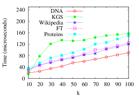
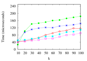
Figure 1: Time performance as a function of $k$, for $m=3$ (left) and $m=8$ (right).

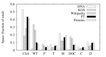
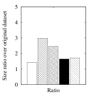
Figure 2: Space consumption of the different compact data structures employed (left) and the size ratio over the original dataset for the different collections (right).

Figure 1 shows time performance as a function of $k$. The time taken by the CSA search is always near 20 microseconds, after which the index takes about $k$ microseconds. In some cases (KGS, or Wikipedia for $m=8$) there are no enough results with frequency larger than 1, and document listing must be activated, which slows down the process to $1.6k$–$4k$ microseconds. Note that in practice one may wish to avoid listing those low-frequency documents anyway.

Figure 2 (left) shows the fraction of space used by the different data structures employed: the CSA, the augmented wavelet tree (WT), the DAC-encoded frequencies (F), the suffix tree topology (T), the document identifiers (DOC), the mapping bitmaps $B$ and $L$ (M), the RMQ structure for Muthukrishnan’s document listing (C), and the sparse bitmap $D$ marking document limits. Figure 2 (right), shows the size ratio over the original dataset (considering one byte per symbol). The values vary between 1.5 and 3 times the size of the collection. Note that, within this space, we can reproduce any document of the collection, as our CSA offers access to them.

6 Final Remarks

	vs compressed [22]				vs uncompressed [22]
Collection	$\times$ space	speedup			$\times$ space	speedup
		$m$	$k=10$	$k=100$		$m$	$k=10$	$k=100$
KGS	0.90	3	13.6	13.0	0.85	3	3.9	5.8
		8	24.3	26.1		8	3.1	5.3
Wikipedia	1.05	3	4.2	4.4	0.79	3	2.5	1.0
		8	6.4	5.9		8	3.4	3.6
Proteins	0.53	3	2.8	1.1	0.41	3	22.0	12.3
		8	28.3	2.2		8	2.0	0.8

Table 1: Comparison to the best previous work [22], giving the fraction of their space we use, and the speedup we obtain with respect to them.

Table 1 compares our solution with previous work [22] on the three collections shared, taking their best compressed (from their variant WT-Alpha+SSGST plus more recent improvements) and uncompressed (from their variant WT-Plain+SSGST) results. Our structure is at most only 5% larger. When both use about the same space, our structure is 4 to 25 times faster. In other cases our structure can use up to half the space, and it is still faster, up to 3 times (for large $k$ and $m$ we must resort to much document listing, where their wavelet tree on documents is faster).

Needless to say, this is a remarkable result for a structure that, in theory [20], used about 80 times the collection size. We have sharply compressed it while retaining the best ideas that led to its optimal time. We believe this establishes a new direction in which research on space-efficient top-$k$ retrieval could be focused: Rather than sampling the suffix tree nodes [12, 22], threshold the document frequencies we store (curiously, this is closer in spirit to the first, superlinear-size, proposed top-$k$ solution [13, 10]). For example, can we discard all the frequencies below a threshold $f$ and efficiently list them if needed? Our work shows this is possible at least for $f=1$.

Our approach easily extends to relevance functions other than term frequency. In most cases it is sufficient to store the appropriate weights in our data structure. Even if these are not compressible, the space should not grow up too much. Our structure also trivially solves other document listing problems, like $k$-mining (list the documents where $P$ appears at least $k$ times). Muthukrishnan [18] solves it in optimal time $O(m+occ)$ and $O(n\log n)$ bits for $k$ fixed at indexing time. For variable $k$ the space is $O(n\log^{2}n)$. Our compressed structure, without modifications, solves both variants in time $O(m+(occ+\log\log n)\log\log n)$.

References

- [1]
- [2] D. Arroyuelo, R. Cánovas, G. Navarro, and K. Sadakane. Succinct trees in practice. In Proc. 11th ALENEX, pages 84–97, 2010.
- [3] D. Belazzougui and G. Navarro. Alphabet-independent compressed text indexing. In Proc. 19th ESA, pages 748–759, 2011.
- [4] D. Belazzougui and G. Navarro. Improved compressed indexes for full-text document retrieval. In Proc. 18th SPIRE, pages 386–397, 2011.
- [5] N. R. Brisaboa, S. Ladra, and G. Navarro. Directly addressable variable-length codes. In Proc. 16th SPIRE, pages 122–130, 2009.
- [6] F. Claude and G. Navarro. Practical rank/select queries over arbitrary sequences. In Proc. 15th SPIRE, pages 176–187, 2008.
- [7] J. Fischer and V. Heun. Space-efficient preprocessing schemes for range minimum queries on static arrays. SIAM J. Comput., 40(2):465–492, 2011.
- [8] R. González, Sz. Grabowski, V. Mäkinen, and G. Navarro. Practical implementation of rank and select queries. In Proc. Posters 4th WEA, pages 27–38, 2005.
- [9] R. Grossi, A. Gupta, and J. Vitter. High-order entropy-compressed text indexes. In Proc. 14th SODA, pages 841–850, 2003.
- [10] W.-K. Hon, M. Patil, R. Shah, and S.-B. Wu. Efficient index for retrieving top-k most frequent documents. J. Discr. Alg., 8(4):402–417, 2010.
- [11] W.-K. Hon, R. Shah, and S. Thankachan. Towards an optimal space-and-query-time index for top- document retrieval. In Proc. 23rd CPM, pages 173–184, 2012.
- [12] W.-K. Hon, R. Shah, and J. S. Vitter. Space-efficient framework for top-k string retrieval problems. In Proc. 50th FOCS, pages 713–722, 2009.
- [13] W.-K. Hon, R. Shah, and S.-B. Wu. Efficient index for retrieving top- most frequent documents. In Proc. 16th SPIRE, pages 182–193, 2009.
- [14] V. Mäkinen and G. Navarro. Position-restricted substring searching. In Proc. 7th LATIN, pages 703–714, 2006.
- [15] U. Manber and E. W. Myers. Suffix arrays: A new method for on-line string searches. SIAM J. Comput., 22(5):935–948, 1993.
- [16] G. Manzini. An analysis of the Burrows-Wheeler transform. J. ACM, 48(3):407–430, 2001.
- [17] I. Munro. Tables. In Proc. 16th FSTTCS, pages 37–42, 1996.
- [18] S. Muthukrishnan. Efficient algorithms for document retrieval problems. In Proc. 13th SODA, pages 657–666, 2002.
- [19] G. Navarro and V. Mäkinen. Compressed full-text indexes. ACM Comp. Surv., 39(1):article 2, 2007.
- [20] G. Navarro and Y. Nekrich. Top-k document retrieval in optimal time and linear space. In Proc. 23rd SODA, pages 1066–1077, 2012.
- [21] G. Navarro and L. Russo. Space-efficient data-analysis queries on grids. In Proc. 22nd ISAAC, pages 323–332, 2011.
- [22] G. Navarro and D. Valenzuela. Space-efficient top-k document retrieval. In Proc. 11th SEA, pages 307–319, 2012.
- [23] D. Okanohara and K. Sadakane. Practical entropy-compressed rank/select dictionary. In Proc. 8th ALENEX, 2007.
- [24] C. Clarke S. Büttcher and G. Cormack. Information Retrieval: Implementing and Evaluating Search Engines. MIT Press, 2010.
- [25] S. Puglisi S. Culpepper, G. Navarro and A. Turpin. Top-k ranked document search in general text databases. In Proc. 18th ESA, pages 194–205, 2010.
- [26] K. Sadakane and G. Navarro. Fully-functional succinct trees. In Proc. 21st SODA, pages 134–149, 2010.
- [27] W. Szpankowski. A generalized suffix tree and its (un)expected asymptotic behaviors. SIAM J. Comput., 22(6):1176–1198, 1993.
- [28] P. Weiner. Linear pattern matching algorithms. In Proc. Switching and Automata Theory, pages 1–11, 1973.
- [29] D. E. Willard. Log-logarithmic worst case range queries are possible in space . Inf. Proc. Lett., 17:81–84, 1983.