Dissipative and stochastic geometric phase of a qubit within a canonical Langevin framework

Abstract

Dissipative and stochastic effects in the geometric phase of a qubit are taken into account using a geometrical description of the corresponding open–system dynamics within a canonical Langevin framework based on a Caldeira–Leggett like Hamiltonian. By extending the Hopf fibration $S^{3}\to S^{2}$ to include such effects, the exact geometric phase for a dissipative qubit is obtained, whereas numerical calculations are used to include finite temperature effects on it.

Introduction. The concept of geometric phase (GP) in quantum systems was proposed by Berry Berry1984 when he studied the dynamics of an isolated quantum system that undergoes an adiabatic cyclic evolution. This cyclic evolution is due to the variation of parameters of the Hamiltonian and is accompanied by a change of the wavefunction by an additional phase factor which depends only on the geometric structure of the space of parameters. The underlying mathematical structure behind GPs was pointed out almost simultaneously by Simon Simon1983 . Soon after, the generalization to non–adiabatic cyclic evolution was carried out by Aharonov and Anandan Aharonov1987 and non-cyclic evolution and sequential projection measurements by Samuel and Bhandary Samuel1988 . Although GPs have been observed in the laboratory Tomita1986 ; Bitter1987 ; Leek2007 , realistic quantum systems are always subject to decoherence due to their surroundings. Therefore, the extension of the GP to the case of open quantum systems becomes fundamental. The first formal extension of the GP was carried out by introducing the concept of parallel transport along density operators Uhlmann1986 . In a more physical context, the concept of GP was generalized for non–degenerated mixed states Sjoqvist2000 and for degenerate mixed–states under unitary evolution Carollo2003 . Using a kinematic approach Mukunda1993 , GPs for mixed states in non–unitary evolution were addressed Tong2004 . Within a spin–boson model, GPs in open quantum systems have also been calculated Whitney2004a together with a study of their geometric nature Whitney2004b . A different approach was introduced in Ref. Marzlin2004 , where the GP was described by a distribution. In classical physics, the counterpart of the Aharonov–Anandan (or Berry) phase was early discovered by Hannay Hannay1985 . Regarding classical dissipative systems, GP shifts have been defined in dissipative limit cycle evolution Kepler1991 ; Ning1992 ; Landsberg1992 , showing that they can be identified with the classical Hannay angle in an extended phase space Sinitsyn2008 . Moreover, GPs can be constructed for a purely classical adiabatically slowly driven stochastic dynamics Sinitsyn2007a ; Sinitsyn2007b ; Sinitsyn2009 .

In this Letter we tackle the problem of including dissipative and stochastic effects in the GP of a qubit. Our study will be based on a geometrical description for a non–isolated qubit within a canonical Langevin framework (see Dorta2012 and references therein) using a Caldeira–Leggett like Hamiltonian Leggett1987 .

Mathematical preliminaries. It is well known that if $|\Psi\rangle$ represents a normalized $n$–level system, then $|\Psi\rangle\in S^{2n-1}$. Thus, the geometry of odd–dimensional spheres is related to the quantum mechanics of finite–dimensional Hilbert spaces. In fact, the celebrated Hopf fibration Hopf1931 relates the quantum and classical description of qubits by means of the map $\pi:S^{3}\to S^{2}$. This map can be understood as a composition, $\pi=\Xi\circ\Omega$, where $\Omega:S^{3}\subset\mathbb{C}^{2}\to\mathbb{C}P^{1}$ sends an element of $\mathbb{C}^{2}$ to its equivalence class and $\Xi:\mathbb{C}P^{1}\left(=\mathbb{C}\cup\infty\right)\to S^{2}$ is given by the stereographic projection. It can be shown that the Hopf map can be written in terms of the Pauli matrices as $\pi\left(|\Psi\rangle\in S^{3}\right)=\left(\langle\Psi|\hat{\sigma}_{x}|\Psi\rangle,\langle\Psi|\hat{\sigma}_{y}|\Psi\rangle,\langle\Psi|\hat{\sigma}_{z}|\Psi\rangle\right)\in S^{2}$, where $\langle\Psi|\hat{\sigma}_{x}|\Psi\rangle^{2}+\langle\Psi|\hat{\sigma}_{y}|\Psi\rangle^{2}+\langle\Psi|\hat{\sigma}_{z}|\Psi\rangle^{2}=1$. Thus, from the Hopf map it can be shown that quantum and classical mechanics may be embedded in the same formulation. Specifically, for a qubit, the Strocchi map Strocchi1966 is exactly the Hopf map previously described. However, the $S^{7}\to S^{4}$ Hopf map, which is an entanglement–sensitive fibration, does not have a classical analog Bentssonbook . As there is a map $S^{2n-1}\to\mathbb{C}P^{n-1}$ and the complex projective space has a natural symplectic structure ($\mathbb{C}P^{n-1}$ is a Kähler manifold), $n$–state systems have a well-defined classical correspondence, which is given by the Strocchi map Strocchi1966 . Thus, one can derive a classical Hamiltonian function for a $n$–level system by defining, for example, appropriate $n$ action–angle coordinates in $\mathbb{C}P^{n-1}$ Oh1994 . For example, as shown in Chruszinskybook , the symplectic structure of $S^{2}$ is responsible for the Aharonov–Anandan GP.

Using the pair of action–angle coordinates $(I,\Phi)$ on $S^{2}$, the Hopf map can be expressed as $\pi\left(|\Psi\rangle\right)=\left(\sqrt{1-I^{2}}\cos\Phi,\sqrt{1-I^{2}}\sin\Phi,I\right)$, where $|\Psi\rangle=a_{1}|1\rangle+a_{2}|2\rangle$ ($a_{j}=|a_{j}|e^{i\phi_{j}}\in\mathbb{C}$), $I\equiv|a_{1}|^{2}-|a_{2}|^{2}$ and $\Phi\equiv\phi_{1}-\phi_{2}$. Thus, the Hamiltonian operator $\hat{H}=\sum_{i}\eta_{i}\hat{\sigma}_{i}$, where $\hat{\sigma}_{i}$ are the Pauli matrices and $\eta_{i}\in\mathbb{R}$, can be Hopf–mapped to a Hamiltonian function, $H_{0}$, given by $H_{0}=-2\sqrt{1-I^{2}}\left(\eta_{1}\cos\Phi+\eta_{2}\sin\Phi\right)+2\eta_{3}I$ (this is the Meyer–Miller-Stock-Thoss Hamiltonian Meyer1979 ; Stock1997 , widely used in molecular physics).

Dissipative–stochastic Hopf fibration of $S^{3}$. Our study will be based on a Caldeira–Leggett Leggett1987 like Hamiltonian for a qubit in the Langevin framework (see Dorta2012 and references therein), which can be expressed as

$$H=H_{0}+\frac{1}{2}\sum_{i}\left(p^{2}_{i}+x^{2}_{i}\omega_{i}^{2}\right)-\Phi\sum_{i}c_{i}x_{i}+\sum_{i}\Phi^{2}c^{2}_{i}$$ (1)

where the oscillator mass has been taken to be one and $c_{i}$ are the system–bath coupling constants. This model takes into account a renormalization term due to the interaction with the environment.

Let us start with pure and normalized quantum states. Using the $(I,\Phi)$ action–angle coordinates, it is easy to see that the unit-radius sphere $S^{2}$ is the set of points satisfying $\left(-\sqrt{1-I^{2}}\cos\Phi\right)^{2}+\left(-\sqrt{1-I^{2}}\sin\Phi\right)^{2}+I^{2}=\nolinebreak 1$. The radius of this sphere remains constant along the time due to energy conservation. That is, the corresponding Hamiltonian function, given by $H_{0}=-\sqrt{1-I^{2}}\left(\cos\Phi+\sin\Phi\right)+I$ remains constant in time (we have taken $\eta_{i}=1$ for simplicity). When Ohmic dissipation is assumed, and after removing the bath variables, the corresponding equations of motion issued from Eq. (1) are

$$\dot{I} = -\sqrt{1-I^{2}}(\sin\Phi+\cos\Phi)-2\gamma\,\dot{\Phi}(t)+\xi(t)$$

$$\dot{\Phi} = \frac{I}{\sqrt{1-I^{2}}}(\cos\Phi+\sin\Phi)+1,$$ (2)

which correspond to the following effective Hamiltonian function $H(t)=-\sqrt{1-I^{2}}\left(\cos\Phi+\sin\Phi\right)+I+2\gamma\Phi\dot{\Phi}-\xi(t)\Phi$. This stochastic dynamics can be interpreted in terms of a stochastic Bloch sphere $S^{2}(\gamma,\xi)$ defined by

$$\left(\sqrt{1-I^{2}}\cos\Phi\right)^{2}+\left(\sqrt{1-I^{2}}\sin\Phi\right)^{2}+I^{2}=1-\gamma\frac{d}{dt}(\Phi^{2})+\xi(t)\Phi,$$ (3)

where $\gamma$ is the friction constant, $\xi(t)$ is a stochastic Gaussian process. The time–dependent radius is given by $R_{t}^{2}(\gamma,\xi)=1-\gamma\frac{d}{dt}(\Phi^{2})+\xi\Phi$. Thus, dissipative and stochastic effects make the Bloch sphere breathe, Eq. (3), by changing its radius in time. This radius is bounded for $\xi=0$, $R_{t}(\gamma,0)\leq 1$. The equality is reached at $t=0$ and at asymptotic times, where thermal equilibrium is reached (in this case, a point in the unit radius sphere represents a pure state). Otherwise, mixed states are represented at each instant of time as points in different spheres of variable radius, as shown in Fig. (1).

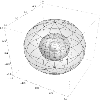
Figure 1: Representation of the dissipative–induced time dependence of the Bloch sphere for $\xi=0$. Time is running in the radial direction.

When $\xi\neq 0$, the square radius becomes a stochastic variable which could reach $R_{t}(\gamma,\xi)\geq 1$ for a particular phase–space trajectory.

The breathing of the Bloch sphere can be geometrized by extending its round metric by adding both dissipation and noise. If these terms are included, the metric of $S^{2}(\gamma,\xi)$ can be written as $ds^{2}\left[S^{2}(\gamma,\xi)\right]=R_{t}^{2}(\gamma,\xi)ds^{2}\left[S^{2}\right]$, where $ds^{2}\left[S^{2}\right]=\frac{dI^{2}}{1-I^{2}}+(1-I^{2})d\Phi^{2}$ is the round–metric for $S^{2}$ in action–angle coordinates.

In order to calculate the stochastic GP, let us start with pure states. If we choose an orthonormal moving frame field $\sigma^{1}=\frac{dI}{\sqrt{1-I^{2}}}$, $\sigma^{2}=\sqrt{1-I^{2}}d\Phi$, then $d\sigma^{2}=-\frac{I}{\sqrt{1-I^{2}}}dI\wedge d\Phi=-I\sigma^{1}\wedge d\Phi=Id\Phi\wedge\sigma^{1}$. Using Cartan’s first structure equation, we obtain the only non-vanishing connection one–form, $\omega=Id\Phi$. Thus, the dynamic phase is obtained as $\phi_{d}=\oint\omega=\oint Id\Phi=\pi I=\pi\cos\theta$. If $S^{2}$ is considered as an embedded submanifold of $S^{3}$, taking into account that the spin connection of $S^{3}$ is $\tilde{\omega}=d\Xi+Id\Phi$, where $\Xi$ is the extra Euler angle which parametrizes the third dimension, it can be shown Bentssonbook that $S^{2}$ inherits from $S^{3}$ the connection one–form $\tilde{\omega}=(I-1)d\Phi$. Thus, the GP is expressed as $\phi_{g}=\oint\tilde{\omega}$. Now, if dissipation and noise are taken into account, the orthonormal moving frame field is given by $R_{t}(\gamma,\xi)\sigma^{i}$ with $i=1,2$. In this case, the only non-vanishing connection one–form is $\omega(\gamma,\xi)=R_{t}(\gamma,\xi)Id\Phi=R_{t}(\gamma,\xi)\omega$. This allows us to define the stochastic dynamic phase acquired after a cycle of period $T$ as $\phi_{d}(\gamma,\xi)=\oint\omega(\gamma,\xi)=\oint R_{t}(\gamma,\xi)I(T)d\Phi=\cos\theta(T)\oint\sqrt{1-\gamma\frac{d}{dt}(\Phi^{2})+\xi\Phi}d\Phi$. Therefore, the stochastic connection one–form, which can be defined as $\tilde{\omega}(\gamma,\xi)=\left[IR_{t}(\gamma,\xi)-1\right]d\Phi$, leads to the corresponding GP

$$\phi_{g}(\gamma,\xi)=\oint\tilde{\omega}(\gamma,\xi)=\oint\left[I(T)R_{t}(\gamma,\xi)-1\right]d\Phi=\oint\left(I(T)\sqrt{1-\gamma\frac{d}{dt}(\Phi^{2})+\xi\Phi}-1\right)d\Phi.$$ (4)

Notice that the dynamics driven by this kind of Caldeira–Leggett like coupling could be interpreted in terms of a mapping between conformal spheres with conformal unitary group fibers at each instant. Moreover, the GP defined by Eq. (4) becomes $\tilde{\phi}_{g}(\gamma,\xi)=\oint\left(I\sqrt{1-\gamma\frac{d}{dt}(\tilde{\Phi}^{2})+\xi\tilde{\Phi}}-1\right)d\tilde{\Phi}$ under the transformation $|\tilde{\Psi}\rangle=e^{i\alpha}|\Psi\rangle$ (or $\tilde{\Phi}=\Phi+\alpha$). Thus, $\phi_{g}(\gamma,\xi)$ is a gauge invariant quantity.

Dissipative qubit (zero temperature). Let us consider a simple qubit which can be represented by the Hamiltonian operator $\hat{H}=\epsilon\hat{\sigma}_{z}$. The corresponding dissipative dimensionless Hamiltonian function ($t\rightarrow 2\epsilon t$), which can be written as $H(t)=I+\frac{\gamma}{2\epsilon}\Phi\dot{\Phi}$, leads to the pair of coupled equations $\dot{I}=-\frac{\gamma}{2\epsilon}\dot{\Phi}$ and $\dot{\Phi}=1$ with solutions $I(t)=I_{0}-\frac{\gamma}{2\epsilon}t$ and $\Phi(t)=\Phi_{0}+t$, where $I_{0}$ and $\Phi_{0}$ are the initial conditions of the action–angle variables. After a cycle of period $T=2\pi$ (the scaled Rabi frequency is $\omega_{0}=1$), the dissipative GP can be computed as

$$\phi_{g}(\gamma) = \oint\left[R_{t}(\gamma)I-1\right]d\Phi$$

$$= \oint\left[I(T)\sqrt{1-\frac{\gamma}{2\epsilon}\Phi\dot{\Phi}}-1\right]d\Phi$$

$$= -\pi+\frac{4}{3}\left[\left(1-\frac{\pi\gamma}{2\epsilon}\right)^{3/2}-1\right]\left(\pi-\frac{\epsilon}{\gamma}\cos\theta_{0}\right),$$

where $I_{0}=\cos\theta_{0}$. Notice that the non–dissipative GP is recovered when $\gamma\to 0$.

It is also interesting to remark that Eq. (Dissipative and stochastic geometric phase of a qubit within a canonical Langevin framework) is only valid for $\gamma\pi/2\epsilon\leq 1$, which reflects nothing but the Caldeira–Leggett energy renormalization in an Ohmic environment. Moreover, this energy renormalization can be re–interpreted in terms of a Bloch sphere whose radius developes harmonic oscillations. In order to show this statement in simple terms, let us introduce the damping factor by means of the phenomenological Caldirola–Kanai Hamiltonian Razavi2005 ; Caldirola1941 ; Kanai1948 for a harmonic oscillator (which is equivalent to the corresponding Caldeira–Leggett Hamiltonian for the oscillator at zero temperature). The Hamiltonian reads $H=(1/2)p^{2}e^{-\frac{\gamma}{2\epsilon}\pi t}+q^{2}e^{\frac{\gamma}{2\epsilon}\pi t}$ (the $\pi$ factor has been introduced to note that time evolution is cyclic). It is straightforward to derive the corresponding equations of motion, leading to $\ddot{y}+\left[1-\left(\frac{\gamma\pi}{2\epsilon}\right)^{2}\right]y=0$, where $y=p,q$. Thus, the renormalized frequency due to the damping term is $\bar{\omega}^{2}=\omega_{0}^{2}-\left(\frac{\gamma\pi}{2\epsilon}\right)^{2}$ which has physical sense only when $\gamma\pi/2\epsilon\leq 1$, as Eq. (Dissipative and stochastic geometric phase of a qubit within a canonical Langevin framework) shows. Therefore, the radius of the Bloch sphere developes harmonic oscillations with a renormalized frequency (another interpretation is that $|I(t)|\leq 1$ requires $\gamma\pi/2\epsilon\leq 1$).

The weak coupling limit of the GP given by Eq. (Dissipative and stochastic geometric phase of a qubit within a canonical Langevin framework) can be expressed as

$$\phi_{g}(\gamma)=-\pi\left(1-\cos\theta_{0}\right)-\frac{\gamma}{\epsilon}\left(\frac{\pi}{2}\right)^{2}\left(\cos\theta_{0}+4\right)+\mathcal{O}(\gamma^{2}).$$ (6)

A direct comparison with other authors Carollo2003 ; Tong2004 ; Marzlin2004 is not pertinent since different models of dissipation and other approaches to calculate the GP were used.

On the other hand, for this dissipative dynamics, information on interference experiments can be straightforwardly extracted from the probability density itself. The typical interference intensity, $J_{t}$, evolves in time according to $J_{t}\propto|\Psi(t)|^{2}\propto 1+\sqrt{1-I^{2}(t)}\cos\Phi(t)=1+\sqrt{1-\left(I_{0}-\frac{\gamma}{2\epsilon}t\right)^{2}}\cos(t+\Phi_{0})$, depending critically on the ratio $\gamma/2\epsilon$ which is directly related to the GP given by Eq. (Dissipative and stochastic geometric phase of a qubit within a canonical Langevin framework).

Stochastic qubit (non–zero temperature). Noise effects can be included in a simple way by assuming a Gaussian stochastic process with distribution function $\rho(\xi;\beta)=\sqrt{\frac{\beta}{2\pi}}\exp{\left(-\frac{\beta\xi^{2}}{2}\right)}$, where $\beta$ is the inverse of the temperature, which is given in units of $2\epsilon$. Thus, for a qubit, the squared radius is also a stochastic process given by $R_{t}^{2}(\gamma,\xi)=1+(\xi-\frac{\gamma}{2\epsilon})\Phi$. Therefore, the stochastic GP acquired after a cycle of period $T$ is given by

$$\phi_{g}(\gamma;\beta)=\left(\cos\theta(T)-\frac{\gamma\pi}{2\epsilon}\right)\left[\oint\int_{-\infty}^{\infty}\sqrt{1-\Phi\left(\frac{\gamma}{2\epsilon}-\xi\right)}\sqrt{\frac{\beta}{2\pi}}\exp{\left(-\frac{\beta\xi^{2}}{2}\right)}d\xi d\phi\right]-\pi.$$ (7)

The previous integral in the noise variable has no analytic solution. Thus, we firstly integrate in $\Phi$ obtaining

$$\phi_{g}(\gamma;\beta)=\left(\cos\theta(T)-\frac{\gamma\pi}{2\epsilon}\right)\left[\int_{-\infty}^{\infty}-\frac{2}{3}\left(\frac{\gamma}{2\epsilon}-\xi\right)^{-1}\left[\left(1-\bigl{\{}\frac{\gamma}{2\epsilon}-\xi\bigl{\}}\pi\right)^{3/2}-1\right]\sqrt{\frac{\beta}{2\pi}}\exp{\left(-\frac{\beta\xi^{2}}{2}\right)}d\xi\right]-\pi.$$ (8)

To illustrate the computation of this integral (which does not have any analytical solution either), only the GP for a non–dissipative qubit at finite temperature will be considered. Moreover, as the noise term becomes more important for high temperatures, we assume that the mean of the Gaussian process is $\beta^{-1}$. Therefore, the GP can be factorized as

$$\phi_{g}(\beta)=\cos\theta_{0}\left[\int_{-\infty}^{\infty}\frac{2}{3\xi}\left[\left(1+\xi\pi\right)^{3/2}-1\right]\sqrt{\frac{\beta}{2\pi}}\exp{\bigl{\{}-\frac{\beta(\xi-\beta^{-1})^{2}}{2}\bigl{\}}}d\xi\right]-\pi\equiv\cos\theta_{0}f(\beta)-\pi,$$ (9)

where $f(\beta)$ encodes the thermal information of the GP acquired by an isolated qubit. This function is depicted in Fig. (2) within a large range of temperatures, displaying a linear behavior at high temperatures and a crossover at a critical temperature given by $T_{c}\approx 2\epsilon$ ($T_{c}\approx 1$ if adimensional temperatures are used). This temperature corresponds to the energy difference of the two levels of the qubit. Moreover, as $f(\beta)\to\pi$ at very low temperatures, the GP acquired for the pure state at zero temperature is recovered. Finally, notice that this type of calculations can be straightforwardly extended to any dissipation value.

Figure 2: Thermal behavior of the GP obtained by numerical integration of Eq. (9) (double logarithmic scale is used). Notice that $f(\beta)\to\pi$ at very low temperatures.

In summary, a geometrical description of the dissipative and stochastic dynamics of a qubit within a Langevin formalism (with a Caldeira–Leggett like coupling) has been developed. The Hopf fibration $S^{3}\to S^{2}$ has been extended to include both stochastic and dissipative effects in terms of a Bloch sphere which develops harmonic oscillations (in the dissipative case). This procedure has allowed us to define a gauge invariant geometric phase, which has been computed for both dissipative and stochastic cases.

This work has been funded by the MICINN (Spain) through Grant Nos. CTQ2008–02578 and FIS2011–29596-C02-01. P. B. acknowledges a Juan de la Cierva fellowship from the MICINN.

References

- (1) M. V. Berry, Proc. R. Soc. London A 329, 45 (1984).
- (2) B. Simon, Phys. Rev. Lett. 51, 2167 (1983).
- (3) Y. Aharonov and J. Anandan, Phys. Rev. Lett. 58, 1593 (1987).
- (4) J. Samuel and R. Bhandari, Phys. Rev. Lett. 60, 2339 (1988).
- (5) A. Tomita and R. Y. Chiao, Phys. Rev. Lett. 57, 937 (1986).
- (6) T. Bitter and D. Dubbers, Phys. Rev. Lett. 59, 251 (1987).
- (7) P. J. Leek et al., Science 318, 1889 (2007).
- (8) A. Uhlmann, Rep. Math. Phys. 24, 229 (1986).
- (9) E. Sjöqvist et al., Phys. Rev. Lett. 85, 2845 (2000).
- (10) A. Carollo, I. Fuentes–Guridi, M. F. Santos and V. Vedral, Phys. Rev. Lett. 90, 160402 (2003).
- (11) N. Mukunda and B. Simon, Ann. Phys. (N. Y.) 228, 205 (1993).
- (12) D. M. Tong, E. Sjoqvist, L. C. Kwek and C. H. Oh, Phys. Rev. Lett. 93, 080405 (2004).
- (13) R. S. Whitney and Y. Gefen, Phys. Rev. Lett. 90, 190402 (2003).
- (14) R. S. Whitney, Y. Makhlin, A. Shnirman and Y. Gefen, Phys. Rev. Lett. 94, 070407 (2005).
- (15) K. -P. Marzlin, S. Ghose and B. C. Sanders, Phys. Rev. Lett. 93, 260402 (2004).
- (16) J. H. Hannay, J. Phys. A: Math. Gen. 18, 221 (1985).
- (17) T. B. Kepler and M. L. Kagan, Phys. Rev. Lett., 66, 847 (1991).
- (18) C. Z. Ning and H. Haken, Phys. Rev. Lett., 68, 2109 (1992).
- (19) A. S. Landsberg, Phys. Rev. Lett., 69, 865 (1992).
- (20) N. A. Sinitsyn and J. Ohkubo, J. Phys. A: Math. Theor. 41, 262002 (2008).
- (21) N. A. Sinitsyn and I. Nemenman, Europhys. Lett. 77, 58001 (2007)
- (22) N. A. Sinitsyn and I. Nemenman, Phys. Rev. Lett., 99, 220408 (2007).
- (23) N. A. Sinitsynm, J. Phys. A: Math. Theor. 42, 193001 (2009).
- (24) A. Dorta–Urra et al., J. Chem. Phys. 136, 174505 (2012).
- (25) A. J. Legget et al., Rev. Mod. Phys. 59, 1 (1987).
- (26) H. Hopf, Matematische Annalen 104, 637 (1931).
- (27) F. Strocchi, Rev. Mod. Phys. 38, 36 (1966).
- (28) I. Bengtsson and K. Zyczkowski Geometry of Quantum States: An Introduction to Quantum Entanglement, Cambridge University Press, Cambridge, UK (2006).
- (29) P. Oh and M. H. Kim, Mod. Phys. Lett A 9, 3334 (1994).
- (30) D. Chruszinsky and A. Jamiolkovsky, Geometric Phases in Classical and Quantum Mechanics, Progress in Mathematical Physics 36, Birkhäuser, Boston (2004).
- (31) H.-D. Meyer and W. H. Miller, J. Chem. Phys. 70, 3214 (1979).
- (32) G. Stock and M. Thoss, Phys. Rev. Lett. 78, 578 (1997).
- (33) M. Razavi, Classical and Quantum Dissipative Systems, Imperial College Press, London (2005)
- (34) P. Caldirola, Nuovo Cimento 18, 393 (1941).
- (35) E. Kanai, Progr. Theor. Phys. 3, 440 (1948).