Testing whether jumps have finite or infinite activity
Abstract
We propose statistical tests to discriminate between the finite and infinite activity of jumps in a semimartingale discretely observed at high frequency. The two statistics allow for a symmetric treatment of the problem: we can either take the null hypothesis to be finite activity, or infinite activity. When implemented on high-frequency stock returns, both tests point toward the presence of infinite-activity jumps in the data.
doi:
10.1214/11-AOS873keywords:
[class=AMS] .keywords:
.and a1Supported in part by NSF Grants DMS-05-32370 and SES-0850533.
1 Introduction
Traditionally, models with jumps in finance have relied on Poisson processes, as in Merton (1976), Ball and Torous (1983) and Bates (1991). These jump-diffusion models allow for a finite number of jumps in a finite time interval, with the idea that the Brownian-driven diffusive part of the model captures normal asset price variations while the Poisson-driven jump part of the model captures large market moves in response to unexpected information. More recently, financial models have been proposed that allow for infinitely many jumps in finite time intervals, using a variety of specifications, such as the variance gamma model of Madan and Seneta (1990) and Madan, Carr and Chang (1998), the hyperbolic model of Eberlein and Keller (1995), the CGMY model of Carr et al. (2002) and the finite moment log stable process of Carr and Wu (2003a). These models can capture both small and frequent jumps, as well as large and infrequent ones.
In this paper, we develop statistical procedures to discriminate empirically between the two situations of finite and infinite number of jumps, while allowing in both cases for the presence of a continuous component in the model. While many theoretical models make use of one or the other type of jumps, no statistical test has been proposed so far that can identify the most likely type in a given data set, as existing tests have focused on the issue of testing for the presence of jumps but not distinguishing between different types of jumps; see Aït-Sahalia (2002), Carr and Wu (2003b), Barndorff-Nielsen and Shephard (2004), Huang and Tauchen (2005), Andersen, Bollerslev and Diebold (2007), Jiang and Oomen (2008), Lee and Mykland (2008), Aït-Sahalia and Jacod (2009b) and Lee and Hannig (2010), among others.
The setup we consider is one where a univariate process is observed on a fixed time interval , at discretely and regularly spaced times . In a typical high-frequency financial application, will be the log of an asset price, the length of observation ranges from, say, one day to one year, while the sampling interval is small, typically measured in seconds. Assuming that the observed path has jumps, we want to test whether there are a finite number of jumps or not on that path, two properties commonly referred to as “finite activity” or “infinite activity” for the jump component of .
Our aim is to provide asymptotic testing procedures, as the time lag between successive observations goes to , allowing to decide which of these two hypotheses is more likely; that is, we want to decide in which of the two complementary subsets
of the sample space we are in.
More specifically, we want to find tests with a prescribed asymptotic significance level, and with asymptotic power going to , to test the null hypothesis that is in , and also the symmetric null hypothesis that the observed is in . We will need some assumptions on the process , basically that it is an Itô semimartingale. However, we wish to keep the solution as nonparametric as possible, and in particular we do not want to specify the structure of the volatility or of the jumps.
The simple idea behind the two test statistics we propose is common with our earlier work on testing whether jumps are present or not, or whether a continuous component is present. We compute certain power variations of the increments, suitably truncated and/or sampled at different frequencies. Related methodologies are being utilized by other authors. For example, Todorov and Tauchen (2010) use the test statistics of Aït-Sahalia and Jacod (2009b), study its logarithm for different values of the power argument and contrast the behavior of the plot above two and below two in order to identify the presence of a Brownian component. Cont and Mancini (2009) use threshold or truncation-based estimators of the continuous component of the quadratic variation, originally proposed in Mancini (2001), in order to test for the presence of a continuous component in the price process. The resulting test is applicable when the jump component of the process has finite variation, and a test for whether the jump component indeed has finite variation is also proposed. In terms of the Blumenthal–Getoor index , this corresponds to testing whether .
We aim here to construct test statistics which are simple to compute and have the desirable property of being model-free. In particular, no feature of the dynamics of the underlying asset price, which can be quite complex with potentially jumps of various activity levels, stochastic volatility, jumps in volatility, etc., need to be estimated in order to compute either the statistic or its distribution under the null hypothesis. In fact, implementing the two tests we propose requires nothing more than the computation of various truncated power truncations.
We consider two testing problems, one where the null hypothesis is finite jump activity and its “dual” where the null hypothesis is infinite jump activity. Under the null hypothesis of finite-activity jumps, the test statistic we propose is similar to the simpler statistic of Aït-Sahalia and Jacod (2009b) which was employed to test for the presence of jumps, with an additional truncation step. An appropriately selected truncation mechanism eliminates finite-activity jumps, so that the probability limit of the statistic post-truncation is the same in this paper as that of the simpler statistic in the earlier work, under a purely continuous model. While the result is indeed in that case that “the answer is the same,” this is not completely obvious a priori and still needs to be established mathematically. And the commonality is limited to probability limits: the two statistics have different asymptotic distributions.
Under the reverse scenario, where the null hypothesis is that jumps are infinitely active, then the statistic we propose for this purpose is radically new and so is its asymptotic behavior. That second statistic has no relationship to previous work.
As we will see below, when implemented on high-frequency stock returns, both tests point toward the presence of infinitely active jumps in the data. That is, in the test where is the null hypothesis, we reject the null; in the test where is the null hypothesis, we fail to reject the null. This is in line with the empirical results of a companion paper, Aït-Sahalia and Jacod (2009a), which contains an extension to Itô semimartingales of the classical Blumenthal–Getoor index for Lévy processes and estimators for ; see also Belomestny (2010) for different estimators. This parameter takes values between and and plays the role of a “degree of jump activity” for infinitely active jump processes. Then if the estimator of is found to be “high” in its range , with a confidence interval excluding , as it is the case in the empirical findings of Aït-Sahalia and Jacod (2009a), it is a strong evidence against finite activity. However, finite activity implies , but the converse fails, so using estimators of can at the best allow for tests when the null is “infinite activity,” and even for this it does not allow for determining the asymptotic level of the test. Thus in fact the present paper and the other one are complementary, both aiming to have a picture as complete as possible of a continuous-time process which is discretely observed at increasing frequencies. Finally we can also mention that here the assumptions are significantly weaker than in Aït-Sahalia and Jacod (2009a), in the sense that the test proposed here is nonparametric, where the estimator of proposed there is parametric.
The paper is organized as follows. Section 2 describes our model and the statistical problem. Our testing procedure is described in Section 3, and Sections 4 and 5 are devoted to a simulation study of the tests and an empirical implementation on high-frequency stock returns. Technical results are gathered in the supplemental article [Aït-Sahalia and Jacod (2011)].
2 The model
The underlying process which we observe at discrete times is a one-dimensional process which we specify below. Observe that taking a one-dimensional process is not a restriction in our context since, if it were multidimensional, infinitely many jumps on means that at least one of its components has infinitely many jumps, so the tests below can be performed separately on each of the components. In all the paper the terminal time is fixed. However, it is convenient, and not a restriction, to assume that the process is defined over the whole half-line.
Our structural assumption is that is an Itô semimartingale on some filtered space , which means that its characteristics are absolutely continuous with respect to Lebesgue measure. is the drift, is the quadratic variation of the continuous martingale part, and is the compensator of the jump measure of . In other words, we have
Here and are optional process, and is a transition measure from endowed with the predictable -field into . One may then write as
where is a standard Wiener process. It is also possible to write the last two terms above as integrals with respect to a Poisson measure and its compensator, but we will not need this here.
The cutoff level used to distinguish small and large jumps is arbitrary; any fixed jump size will do. In terms of the definition (2), changing the cutoff level amounts to an adjustment to the drift of the process. Ultimately, the question we are asking about the finite or infinite degree of activity of jumps is a question about the behavior of the compensator near There are always a finite number of big jumps. The question is whether there are a finite or infinite number of small jumps. This is controlled by the behavior of near .
2.1 The basic assumptions
The assumptions we make depend on the null hypothesis we want to test. We start with a very mild (local) boundedness assumption. Recall that a process is pre-locally bounded if for , for a sequence of stopping times increasing to .
Assumption 1
The processes , and and are pre-locally bounded.
In some cases we will need something more about the drift and the volatility .
Assumption 2
The drift process is càdlàg, and the volatility process is an Itô semimartingale satisfying Assumption 1.
Under this assumption we can write as (2), with a Wiener process which may be correlated with . Another (equivalent) way of writing this is
| (4) |
where is a local martingale which is orthogonal to the Brownian motion and has jumps bounded by . Saying that satisfies Assumption 1 implies that the compensator of the process has the form , and the processes and are pre-locally bounded, and the process is càdlàg.
Next, we need conditions on the Lévy measures , which are quite stronger than what is in Assumption 1. We state here a relatively restrictive assumption.
Assumption 3
The Lévy measure is of the form
where, for some pre-locally bounded process : {longlist}[(iii)]
, , and are nonnegative predictable processes satisfying
| (6) |
, and are predictable processes, satisfying for some constant
is a signed measure, whose absolute value satisfies, for some increasing continuous function with and some constant :
Equivalently, one could take identically, provided in (6) is substituted with .
Since is allowed to be a signed measure, (3) does not mean that restricted to , say, has the density ; it simply means that the “leading part” of on a small interval has a density behaving as as , and likewise on the negative side.
In all models with jumps of which we are aware in financial economics, such as those cited in the first paragraph of the Introduction, the Lévy measure has a density around , which behaves like as or (in most cases with and constant). Thus all these models satisfy Assumption 3. For instance, it is satisfied if the discontinuous part of is a stable process of index , with and and , and being constants; in this case the residual measure is the restriction of the Lévy measure to the complement of , and (3) holds for any . When the discontinuous part of is a tempered stable process the assumption is also satisfied with the same processes as above, but now the residual measure is not positive in general, although it again satisfies (3) with any . Gamma and two-sided Gamma processes also satisfy this assumption, take and and , and being constant.
This assumption also accounts for a stable or tempered stable or Gamma process with time-varying intensity, when , and are as above, but are genuine processes. It also accounts for a stable with time-varying index process, as well as for being the sum of a stable or tempered stable process with jump activity index plus another process whose jumps have activity strictly less than . Furthermore, any process of the form satisfies Assumption 3 as soon as does and is locally bounded and predictable. As is easily checked (see Section 1 of the supplemental article [Aït-Sahalia and Jacod (2011)] for a formal proof), under Assumption 3 the set of (1) is (almost surely)
| (9) |
The previous assumption is designed for the test for which the null is “finite activity.” For the symmetric test, the assumption we need is stronger:
Assumption 4
We have Assumption 3 with [a constant in ], and .
The reason we need a stronger assumption under the null of infinite jump activity is that the asymptotic distribution of the test statistic under the null is now driven by the behavior of near whereas in the previous situation where the null has finite jump activity it is the Brownian motion that becomes the driving process for the behavior of the statistic under the null.
Assumptions 3 and 4 have the advantage of being easily interpretable and also easy to check for any concrete model. But as a matter of fact it is possible to substantially weaken them, and we do this in the next subsection. The reader who is satisfied with the degree of generality of Assumption 3 can skip the next subsection and go directly to the description of the tests in Section 3.
2.2 Some weaker assumptions
For a better understanding of what follows, let us first recall the notion of Blumenthal–Getoor index (in short, BG index). There are two distinct notions. First, we have a (random) global BG index over the interval defined by
| (10) |
This is a nondecreasing -valued process. It is not necessarily right-continuous, nor left-continuous, but it is always optional. Second, we have an instantaneous BG index , which is the BG index of the Lévy measure , defined as the following (random) number:
| (11) |
which necessarily belongs to . As a process, is predictable. The symmetrical tail function of (defined for ) satisfies for all and :
In the latter case, does not necessarily converge to when . When as for all , or if , we say that the measure is regular: this is the case when, for example, the function is regularly varying at .
The connections between these two indices are not completely straightforward; they are expressed in the next lemma, where denotes the jump of at time :
Lemma 1
Outside a -null set, we have for all :
| (13) |
Moreover if denotes the Lebesgue measure we have, outside a -null set again,
| (14) |
and this inequality is an equality as soon as for all .
Our general assumption involves two functions with the following properties [ is indeed like in (3)]:
| (15) |
Assumption 5
The global BG index takes its values in , and there are a constant , two functions and as in (15) and pre-locally bounded processes and , such that for all and and -almost all we have
| (16) | |||||
This assumption looks complicated, but it is just a mild local boundedness assumption, which is made even weaker by the fact that we use the global BG index instead of the (perhaps more natural) instantaneous index .
Now we introduce the set which will be the alternative for our first test when the null is “finitely many jumps.” This set has a somewhat complicated description, which goes as follows, and for which we introduce the notation (for ):
| (17) |
Then we set
| (18) | |||
| (19) |
| (20) | |||
| (21) |
We will see in Section 1 of the supplemental article [Aït-Sahalia and Jacod (2011)] that , but equality may fail. In view of Lemma 1, and if the measures are regular [see after (2.2)], the set is equal to , which is also the set where there are infinitely many jumps due to a positive BG index. The interpretation of the set is more delicate: observe that by (14); then saying that amounts to saying that for “enough” values of the variables are not small.
The following is proved there:
As for Assumption 4, it can be weakened as follows:
Assumption 6
We associate with this assumption the following increasing process and set:
| (24) |
where the exponent in stands for “infinite activity for the jumps associated with the part of the Lévy measure having index of jump activity ,” and we have , up to a null set. Again, the set is not necessarily empty.
Assumption 4 obviously implies Assumption 6, with the same and with , and in this case . However, Assumption 6, which is exactly the assumption under which the estimation of the BG index is performed in Aït-Sahalia and Jacod (2009a), does not require the measure to be finite when , so it is weaker than Assumption 4.
3 The two tests
3.1 Defining the hypotheses to be tested
Ideally, we would like to construct tests in the following two situations:
| (25) | |||
In order to derive the asymptotic distributions of the test statistics which we construct below, we need to slightly restrict these testing hypotheses. Besides the sets defined in (18) and (24), we also define two other complementary sets:
| (26) |
That is, is the set on which the continuous martingale part of is not degenerate over , and the exponents in and stand for “the Wiener process is present,” and “no Wiener process is present,” respectively.
We will provide tests for the following assumptions (below we state the assumptions needed for the null to have a test with a given asymptotic level, and those needed for the alternative if we want the test to have asymptotic power equal to ):
| (27) | |||
Note that this lets aside the two sets and in the null hypothesis: in the context of high-frequency data, no semimartingale model where is not empty has been used, to our knowledge. Indeed, on this set the path of over the interval is a pure drift plus finitely many jumps. It also lets aside the set , under Assumptions 1 and 6, which is more annoying. Note that the set contains those for which is continuous on , although we would not test against infinite activity if we did not know beforehand that there were some jumps.
Next, we specify the notion of testing when the null and alternative hypotheses are families of possible outcomes. Suppose now that we want to test the null hypothesis “we are in a subset ” of , against the alternative “we are in a subset ,” with of course . We then construct a critical (rejection) region at stage , that is, when the time lag between observations is . This critical region is itself a subset of , which should depend only on the observed values of the process at stage . We are not really within the framework of standard statistics, since the two hypotheses are themselves random.
We then take the following as our definition of the asymptotic size:
| (28) |
Here is the usual conditional probability knowing , with the convention that it vanishes if . If , then , which is a natural convention since in this case we want to reject the assumption whatever the outcome is. Note that features a form of uniformity over all subsets . As for the asymptotic power, we define it as
| (29) |
Again, this is a number.
Clearly, and as in all tests in high-frequency statistics, at any given stage it is impossible to distinguish between finitely many or infinitely many jumps (or, for that matter, between a continuous and a discontinuous path). So testing such hypotheses can only have an asymptotic meaning, as the mesh goes to . Now, our definition of the asymptotic level is the usual one, apart from the fact that we test a given family of outcomes rather than a given family of laws. For the asymptotic power, it is far from the typical usual statistical understanding. Namely saying that , as will often be the case below, does not mean anything like the infimum of the power over all possible alternatives is ; it is rather a form of consistency on the set of alternatives.
3.2 Truncated power variations
Before stating the results, we introduce some notation, to be used throughout. We introduce the observed increments of as
| (30) |
to be distinguished from the (unobservable) jumps of the process, . In a typical application, is a log-asset price, so is the recorded log-return over units of time.
We take a sequence of positive numbers, which will serve as our thresholds or cutoffs for truncating the increments when necessary, and will go to as the sampling frequency increase. There will be restrictions on the rate of convergence of this sequence, expressed in the form
| (31) |
for some : this condition becomes weaker when increases. Two specific values for , in connection with the power which is used below, are of interest to us:
| (32) |
These quantities increase when increases [on ], and .
Finally, with any we associate the increasing processes
| (33) |
consisting of the sum of the th absolute power of the increments of truncated at level , and sampled at time intervals . These truncated power variations, used in various combinations, will be the key ingredients in the test statistics we construct below.
3.3 The finite-activity null hypothesis
We first set the null hypothesis to be finite activity, that is, , whereas the alternative is .
We choose an integer and a real . We then propose the test statistic, which depends on , , and on the truncation level , and on the time interval , defined as follows:
| (34) |
That is, we compute the truncated power variations at two different frequencies in the numerator and denominator, but otherwise use the same power and truncation level Since is an integer, both truncated power variations can be computed from the same data sample. If the original data consist of log-returns sampled every units of time, then sampling every units of time involves simply retaining every th observation in that same sample.
The first result gives the limiting behavior of the statistic , in terms of convergence in probability:
Theorem 1
As the result shows, the statistic behaves differently depending upon whether the number of jumps is finite or not. Intuitively, if the number of jumps is finite, then at some point along the asymptotics the truncation eliminates them and the residual behavior of the truncated power variation is driven by the continuous part of the semimartingale. More specifically, is of order where is the continuous variation of order and is a constant defined below. It follows from this that the ratio in has the limit given in (35) since the numerator and denominator tend to zero but at different rates.
By setting in the truncation rate, we are effectively retaining all the increments of the continuous part of the semimartingale, and so we indeed obtain the “full” continuous variation after truncation. Note that by contrast, the untruncated power variation converges when to the discontinuous variation of order , namely , and so we would not have been able to distinguish finite or infinite jump activity without truncation, as long as jumps (of any activity) are present.
If the jumps have infinite activity, on the other hand, that is, under the alternative hypothesis, the asymptotic behavior of the truncated power variation is driven by the small jumps, whether the Brownian motion is present or not, and the truncation rate matters. We will see, for example, that, under Assumption 4 or 6, the truncated power variation is of order Since here we are truncating at the same level for the two sampling frequencies and this fact has no consequence on the behavior of the ratio , which tends to as stated by (36) even when Assumption 6 fails.
Theorem 1 implies that for the test at hand an a priori reasonable critical region is , for between and , and in particular if we choose in the interval the asymptotic level and power are, respectively, and if the model satisfies Assumption 5.
For a more refined version of this test, with a prescribed level , we need a central limit theorem associated with the convergence in (35), and a standardized version goes as follows [we use to denote the stable convergence in law; see, e.g., Jacod and Shiryaev (2003) for this notion]:
Theorem 2
Note that to implement this asymptotic distribution in practice, and hence the test, we simply need to compute truncated power variations for various powers (specifically and , in this case) and at two different sampling frequencies ( and ). No other estimation is required. In particular, we do not need to estimate any aspect of the dynamics of the such as its drift or volatility processes or its jump measure. In that sense, the test statistic is nonparametric, or model-free.
We are now ready to exhibit a critical region for testing vs. , or , or (depending on the assumptions), using with a prescribed asymptotic level . Denoting by the -quantile of , that is, where is , we set
| (40) |
More precisely, we can state the level and power of the test under selected alternatives as follows:
3.4 The infinite-activity null hypothesis
In the second case, we assume Assumption 6 (or Assumption 4) and we set the null hypothesis to be infinite activity, that is, (or ), whereas the alternative is . Unfortunately, we cannot simply use the same test statistic we proposed in (34) for this second testing problem. The reason is that, while the distribution of is model-free under the null hypothesis of the first testing problem, it is no longer model-free under the null hypothesis of the second testing problem: its distribution when jumps have infinite activity depends upon the degree of jump activity, While it is possible to estimate consistently [see Aït-Sahalia and Jacod (2009a)], it would be preferable to construct a statistic whose implementation does not require a preliminary estimate of the degree of jump activity.
In order to design a test statistic which is model-free under the null of infinite activity, we choose three reals and and then define a family of test statistics as follows:
| (41) |
In other words, unlike the previous statistic , we now play with different powers and and different levels of truncation and but otherwise sample at the same frequency . Once more, the first result states the limiting behavior of in terms of convergence in probability:
Theorem 4
[(b)]
If the sequence satisfies (31) with some , we have
| (42) |
If the sequence satisfies (31) with some , we have
| (43) |
That is, as was the case in Theorem 1, the test statistic tends to under the alternative and to a value different from under the null. Intuitively, under the alternative of finite jump activity, the behavior of each one of the four truncated power variations in (41) is driven by the continuous part of the semimartingale. The truncation level is such that essentially all the Brownian increments are kept. Then the truncated power variations all tend to zero at rate and , respectively, and by construction the (random) constants of proportionality and cancel out in the ratios, producing the limit given in (43).
If, on the other hand, jumps have infinite activity, then the small jumps are the ones that matter and the truncation level becomes material, producing four terms that all tend to zero but at the different orders and , respectively, resulting in the limit (42). By design, the limit is independent of
A reasonable critical region is with between and , and if is in the interval the asymptotic level and power are, respectively, and . For a test with a prescribed level we again need a standardized central limit theorem associated with the convergence in (42):
Theorem 5
As was the case for in Theorem 2, the asymptotic distribution of under the null is again model-free. While the expression (5) looks complicated, implementing it simply requires the computation of truncated power variations of order , and , and at truncation levels and No other aspects of the dynamics of the process, such as its degree of jump activity , for instance, need to be estimated.
The critical region for testing or vs. using with a prescribed asymptotic level will be
| (46) |
We can state more precisely the level and power of the test as follows:
Theorem 6
Under Assumptions 1 and 4 with (resp., Assumption 6 with ), and if the sequence satisfies (31) with some , the asymptotic level of the critical region defined by (46) for testing the null hypothesis “infinite activity for jumps” (i.e., , resp., , against ) equals . Moreover the asymptotic power of this test is .
Under the null hypothesis the rate of convergence is (contrary to the situation of Theorem 3, where the rate was whatever and were). So, although asymptotically does not explicitly show in the test itself, one should probably take as small as possible (we have no choice as to , of course). That is, one should take as large as possible, which in turn results in choosing as large as possible [recall (32)]. We discuss actual choices in practice in Sections 4 and 5 below.
3.5 Microstructure noise
In practice, the tests presented here need a lot of data to be effective, that is, we need a high sampling frequency. However, in this case, it is well established that the so-called microstructure noise may be a relevant consideration, and in some cases may even dominate at ultra high frequencies. It is outside the scope of this paper to provide a complete analysis of what happens when noise is present, or to contemplate constructing effective testing procedures in the presence of noise. However, as a first step, it may be enlightening to determine at least the limiting behavior (in probability) of our test statistics in the presence of noise since this may help guide the interpretation of the empirical results when the test is implemented in practice.
We start first with pure additive noise, which is the type of noise considered by much of the literature, primarily for reasons of tractability, although it may not account very well for the microstructure noise encountered in practice. It gives, however, an insight on what can happen in the presence of noise. In this situation, at any given observation time we actually observe log-returns perturbed by a noise term in
| (47) |
To avoid intricate statements, we make a few basic, and mild, assumptions on the noise process : those variables are i.i.d., centered, independent of the underlying process, with the following property:
|
(48) |
Note that no moment condition is required, except , because we consider only truncated increments.
We write for the variables introduced in (33) if we replace by , and likewise for and if we do the same substitution in (34) and (41) (those are associated with some integer and some numbers and ). Under the above assumption on the noise, we have the following:
It is remarkable that the assumptions in this theorem are much weaker than in the previous results, as far as is concerned. This is of course because the noise, when present, becomes the prevalent factor. This has the important consequence that the statistics and are no longer able to distinguish between the two hypotheses of finite or infinite activity when noise dominates. When we use we get a limit which differs from both limits in Theorem 1, so when we test for the null hypothesis of finite activity and the empirical value of is close to we can in principle tell that this is due to the noise, whereas if it is close to or to this is probably due to finite activity, or infinite activity. When we use the situation is worse, because noise plus finite activity leads to accept the hypothesis that we have infinite activity whether the jumps have finite or infinite activity.
Alternatively, it might be closer to the reality to model the microstructure noise as a pure rounding noise. There, instead of observing we observe that is, rounded to the nearest multiple of , where is the tick size: typically cent for a decimalized stock, or of a dollar, for bond prices. Let us denote by the variables of (33) when we replace by . Theorems 1 and 4 were based on limit theorems for the truncated power variations . In the rounded case we indeed have something radically different: as soon as , we eliminate all increments, because increments are multiples of . Therefore for all large enough, and of course the ratios (34) and (41) make no sense. It follows that in the case of a rounding noise, the statistics proposed in this paper are totally meaningless. And as a matter of fact, even when the whole (rounded) path of is observed, we cannot decide whether we have finitely many or infinitely many jumps. This means that not only our statistics do not work for this problem, but there cannot exist asymptotically consistent tests for this problem.
Naturally, these two idealized descriptions of microstructure noise do not exhaust the possibilities for modeling the noise. One can, for example, use a mixed model which mixes additive noise and rounding, or more general forms, as in Jacod et al. (2009), for example. At present, however, it is not clear how our statistics theoretically behave in these more general cases, nor how to construct asymptotically consistent tests, nor even if such tests exist at all.
4 Simulation results
We now report simulation results documenting the finite sample performance of the test statistics and in finite samples under their respective null and alternative hypotheses. We calibrate the values to be realistic for a liquid stock trading on the NYSE. We use observation lengths ranging from day, consisting of hours of trading, that is, seconds, to year. The sampling frequencies we consider range from second to minutes. The highest sampling frequencies serve to validate the asymptotic theory contained above, while the lower frequencies serve as proxies for situations where sparse sampling is employed as a means to reduce the adverse impact of market microstructure noise.
The tables and graphs that follow report the results of simulations. In order to validate the asymptotic theory developed above, we start with the highest sampling frequency of second. Below, we will examine the accuracy of the tests as a function of the sampling frequencies ranging from seconds to minutes. The data generating process is the stochastic volatility model with , , , , is a compound Poisson jump process with jumps that are uniformly distributed on and . The jump process is either a -stable process with , that is, a Cauchy process (which has infinite activity, and will be our model under ) or a compound Poisson process (which has finite activity, and will be our model under ). In the infinite-activity case, empirical estimates of reported in Aït-Sahalia and Jacod (2009a) are higher than simulation results using -stable processes with such values are qualitatively similar. In the finite-activity case, the jump size of the compound Poisson process is drawn from a truncated Normal distribution with mean and standard deviation , designed to produce jumps greater in magnitude than . The estimator is implemented with a truncation rate where . In the results, we report the level of truncation indexed by the number of standard deviations of the continuous martingale part of the process, defined in multiples of the long-term volatility parameter That is, is such that
The statistic is implemented with and When , the constants appearing in (39) are
| (50) |
For the second test, is implemented with and the second truncation level related to the first according to that is,
Given the scale parameter [or equivalently in (6), which here is a constant] of the stable process in simulations is calibrated to deliver different various values of the tail probability reported in the tables as low (), medium () and high (). For the Poisson process, it is the value of the arrival rate parameter that is set to generate the desired level of jump tail probability as low (), medium () or high (). In the various simulations’ design, we hold fixed. Therefore the tail probability parameter controls the relative scale of the jump component of the semimartingale relative to its continuous counterpart.
| Finite jump intensity | Test theoretical level | Test empirical level for a degree of truncation | ||||||
|---|---|---|---|---|---|---|---|---|
| Low | ||||||||
| Medium | ||||||||
| High | ||||||||
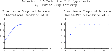
Table 1 reports the Monte Carlo rejection rates of the test of vs. at the and level, using the test statistic for various levels of truncation . Recall that for concreteness is expressed as a number of standard deviations of the Brownian part of . We find that the test behaves well, with empirical test levels close to their theoretical counterparts, and so for a wide range of values of
The limit in probability of is with our choice of and , provided . With our notation denoting the threshold expressed as the number of (normalized) standard deviations of the Brownian part, this means that this limit holds when goes to infinity. In practice we choose between and , and this introduces a bias. To evaluate this bias, in Figure 1, we plot as a function of the limiting value of under when stays fixed instead of increasing to infinity, and compare it with the theoretical limit (in the simple model used for the simulations it is possible to numerically compute it with any desired accuracy); this is the left graph, and on the right graph we draw the corresponding average value of from the Monte Carlo simulations, both as functions of . It is worth noting that the behavior of is driven by that of the Brownian motion component, since the truncation effectively eliminates the finite-activity jumps. For very small values of , , starts below as predicted by the theoretical behavior of the continuous martingale part of Once gets above the theoretical limit of will then remain at as long as is not so large as to start including some jumps.
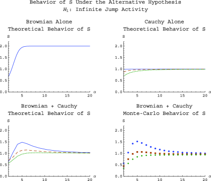
Figure 2 plots the limiting value of (as a function of again) under where the model consists of a Brownian and a Cauchy components as described above. The upper left graph is the theoretical behavior of for the Brownian component taken in isolation, the upper right graph the theoretical behavior for the Cauchy component taken in isolation, the lower left graph the theoretical behavior for the sum of the two components, that is, the model we simulate from, and the lower right graph the corresponding results from the Monte Carlo simulations. When the Cauchy process is present, the three curves in the figure correspond to the low (solid curve), medium (long dashes) and high (short dashes) scale of the jump component relative to the continuous component. For very small values of such as the behavior of tracks that of the Brownian component, which is increasing in toward As increases, the curves then start reversing course and tend to instead, the limit driven by the infinite-activity jump process as shown in (36). The higher the scale of the jump component relative to the continuous component, the more the curve in the lower left graph approximates the corresponding one in the upper right graph, that is, the more it resembles that of a pure Cauchy process. For the Monte Carlo results, the low, medium and high jump scales are represented by circles, squares and diamonds, respectively. In all three cases, they track the predicted theoretical limits closely for each value of the truncation level

=260pt Infinite Test Test jump activity theoretical level empirical level Low Medium High
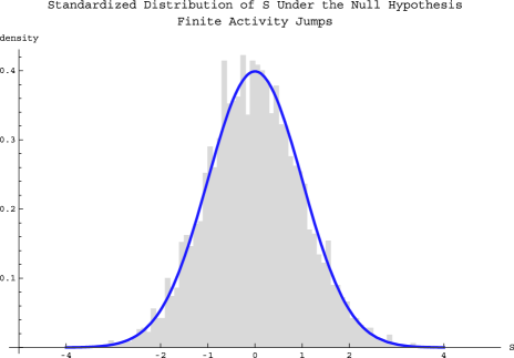
Finally, we report in Figure 3 histograms of the values of the unstandardized computed under , centered in as expected from (35), and centered in as expected from (36), respectively. Figure 4 reports the Monte Carlo distribution of the statistic standardized according to (37), compared to the limiting distribution.
Next, we turn to the symmetric problem, that of testing of vs. which we do using the statistic The results are reported in Table 2 for the test rejection rate under the null hypothesis. Figure 5 shows the limiting value of under as expected from the theoretical limit of given in (42) (lower left graph for the Brownian plus Cauchy model) and the corresponding average value of from the Monte Carlo simulations (lower right graph). The upper graphs in the figure correspond to the Brownian alone (left, with a limit of ) and Cauchy alone (right, with a limit of ) situations. As was the case for the previous test, higher values of the jump scale parameter make the resulting semimartingale model approximate the behavior of its infinite-activity jump component more closely, while for lower scale parameters and low values of the behavior is determined by the continuous component. In all cases, we find that the Monte Carlo results track the predicted theoretical limits for each value of the truncation level Compared to Figure 2, we find that the limit is approached with less precision than was the case of and requires larger values of than was the case for the other test when the infinite-activity jump process is mixed with the continuous component.
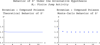
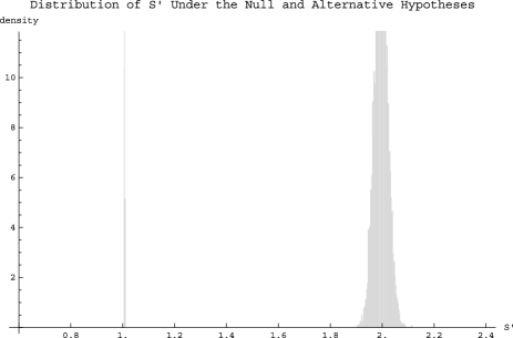
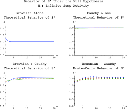
Figure 6 shows the point limit results for under There, the theoretical limit of from (43) is reached quickly, as was the case in Figure 1. This is the case provided that the values of are not so large that jumps start being retained in the calculations. In particular, the value of can become large if is such that a jump is just included at the cutoff but not yet at the cutoff. But in most cases the statistic is very close to when the number of jumps is finite, simply because once is large enough for the truncation level to have eliminated all the jumps at the higher level of truncation then there are very few Brownian increments between truncation levels and ; therefore is only marginally larger than and similarly for power .
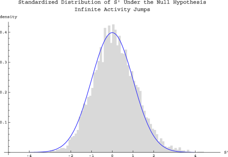
Figure 7 reports the Monte Carlo distributions of under and they are centered at and as expected. Under we note that displays very little variability with the provision above regarding the value of As a general rule, the test based on appears more sensitive to values of than the test based on Figure 8 reports the Monte Carlo and asymptotic distribution of the standardized under according to (44).
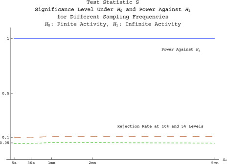
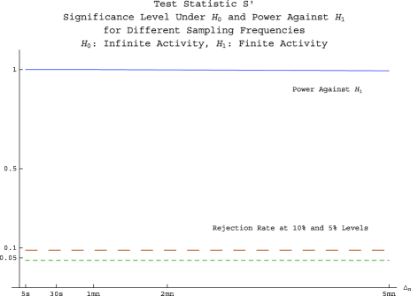
Finally, we examine the accuracy of the tests as a function of the sampling frequencies. We consider for this purpose two experiments. In the first one, we fix the observation length to days (one week) and consider sampling frequencies from seconds to minutes. The sample size therefore decreases by a factor over the range of values of considered. In the second experiment, we consider the same sampling frequencies but increase the length of the observation window from days to year, in order to keep the sample size approximately constant over the range of values of The results of the first experiment are reported in Figures 9 and 10, respectively. We find little size distortion or power loss. The results of the second experiment are, not surprisingly, better and are not shown here in order to save space.
5 Empirical results
In this section, we apply our two test statistics to real data, consisting of all transactions recorded during the year 2006 on two of the most actively traded stocks, Intel (INTC) and Microsoft (MSFT). The data source is the TAQ database. Using the correction variables in the data set, we retain only transactions that are labeled “good trades” by the exchanges: regular trades that were not corrected, changed, or signified as canceled or in error; and original trades which were later corrected, in which case the trade record contains the corrected data for the trade. Beyond that, no further adjustment to the data is made.
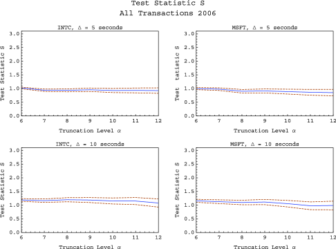
We first consider the test where the null hypothesis consists of finite jump activity. Figure 11 shows the values of the test statistic along with a confidence interval computed from the asymptotic distribution (37) under the finite-activity null hypothesis, plotted for a range of values of the truncation index . The truncation level plays the same role as that of a bandwidth parameter in classical nonparametric estimator, and it is therefore important that it be properly scaled initially. For this purpose, the values of are indexed in terms of standard deviations of the continuous martingale part of the log-price: we first estimate the volatility of the continuous part of using the sum of squared increments that are smaller than (meaning that we would retain the increments of up to four standard deviations if the annualized volatility of the stock were per year) and then use that estimate to form the initial cutoff level used in the construction of the test statistic. To account for potential time series variation in the volatility process , that procedure is implemented separately for each day and we compute the sum, for that day, of the increments that are smaller than the cutoff, to the appropriate power required by the test statistic. For the full year, we then add the power variations computed for each day. We then compute the results corresponding to a range of values of indexed by .
In order to account for the presence of market microstructure noise in the data, we compute the limiting values of our test statistics in the case where the noise is a pure additive noise; the limit is then , independent of . We also consider the dependence of the test statistics as the sampling interval increases, and the signal-to-noise ratio presumably improves.
The test statistic is implemented with and using seconds in the upper panels, and seconds in the lower panels. As a result, from Theorem 1, should go to under the null of finite activity, and to under the alternative of infinite activity. As the plots show, we find that is close to which leads us to reject the null hypothesis of finite activity.
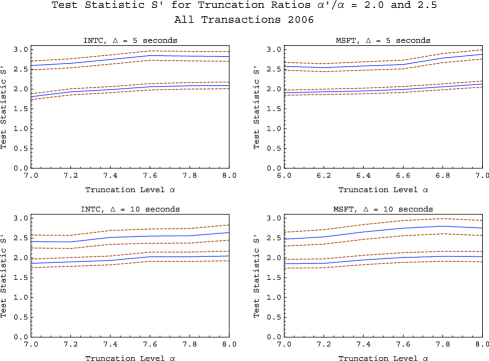
Next, we turn to the test where the null hypothesis consists of infinite jump activity. Figure 12 shows the values of the test statistic along with a confidence interval computed from the asymptotic distribution (44) under the infinite-activity null hypothesis, plotted for a range of values of the truncation index . The two curves correspond to values of equal to and respectively. The test statistic is implemented with and using seconds in the upper panels, and seconds in the lower panels. Recall from Theorem 4 that under the null of infinite activity, should go to and , respectively, for the two curves, and to under the alternative of finite activity. We find that is close to the predicted value which leads us to not reject the null hypothesis of infinite activity.
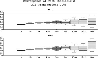
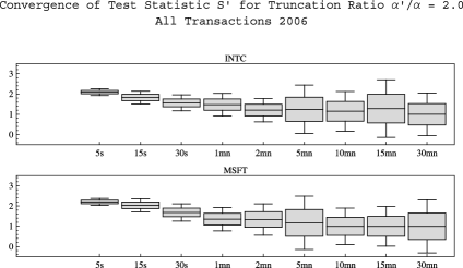
To summarize, the answer from both tests appears indicative of infinite jump activity in those data: using we reject the null of finite activity, while using we do not reject the null of infinite activity. Finally, we illustrate in Figure 13 the convergence of to as the sampling interval decreases, indicating that the null hypothesis of finite activity is rejected when high-frequency data (of the order of seconds) are used. On the other hand, we see that using longer sampling intervals (of the order of minutes) makes it impossible to reject the null hypothesis of finite activity using This is compatible with the fact that small jumps occurring over short time intervals can be aggregated or smoothed out over longer time intervals. For the second testing situation, Figure 14 shows the convergence of to as the sampling interval decreases from minutes to seconds, indicating that the null hypothesis of infinite activity is not rejected at high frequency. As in the first test, lower frequency data tend to be more compatible with finite jump activity. In both cases, longer sampling intervals over the same sampling length lead to a reduction in the sample size which generally leads to an increase in the variance of the test statistic, making it more difficult ceteris paribus to reject the null hypothesis.
Acknowledgments
We are very grateful to a referee, an Associate Editor and the Editor for many helpful comments.
Supplement to “Testing whether jumps have finite or infinite activity” \slink[doi]10.1214/11-AOS873SUPP \sdatatype.pdf \sfilenameaos873_suppl.pdf \sdescriptionThis supplementary article contains a few additional technical details about the assumptions made in this paper, and the proofs of all results.
References
- Aït-Sahalia (2002) {barticle}[auto:STB—2011-03-03—12:04:44] \bauthor\bsnmAït-Sahalia, \bfnmY.\binitsY. (\byear2002). \btitleTelling from discrete data whether the underlying continuous-time model is a diffusion. \bjournalJ. Finance \bvolume57 \bpages2075–2112. \endbibitem
- Aït-Sahalia and Jacod (2009a) {barticle}[auto:STB—2011-03-03—12:04:44] \bauthor\bsnmAït-Sahalia, \bfnmY.\binitsY. and \bauthor\bsnmJacod, \bfnmJ.\binitsJ. (\byear2009a). \btitleEstimating the degree of activity of jumps in high frequency financial data. \bjournalAnn. Statist. \bvolume37 \bpages2202–2244. \endbibitem
- Aït-Sahalia and Jacod (2009b) {barticle}[mr] \bauthor\bsnmAït-Sahalia, \bfnmYacine\binitsY. and \bauthor\bsnmJacod, \bfnmJean\binitsJ. (\byear2009b). \btitleTesting for jumps in a discretely observed process. \bjournalAnn. Statist. \bvolume37 \bpages184–222. \biddoi=10.1214/07-AOS568, issn=0090-5364, mr=2488349 \endbibitem
- Aït-Sahalia and Jacod (2011) {bmisc}[auto:STB—2011-03-03—12:04:44] \bauthor\bsnmAït-Sahalia, \bfnmY.\binitsY. and \bauthor\bsnmJacod, \bfnmJ.\binitsJ. (\byear2011). \bhowpublishedSupplement to “Testing whether jumps have finite or infinite activity.” DOI:10.1214/11-AOS873SUPP. \endbibitem
- Andersen, Bollerslev and Diebold (2007) {barticle}[auto:STB—2011-03-03—12:04:44] \bauthor\bsnmAndersen, \bfnmT. G.\binitsT. G., \bauthor\bsnmBollerslev, \bfnmT.\binitsT. and \bauthor\bsnmDiebold, \bfnmF. X.\binitsF. X. (\byear2007). \btitleRoughing it up: Including jump components in the measurement, modeling, and forecasting of return volatility. \bjournalRev. Econom. Statist. \bvolume89 \bpages701–720. \endbibitem
- Ball and Torous (1983) {barticle}[auto:STB—2011-03-03—12:04:44] \bauthor\bsnmBall, \bfnmC. A.\binitsC. A. and \bauthor\bsnmTorous, \bfnmW. N.\binitsW. N. (\byear1983). \btitleA simplified jump process for common stock returns. \bjournalJournal of Financial and Quantitative Analysis \bvolume18 \bpages53–65. \endbibitem
- Barndorff-Nielsen and Shephard (2004) {barticle}[auto:STB—2011-03-03—12:04:44] \bauthor\bsnmBarndorff-Nielsen, \bfnmO. E.\binitsO. E. and \bauthor\bsnmShephard, \bfnmN.\binitsN. (\byear2004). \btitlePower and bipower variation with stochastic volatility and jumps (with discussion). \bjournalJournal of Financial Econometrics \bvolume2 \bpages1–48. \endbibitem
- Bates (1991) {barticle}[auto:STB—2011-03-03—12:04:44] \bauthor\bsnmBates, \bfnmD. S.\binitsD. S. (\byear1991). \btitleThe crash of ’87: Was it expected? The evidence from options markets. \bjournalJ. Finance \bvolume46 \bpages1009–1044. \endbibitem
- Belomestny (2010) {barticle}[mr] \bauthor\bsnmBelomestny, \bfnmDenis\binitsD. (\byear2010). \btitleSpectral estimation of the fractional order of a Lévy process. \bjournalAnn. Statist. \bvolume38 \bpages317–351. \biddoi=10.1214/09-AOS715, issn=0090-5364, mr=2589324 \bptnotecheck year \endbibitem
- Carr and Wu (2003a) {barticle}[auto:STB—2011-03-03—12:04:44] \bauthor\bsnmCarr, \bfnmP.\binitsP. and \bauthor\bsnmWu, \bfnmL.\binitsL. (\byear2003a). \btitleThe finite moment log stable process and option pricing. \bjournalJ. Finance \bvolume58 \bpages753–777. \endbibitem
- Carr and Wu (2003b) {barticle}[auto:STB—2011-03-03—12:04:44] \bauthor\bsnmCarr, \bfnmP.\binitsP. and \bauthor\bsnmWu, \bfnmL.\binitsL. (\byear2003b). \btitleWhat type of process underlies options? A simple robust test. \bjournalJ. Finance \bvolume58 \bpages2581–2610. \endbibitem
- Carr et al. (2002) {barticle}[auto:STB—2011-03-03—12:04:44] \bauthor\bsnmCarr, \bfnmP.\binitsP., \bauthor\bsnmGeman, \bfnmH.\binitsH., \bauthor\bsnmMadan, \bfnmD. B.\binitsD. B. and \bauthor\bsnmYor, \bfnmM.\binitsM. (\byear2002). \btitleThe fine structure of asset returns: An empirical investigation. \bjournalJournal of Business \bvolume75 \bpages305–332. \endbibitem
- Cont and Mancini (2009) {bmisc}[auto:STB—2011-03-03—12:04:44] \bauthor\bsnmCont, \bfnmR.\binitsR. and \bauthor\bsnmMancini, \bfnmC.\binitsC. (\byear2009). \bhowpublishedNonparametric tests for probing the nature of asset price processes. Technical report, Univ. Firenze. \endbibitem
- Eberlein and Keller (1995) {barticle}[auto:STB—2011-03-03—12:04:44] \bauthor\bsnmEberlein, \bfnmE.\binitsE. and \bauthor\bsnmKeller, \bfnmU.\binitsU. (\byear1995). \btitleHyperbolic distributions in finance. \bjournalBernoulli \bvolume1 \bpages281–299. \endbibitem
- Huang and Tauchen (2005) {barticle}[auto:STB—2011-03-03—12:04:44] \bauthor\bsnmHuang, \bfnmX.\binitsX. and \bauthor\bsnmTauchen, \bfnmG. T.\binitsG. T. (\byear2005). \btitleThe relative contribution of jumps to total price variance. \bjournalJournal of Financial Econometrics \bvolume4 \bpages456–499. \endbibitem
- Jacod and Shiryaev (2003) {bbook}[mr] \bauthor\bsnmJacod, \bfnmJean\binitsJ. and \bauthor\bsnmShiryaev, \bfnmAlbert N.\binitsA. N. (\byear2003). \btitleLimit Theorems for Stochastic Processes, \bedition2nd ed. \bseriesGrundlehren der Mathematischen Wissenschaften [Fundamental Principles of Mathematical Sciences] \bvolume288. \bpublisherSpringer, \baddressBerlin. \bidmr=1943877 \endbibitem
- Jacod et al. (2009) {barticle}[mr] \bauthor\bsnmJacod, \bfnmJean\binitsJ., \bauthor\bsnmLi, \bfnmYingying\binitsY., \bauthor\bsnmMykland, \bfnmPer A.\binitsP. A., \bauthor\bsnmPodolskij, \bfnmMark\binitsM. and \bauthor\bsnmVetter, \bfnmMathias\binitsM. (\byear2009). \btitleMicrostructure noise in the continuous case: The pre-averaging approach. \bjournalStochastic Process. Appl. \bvolume119 \bpages2249–2276. \biddoi=10.1016/j.spa.2008.11.004, issn=0304-4149, mr=2531091 \endbibitem
- Jiang and Oomen (2008) {barticle}[mr] \bauthor\bsnmJiang, \bfnmGeorge J.\binitsG. J. and \bauthor\bsnmOomen, \bfnmRoel C. A.\binitsR. C. A. (\byear2008). \btitleTesting for jumps when asset prices are observed with noise—a “swap variance” approach. \bjournalJ. Econometrics \bvolume144 \bpages352–370. \biddoi=10.1016/j.jeconom.2008.04.009, issn=0304-4076, mr=2526151 \endbibitem
- Lee and Hannig (2010) {bmisc}[auto:STB—2011-03-03—12:04:44] \bauthor\bsnmLee, \bfnmS. S.\binitsS. S. and \bauthor\bsnmHannig, \bfnmJ.\binitsJ. (\byear2010). \bhowpublishedDetecting jumps from Lévy jump diffusion processes. Journal of Financial Economics 96 271–290. \endbibitem
- Lee and Mykland (2008) {barticle}[auto:STB—2011-03-03—12:04:44] \bauthor\bsnmLee, \bfnmS.\binitsS. and \bauthor\bsnmMykland, \bfnmP. A.\binitsP. A. (\byear2008). \btitleJumps in financial markets: A new nonparametric test and jump dynamics. \bjournalReview of Financial Studies \bvolume21 \bpages2535–2563. \endbibitem
- Madan, Carr and Chang (1998) {barticle}[auto:STB—2011-03-03—12:04:44] \bauthor\bsnmMadan, \bfnmD. B.\binitsD. B., \bauthor\bsnmCarr, \bfnmP. P.\binitsP. P. and \bauthor\bsnmChang, \bfnmE. E.\binitsE. E. (\byear1998). \btitleThe Variance Gamma process and option pricing. \bjournalEuropean Finance Review \bvolume2 \bpages79–105. \endbibitem
- Madan and Seneta (1990) {barticle}[auto:STB—2011-03-03—12:04:44] \bauthor\bsnmMadan, \bfnmD. B.\binitsD. B. and \bauthor\bsnmSeneta, \bfnmE.\binitsE. (\byear1990). \btitleThe Variance Gamma (V.G.) model for share market returns. \bjournalJournal of Business \bvolume63 \bpages511–524. \endbibitem
- Mancini (2001) {barticle}[auto:STB—2011-03-03—12:04:44] \bauthor\bsnmMancini, \bfnmC.\binitsC. (\byear2001). \btitleDisentangling the jumps of the diffusion in a geometric jumping Brownian motion. \bjournalGiornale dell’Istituto Italiano degli Attuari \bvolumeLXIV \bpages19–47. \endbibitem
- Merton (1976) {barticle}[auto:STB—2011-03-03—12:04:44] \bauthor\bsnmMerton, \bfnmR. C.\binitsR. C. (\byear1976). \btitleOption pricing when underlying stock returns are discontinuous. \bjournalJournal of Financial Economics \bvolume3 \bpages125–144. \endbibitem
- Todorov and Tauchen (2010) {barticle}[mr] \bauthor\bsnmTodorov, \bfnmViktor\binitsV. and \bauthor\bsnmTauchen, \bfnmGeorge\binitsG. (\byear2010). \btitleActivity signature functions for high-frequency data analysis. \bjournalJ. Econometrics \bvolume154 \bpages125–138. \biddoi=10.1016/j.jeconom.2009.06.009, issn=0304-4076, mr=2558956 \endbibitem