TU-926

Algorithms to Evaluate Multiple Sums
for Loop Computations

C. Anzai and Y. Sumino
Department of Physics, Tohoku University
Sendai, 980-8578 Japan

We present algorithms to evaluate two types of multiple sums, which appear in higher-order loop computations. We consider expansions of a generalized hyper-geometric-type sums, $\sum_{n_{1},\cdots,n_{N}}\frac{\Gamma(\boldsymbol{a}_{1}\cdot\boldsymbol{n}+c_{1})\Gamma(\boldsymbol{a}_{2}\cdot\boldsymbol{n}+c_{2})\cdots\Gamma(\boldsymbol{a}_{P}\cdot\boldsymbol{n}+c_{P})}{\Gamma(\boldsymbol{b}_{1}\cdot\boldsymbol{n}+d_{1})\Gamma(\boldsymbol{b}_{2}\cdot\boldsymbol{n}+d_{2})\cdots\Gamma(\boldsymbol{b}_{Q}\cdot\boldsymbol{n}+d_{Q})}~{}x_{1}^{n_{1}}\cdots x_{N}^{n_{N}}\rule[-8.53581pt]{0.0pt}{21.33955pt}~{}~{}$ with $\boldsymbol{a}_{i}\!\cdot\!\boldsymbol{n}=\sum_{j=1}^{N}a_{ij}n_{j}\rule[-8.53581pt]{0.0pt}{14.22636pt}$, etc., in a small parameter $\epsilon$ around rational values of $c_{i}$,$d_{i}$’s. Type I sum corresponds to the case where, in the limit $\epsilon\to 0$, the summand reduces to a rational function of $n_{j}$’s times $x_{1}^{n_{1}}\cdots x_{N}^{n_{N}}$; $c_{i}$,$d_{i}$’s can depend on an external integer index. Type II sum is a double sum ($N=2$), where $c_{i},d_{i}$’s are half-integers or integers as $\epsilon\to 0$ and $x_{i}=1$; we consider some specific cases where at most six $\Gamma$ functions remain in the limit $\epsilon\to 0$. The algorithms enable evaluations of arbitrary expansion coefficients in $\epsilon$ in terms of $Z$-sums and multiple polylogarithms (generalized multiple zeta values). We also present applications of these algorithms. In particular, Type I sums can be used to generate a new class of relations among generalized multiple zeta values. We provide a Mathematica package, in which these algorithms are implemented.

1 Introduction

During the last decades, there have been remarkable developments in technologies for computing higher-order radiative corrections in quantum field theories. Applications of these computational technologies extend from phenomenology of particle physics to various fields of theoretical research; see, for instance, reviews [1, 2, 3, 4, 5, 6, 7].

It has become a standard procedure to reduce numerous integrals, which appear in higher-order corrections, to a small set of integrals (master integrals) using identities derived by integration by parts [8] or other types of identities. One of the themes of today’s computational technologies for evaluating master integrals concerns how to reduce a class of transcendental functions of the form

$$F(c_{1},\dots,c_{P};d_{1},\dots,d_{Q};x_{1},\dots,x_{N})$$

$$~{}~{}~{}=\sum_{n_{1},\cdots,n_{N}}\frac{\Gamma(\boldsymbol{a}_{1}\!\cdot\!\boldsymbol{n}+c_{1})\Gamma(\boldsymbol{a}_{2}\!\cdot\!\boldsymbol{n}+c_{2})\cdots\Gamma(\boldsymbol{a}_{P}\!\cdot\!\boldsymbol{n}+c_{P})}{\Gamma(\boldsymbol{b}_{1}\!\cdot\!\boldsymbol{n}+d_{1})\Gamma(\boldsymbol{b}_{2}\!\cdot\!\boldsymbol{n}+d_{2})\cdots\Gamma(\boldsymbol{b}_{Q}\!\cdot\!\boldsymbol{n}+d_{Q})}~{}x_{1}^{n_{1}}\cdots x_{N}^{n_{N}}$$ (1)

with $\boldsymbol{a}_{i}\!\cdot\!\boldsymbol{n}=a_{i,1}n_{1}+\cdots+a_{i,N}n_{N}$, etc. Generally, $c_{i}$’s and $d_{i}$’s depend linearly on a small expansion parameter $\epsilon$, and the expansion coefficients in $\epsilon$ need to be computed. The goal of the reduction is an expression in terms of some simpler mathematical objects whose properties are well known and which are amenable to fast high-precision numerical evaluations. Mathematical functions that have been explored for this purpose are the harmonic sum, nested harmonic sum [9], polylogarithm, harmonic polylogarithms (HPLs) [10], multiple polylogarithm [11], and their generalizations [12, 13]; special values of these functions, such as multiple zeta values (MZVs) [14] and their generalizations [15, 12, 13], also take part.

The problem becomes more and more intricate as the order of loops is raised or as the number of scales involved increases. Typically in eq. (1), the summation multiplicity $N$ becomes large, more $\Gamma$ functions appear, more entangled combinations of the indices $n_{1},\dots,n_{N}$ appear in the arguments of $\Gamma$ functions, and expansions of $c_{i}$’s and $d_{i}$’s around more complicated rational numbers and to higher orders in $\epsilon$ become requisite.

There have been systematic studies on reduction of single sums ($N=1$) of the form of eq. (1) [16, 12, 17, 18, 19, 20]. By contrast, studies on reduction of multiple sums ($N\geq 2$) are still premature: The methods of recursion relations [21], of differential equations [22], and of summation [12, 23] have been examined and applied to computations of multi-loop integrals. What class of multiple sums can be reduced? And to which extent can they be reduced? Which method is more efficient or general? — Studies on these questions seem to have a long way ahead.

In this paper, we present algorithms to evaluate two types of multiple sums, each of which corresponds to an arbitrary expansion coefficient in $\epsilon$ of a sub-class of the above multiple sum. Type I sum corresponds to the case where the ratio of the $\Gamma$ functions in the summand of eq. (1) reduces to a rational function of $n_{j}$’s in the limit $\epsilon\to 0$, with integer coefficients of $n_{j}$’s in each linear polynomial factor. Furthermore, $c_{i},d_{i}$’s can depend on an external integer index $\nu$ linearly, through which the sum becomes dependent on $\nu$. The algorithm can reduce the expansion coefficients at any order in $\epsilon$ and for any summation multiplicity. The result of reduction is expressed in terms of $Z$-sums (generalized nested harmonic sums) and their values at infinity (multiple polylogarithms), which depend on $x_{1},\dots,x_{N}$.

Type II sum is a double sum with the form $\sum_{\ell,m=0}^{\infty}\prod_{p}\frac{\Gamma\left(\ell+a_{p}\right)}{\Gamma\left(\ell+b_{p}\right)}\prod_{q}\frac{\Gamma\left(m+c_{q}\right)}{\Gamma\left(m+d_{q}\right)}\prod_{r}\frac{\Gamma\left(\ell+m+e_{r}\right)}{\Gamma\left(\ell+m+f_{r}\right)}$, where $a_{p},\dots,f_{r}$ are half-integers (including integers), and for $p,q,r\geq 2$, the ratios of $\Gamma$ functions reduce to rational functions of $\ell,m$ as $\epsilon\to 0$. This means that at most six $\Gamma$ functions remain as $\epsilon\to 0$. The algorithm can reduce the expansion coefficients at any order in $\epsilon$. The result of reduction is expressed in terms of generalized MZVs. We give precise definitions for the two types of sums in the main body of the paper.

Each type of sum covers a broad class of multiple sums and has useful applications. In particular, we can use Type I sum in the following ways: (a) to convert a non-nested integral to a combination of nested integrals, and (b) to derive a new type of relations among the generalized MZVs, which can be useful in reducing expressions of final results. We also apply the algorithms to compute master integrals for a static QCD potential at three-loop order. We present two new results.

Our algorithm for evaluating Type I sum is similar to the one developed in [23] (see also [24]), which is an algorithm adapted to evaluating a wide class of multiple sums for loop computations. The algorithm of [23] uses solutions to difference equations for transforming a multiple sum to a combination of nested sums (which may later be expressed by harmonic sums, multiple polylogarithms, etc.) The method works if there are solutions to difference equations in the solution space in which they are searched for. At present, however, in many cases one has to make explicit trials to see which class of sums can eventually be transformed to nested sums. Specifically, it has been unknown whether Type I sum can be converted to nested sums in general cases. On the other hand, in our algorithm, we convert Type I sum to nested sums using the method of differences combined with the invariance of the summand under shifts of indices, in a recursive manner. This corresponds to constructing explicitly the solution to the difference equations with appropriate initial conditions, in terms of $Z$-sums and multiple polylogarithms, in the general case. Thus, our algorithm provides an existence proof of the solutions to the difference equations for Type I sums in general. Furthermore, our algorithm evaluates the sums fairly efficiently.

Type II sums can be regarded as generalizations of the sums considered in [25, 26, 17, 20], for the special values corresponding to $x_{j}=1$. These previous studies evaluate expansion coefficients of similar transcendental sums around half-integer values of their arguments (not necessarily for $x_{j}=1$), but they consider the cases where at most one pair of $\Gamma$ functions remains in the summand after expansion (binomial sums or inverse-binomial sums). In contrast, we consider the cases where at most three pairs of $\Gamma$ functions remain, whose arguments include entanglement of the indices essential to a double sum. This adds significant complexity for evaluation of the sums in comparison to the previous works.

In higher-order loop computations, more and more complicated classes of transcendental functions (and their special values) appear. In view of this general tendency, we use somewhat loose terminology in referring to generalizations of MZVs and HPLs, such as colored MZVs, cyclotomic numbers, etc. We simply refer to them as generalized MZVs or simply MZVs hereafter, and in the case that we focus particularly on their functional dependence on $\beta_{1}$ (the upper bound of the outermost integral in integral representation), we refer to them as (generalized) HPLs, although they are essentially the same quantities; they also belong to a certain class of multiple polylogarithms. See App. A for the definitions.

The paper is organized as follows. In Sec. 2, we present the algorithm for reduction of Type I sums (Algorithm I). Some applications of this algorithm are shown in Sec. 3. We present the algorithm for reduction of Type II sums (Algorithm II) in Sec. 4. Sec. 5 provides applications of Algorithm II. Summary and discussion are given in Sec. 6. We deliver definitions and conventions in App. A. Some details of Algorithm II are explained in App. B.

2 Algorithm I: Multiple Sum without $\Gamma$ Functions

In this section we present an algorithm (Algorithm I) to reduce an $N$-ple sum of the following form:

$$S(\nu)=\sum_{i_{1}=a_{1}(\nu)}^{b_{1}(\nu)}\sum_{i_{2}=a_{2}(\nu,i_{1})}^{b_{2}(\nu,i_{1})}\cdots\sum_{i_{N}=a_{N}(\nu,i_{1},\dots,i_{N-1})}^{b_{N}(\nu,i_{1},\dots,i_{N-1})}~{}\frac{\lambda_{1}^{i_{1}}\cdots\lambda_{N}^{i_{N}}}{\prod_{r}L_{r}(\nu,i_{1},\dots,i_{N})^{p_{r}}},$$ (2)

where $\nu$ is an integer. This includes, as a special case, in which $S$ does not depend on $\nu$. In eq. (2), $\lambda_{n}\in\mathbb{C}$; each factor in the denominator $L_{r}(\nu,i_{1},\dots,i_{N})$ is a linear polynomial of $\nu$ and $i_{1},\dots,i_{N}$ with integer coefficients; $p_{r}\in\mathbb{N}$; the upper or lower bound in each summation, $a_{n}$ or $b_{n}$, is either infinity or a linear polynomial of its arguments with integer coefficients. We assume that, if $\nu$ is within an appropriate range, the sum $S(\nu)$ is finite, namely, the summand is finite for any values of the indices and the sum converges if some of $a_{n},b_{n}$ are infinity. After the reduction $S(\nu)$ is expressed in terms of simple nested sums [generalized MZVs and $Z$-sums].

For clarity, we give simple examples:

$$\sum_{k=1}^{\infty}\sum_{m=1}^{\infty}\frac{1}{(k+m)^{2}(2m+4k+1)}=4-2{\cal C}\pi-\frac{\pi^{2}}{6}-4\log 2+\frac{21}{4}\zeta(3),$$ (3)

$$\sum_{k=1}^{\infty}\sum_{m=1}^{k}\frac{(-1)^{k+m}}{(k+1)^{2}(2m+1)}=-8\,{\rm Im}[Z(\infty;2,1;-i,i)]+4{\cal C}\log 2-\frac{\pi^{3}}{8}-\frac{\pi^{2}}{12},$$ (4)

$$\sum_{n=0}^{\infty}\sum_{m=0}^{\infty}\frac{1}{(1+n+\nu)^{2}(1+m+n+\nu)(m+n+1)}$$

$$~{}~{}~{}~{}~{}~{}~{}~{}~{}~{}~{}~{}~{}~{}~{}~{}~{}~{}~{}=\frac{2}{\nu}Z(\nu;3;1)+\frac{1}{\nu}Z(\nu;1,2;1,1)-\frac{\pi^{2}}{6\nu}Z(\nu;1;1),$$ (5)

where ${\cal C}=\sum_{k=0}^{\infty}\frac{(-1)^{k}}{(2k+1)^{2}}$ denotes the Catalan constant; $\zeta(z)=\sum_{n=1}^{\infty}\frac{1}{n^{z}}$ denotes the Riemann zeta function; $Z(\infty;a_{1},\cdots,a_{N};b_{1},\cdots,b_{N})$ and $Z(\nu;a_{1},\cdots,a_{N};b_{1},\cdots,b_{N})$ represent a (generalized) MZV and $Z$-sum, respectively (see App. A for definitions).

It is convenient to use the generalized sum defined by

$$\sideset{}{{}^{\prime}}{\sum}_{k=a}^{b}f\left(k\right)=\begin{cases}{\displaystyle~{}~{}~{}\sum_{k=a}^{b}f\left(k\right)}&\left(a\leq b\right)\rule[-19.91692pt]{0.0pt}{17.07164pt}\\ ~{}~{}~{}~{}~{}0&\left(a=b+1\right)\rule[-8.53581pt]{0.0pt}{17.07164pt}\\ {\displaystyle-\sum_{k=b+1}^{a-1}f\left(k\right)}&\left(a\geq b+2\right)\end{cases}$$

for integers $a$ and $b$. The relations

$$\sideset{}{{}^{\prime}}{\sum}_{k=b}^{a}f\left(k\right)=-\sideset{}{{}^{\prime}}{\sum}_{k=a+1}^{b-1}f\left(k\right),$$

$$\sideset{}{{}^{\prime}}{\sum}_{k=a+\alpha}^{k=b+\beta}f\left(k\right)=\sideset{}{{}^{\prime}}{\sum}_{k=a}^{b}f\left(k\right)+\sideset{}{{}^{\prime}}{\sum}_{k=b+1}^{b+\beta}f\left(k\right)-\sideset{}{{}^{\prime}}{\sum}_{k=a}^{a+\alpha-1}f\left(k\right)$$

hold for arbitrary integers $a,b,\alpha$ and $\beta$. Throughout this paper, it is understood that $\sum$ stands for $\sum^{\prime}$.

Let us define an integer matrix $A$ from the coefficients of $L_{r}(\nu,i_{1},\dots,i_{N})$’s by

$$A_{rn}=\frac{\partial L_{r}}{\partial i_{n}}.$$ (6)

Without loss of generality, we may assume that the rank of $A$ equals the number of the summation indices $N$. In fact, if ${\rm rank}(A)<N$, there exist redundant summation indices, namely, with an appropriate redefinition of summation indices, the summand can be rendered independent of $N\!-\!{\rm rank}(A)$ indices, and the summation over these indices can be taken trivially.

Algorithm I consists of the following steps:

1. Introduce regularization parameters if necessary and perform partial fraction decomposition of the summand.

2. Convert a multiple sum to a combination of nested sums. This is achieved by the method of differences for taking a sum of series, combined with appropriate shifts of the summation indices.

3. Remove regularization parameters and convert the nested sums to MZVs and $Z$-sums.

4. Reduce MZVs and $Z$-sums to simpler ones.

We explain each step.

Step 1

We apply partial fraction decomposition to the summand of $S(\nu)$ with respect to each summation index $i_{n}$, starting from the innermost sum, up to the outermost sum. By this procedure, $S(\nu)$ is rendered to a combination of the sums of the form eq. (2) (apart from coefficients independent of $i_{1},\dots,i_{N}$), with $N$ factors in the denominator, $L_{1},\dots,L_{N}$. Here, $L_{1}$ is independent of $i_{2},\dots,i_{N}$,  $L_{2}$ is independent of $i_{3},\dots,i_{N}$,  $\dots$,  and $L_{N-1}$ is independent of $i_{N}$. The matrix $A$ is therefore rendered to an $N\times N$ lower triangular matrix.

The partial fraction decompositions may generate divergent terms. By way of example:

$$\sum_{i_{1},i_{2},i_{3}}\frac{1}{(i_{1}+i_{2})(i_{1}+i_{3})(i_{2}+i_{3})}=\sum_{i_{1},i_{2},i_{3}}\frac{1}{2i_{1}}\left[\frac{1}{i_{1}+i_{2}}+\frac{1}{i_{1}-i_{2}}\right]\left[\frac{1}{i_{2}+i_{3}}-\frac{1}{i_{1}+i_{3}}\right].$$ (7)

The term $1/(i_{1}-i_{2})$ is divergent when $i_{1}=i_{2}$, even if we restrict $i_{1},i_{2},i_{3}$ to be positive. In general cases, if divergent terms are generated, we introduce regularization parameters $\delta_{n}$ and shift $i_{n}\to i_{n}+\delta_{n}$. At a later stage of the computation (step 3), we expand the result of the computation in $\delta_{n}$. All singular terms in $\delta_{n}$ will cancel out.

Step 2

After step 1, we obtain a combination of sums, each of which has a form

$$S_{2}(\nu;\boldsymbol{\delta})=\sum_{i_{1}=a_{1}(\nu)}^{b_{1}(\nu)}\sum_{i_{2}=a_{2}(\nu,i_{1})}^{b_{2}(\nu,i_{1})}\cdots\sum_{i_{N}=a_{N}(\nu,i_{1},\dots,i_{N-1})}^{b_{N}(\nu,i_{1},\dots,i_{N-1})}\frac{\lambda_{1}^{i_{1}}\cdots\lambda_{N}^{i_{N}}}{\prod_{r=1}^{N}L_{r}(\nu,i_{1},\dots,i_{N};\boldsymbol{\delta})^{p_{r}}},$$ (8)

up to an overall coefficient independent of $i_{1},\dots,i_{N}$. Here, $\boldsymbol{\delta}=(\delta_{1},\dots,\delta_{N})$. The goal of step 2 is to convert $S_{2}$ to a combination of nested sums; a nested sum has a general form

$$\sum_{\Lambda(\nu)\geq j_{1}>\cdots>j_{M}\geq 1}f_{1}(j_{1},\boldsymbol{\delta})f_{2}(j_{2},\boldsymbol{\delta})\cdots f_{M}(j_{M},\boldsymbol{\delta}),$$ (9)

where $\Lambda(\nu)$ is either $\infty$ or a linear polynomial of $\nu$ with integer coefficients. We construct an algorithm by induction. Suppose that for multiplicity $N\leq K-1$ we have a procedure to convert the sum given by eq. (8) to a combination of nested sums. Below we show how to convert the sum with multiplicity $N=K$.

We first find a set of integers $(\Delta_{0},\Delta_{1},\dots,\Delta_{N})$ which satisfy the following two conditions:

1. For all $L_{r}$,

   $$L_{r}(\nu+\Delta_{0},i_{1}+\Delta_{1},\dots,i_{N}+\Delta_{N};\boldsymbol{\delta})=L_{r}(\nu,i_{1},\dots,i_{N};\boldsymbol{\delta}).$$ (10)

2. $\Delta_{0}\neq 0$.

From the condition (i), it follows that $\sum_{n}A_{rn}\Delta_{n}+C_{r}\Delta_{0}=0$, where $C_{r}=\partial L_{r}/\partial\nu$. Hence,

$$\Delta_{n}=-\sum_{r}(A^{-1})_{nr}\,C_{r}\Delta_{0}.$$ (11)

Since $(A^{-1})_{nr}$ are rational numbers, with an appropriate integer $\Delta_{0}\neq 0$, all $\Delta_{n}$ can be set to integers. We denote

$$\alpha_{n}=a_{n}(\nu+\Delta_{0},i_{1}+\Delta_{1},\dots,i_{n-1}+\Delta_{n-1})-a_{n}(\nu,i_{1},\dots,i_{n-1}),$$ (12)

$$\beta_{n}=b_{n}(\nu+\Delta_{0},i_{1}+\Delta_{1},\dots,i_{n-1}+\Delta_{n-1})-b_{n}(\nu,i_{1},\dots,i_{n-1}),$$ (13)

which are also integers.

Using the property (i), one can relate $S_{2}(\nu+\Delta_{0})$ to $S_{2}(\nu)$. In fact, if we define the “difference” of the two terms as

$$\Delta S_{2}(\nu)\equiv S_{2}(\nu+\Delta_{0})-\lambda S_{2}(\nu)~{}~{}~{}~{};~{}~{}~{}~{}\lambda=\prod_{n}\lambda_{n}^{\Delta_{n}},$$ (14)

we may rewrite

$$\Delta S_{2}(\nu)=\lambda\left[\sum_{i_{1}=a_{1}+\alpha_{1}}^{b_{1}+\beta_{1}}\cdots\sum_{i_{N}=a_{N}+\alpha_{N}}^{b_{N}+\beta_{N}}-\sum_{i_{1}=a_{1}}^{b_{1}}\cdots\sum_{i_{N}=a_{N}}^{b_{N}}\right]\frac{\lambda_{1}^{i_{1}}\cdots\lambda_{N}^{i_{N}}}{\prod_{r}L_{r}(\nu,i_{1},\dots,i_{N};\boldsymbol{\delta})^{p_{r}}}~{}~{}~{}$$ (15)

by shifting the indices as $i_{n}\to i_{n}+\Delta_{n}$ in $S_{2}(\nu+\Delta_{0})$. With decomposition of the sums

$$\sum_{i_{1}=a_{1}+\alpha_{1}}^{b_{1}+\beta_{1}}\cdots\sum_{i_{N}=a_{N}+\alpha_{N}}^{b_{N}+\beta_{N}}-\sum_{i_{1}=a_{1}}^{b_{1}}\cdots\sum_{i_{N}=a_{N}}^{b_{N}}$$

$$~{}~{}=\left(\sum_{i_{1}=a_{1}}^{b_{1}}-\sum_{i_{1}=a_{1}}^{a_{1}+\alpha_{1}-1}+\sum_{i_{1}=b_{1}+1}^{b_{1}+\beta_{1}}\right)\cdots\left(\sum_{i_{N}=a_{N}}^{b_{N}}-\sum_{i_{N}=a_{N}}^{a_{N}+\alpha_{N}-1}+\sum_{i_{N}=b_{N}+1}^{b_{N}+\beta_{N}}\right)-\sum_{i_{1}=a_{1}}^{b_{1}}\cdots\sum_{i_{N}=a_{N}}^{b_{N}},$$

(16)

bulk of the difference cancels. The remaining terms include at least one “surface term,” $\sum_{i_{n}=a_{n}}^{a_{n}+\alpha_{n}-1}$ or $\sum_{i_{n}=b_{n}+1}^{b_{n}+\beta_{n}}$, whose sum can be evaluated explicitly since $\alpha_{n},\beta_{n}$ are explicit numbers. Thus, the remaining terms have summation multiplicity $K-1$ or less. According to the assumption of induction, $\Delta S_{2}(\nu)$ can be expressed by a combination of nested sums, eq. (9).

We can reconstruct $S_{2}(\nu)$ by summing up an initial term $S_{2}(\nu_{0})$ and the differences $\Delta S_{2}(\nu)$ with appropriate weights. Here, $\nu_{0}$ is the remainder in division of $\nu$ by $\Delta_{0}$, i.e., $\nu\equiv\nu_{0}~{}({\rm mod}~{}\Delta_{0})$ with $0\leq\nu_{0}<\Delta_{0}$. We have

$$S_{2}(\nu)=\lambda^{(\nu-\nu_{0})/\Delta_{0}}S_{2}(\nu_{0})+\sum_{\mu=\nu_{0}}^{\nu-\Delta_{0}}{\rm Proj}(\mu,\nu_{0},\Delta_{0})\,\Delta S_{2}(\mu)\,\lambda^{(\nu-\mu-\Delta_{0})/\Delta_{0}}.$$ (17)

The projector is defined as

$${\rm Proj}(m,n,d)=\frac{1}{d}\sum_{k=1}^{d}\exp\left(2\pi ik\frac{m-n}{d}\right)=\left\{\begin{array}[]{ll}0&\text{if $m\not\equiv n~{}({\rm mod}~{}d)$}\\ 1&\text{if $m\equiv n~{}({\rm mod}~{}d)$}\end{array}\right.,$$ (20)

such that the sum in eq. (17) is taken in steps $\Delta_{0}$. Due to the presence of the projector, the upper and lower limits of the summation in the second term of eq. (17) can be replaced by $\nu-1$ and $0$, respectively.

In the first term of eq. (17), if we assign a specific value to $\nu_{0}\in\{0,1,2,\dots,\Delta_{0}-1\}$, $S_{2}(\nu_{0})$ can be converted to a nested sum. In fact, denoting $S_{2}(\nu_{0})=\sum_{i_{1}}F(i_{1})$, we may regard $i_{1}$ as an external index of a sum $F(i_{1})$ of multiplicity $K-1$; hence, $F(i_{1})$ can be converted to a combination of nested sums.

Since $\nu_{0}$ is a function of $\nu$ in eq. (17), for our purpose, we rewrite the right-hand side in the following manner: we replace $\nu_{0}$ by $\mu_{0}$, multiply by a projector which projects out the term $\mu_{0}=\nu_{0}$, and take a sum over $\mu_{0}$. Hence,

$$S_{2}(\nu)=\lambda^{\nu/\Delta_{0}}\sum_{\mu_{0}=0}^{\Delta_{0}-1}{\rm Proj}(\nu,\mu_{0},\Delta_{0})$$

$$~{}~{}~{}~{}~{}~{}~{}~{}~{}~{}~{}~{}~{}\times\Biggl{[}\lambda^{-\mu_{0}/\Delta_{0}}S_{2}(\mu_{0})+\sum_{\mu=0}^{\nu-1}{\rm Proj}(\mu,\mu_{0},\Delta_{0})\,\Delta S_{2}(\mu)\,\lambda^{-(\mu+\Delta_{0})/\Delta_{0}}\Biggr{]}.$$ (21)

$\Delta_{0}$ being an explicit number, the sum over $\mu_{0}$ can be evaluated explicitly, and the result is $\lambda^{\nu/\Delta_{0}}$ times a combination of nested sums. Thus, apart from $\nu$ dependent coefficients which multiply individual terms, $S_{2}(\nu)$ is converted to a combination of nested sums.

Let us present a simple example:

$$f(m)=\sum_{k=1}^{\infty}\frac{(-1)^{k}}{(1+k+m)^{2}}.$$ (22)

This can be expressed as

$$f(m)=[f(m)+f(m-1)]-[f(m-1)+f(m-2)]$$

$$~{}~{}~{}~{}~{}~{}~{}~{}~{}~{}+\cdots+(-1)^{m}[f(2)+f(1)]-(-1)^{m}f(1)$$

$$~{}~{}~{}~{}~{}~{}~{}=\sum_{j=2}^{m}(-1)^{m-j}[f(j)+f(j-1)]-(-1)^{m}f(1).$$ (23)

Bulk of the sum in the “difference” of two adjacent terms gets canceled since the shifts $m\to m-1,~{}k\to k+1$ leave the denominator in eq. (22) unchanged:

$$f(j)+f(j-1)=\left(\sum_{k=1}^{\infty}-\sum_{k=2}^{\infty}\right)\frac{(-1)^{k}}{(k+j)^{2}}=\frac{-1}{(j+1)^{2}}.$$ (24)

Thus,

$$f(m)=(-1)^{m}\sum_{j=2}^{m}\frac{(-1)^{1-j}}{(j+1)^{2}}-(-1)^{m}\sum_{k=1}^{\infty}\frac{(-1)^{k}}{(k+2)^{2}}.$$ (25)

In the first term, apart from the coefficient $(-1)^{m}$, dependence on the external index $m$ enters only through the upper bound of the summation, while the second term, apart from $(-1)^{m}$, is free of $m$ and is essentially an MZV.

The above relation can be used to convert a double sum without an external index to a combination of nested sums:

$$\sum_{m=1}^{\infty}\sum_{k=1}^{\infty}\frac{(-1)^{k}\,i^{m}}{(2+m)^{2}(1+k+m)^{2}}=\sum_{m=1}^{\infty}\frac{i^{m}f(m)}{(2+m)^{2}}$$

$$~{}~{}~{}=-\sum_{m=1}^{\infty}\frac{(-i)^{m}}{(2+m)^{2}}\sum_{j=2}^{m}\frac{(-1)^{j}}{(j+1)^{2}}-\sum_{m=1}^{\infty}\frac{(-i)^{m}}{(2+m)^{2}}\sum_{k=1}^{\infty}\frac{(-1)^{k}}{(k+2)^{2}}.$$ (26)

The first term in the last line is essentially a nested sum, while the second term is a product of single sums.

Step 3

We convert the nested sums obtained in step 2 to MZVs and $Z$-sums. Up to an overall coefficient independent of the summation indices, each nested sum has a form

$$S_{3}(\nu;\boldsymbol{\delta})=\sum_{\Lambda(\nu)\geq j_{1}>\cdots>j_{M}\geq 0}\frac{\lambda_{1}^{j_{1}}}{(j_{1}+q_{1}+\boldsymbol{c}_{1}\cdot\boldsymbol{\delta})^{p_{1}}}\times\cdots\times\frac{\lambda_{M}^{j_{M}}}{(j_{M}+q_{M}+\boldsymbol{c}_{M}\cdot\boldsymbol{\delta})^{p_{M}}},$$ (27)

where $\boldsymbol{c}_{n}=(c_{n,1},\dots,c_{n,N})$ and $c_{n,r},q_{n}\in\mathbb{Q}$. We have normalized the coefficient of each summation index $j_{n}$ to unity in each factor in the denominator.

First we convert all the offsets $q_{n}$’s to integers. Let $\ell$ be the least common multiple (LCM) of the denominators of $q_{1},\dots,q_{M}$. In eq. (27), we may replace $j_{n}$ by $j_{n}/\ell$ and insert ${\rm Proj}(j_{n},0,\ell)$ for each $n$, such that each sum is taken on multiples of $\ell$:

$$S_{3}(\nu;\boldsymbol{\delta})=\sum_{\ell\Lambda(\nu)\geq j_{1}>\cdots>j_{M}\geq 0}~{}\prod_{n=1}^{M}\frac{{\rm Proj}(j_{n},0,\ell)\,\lambda_{n}^{j_{n}}\,\ell^{p_{n}}}{(j_{n}+\ell q_{n}+\ell\boldsymbol{c}_{n}\cdot\boldsymbol{\delta})^{p_{n}}}.$$ (28)

Expanding the projector eq. (20), $S_{3}$ is given by a combination of nested sums with integer offsets $\ell q_{n}$.

Next we shift each index $j_{n}\to j_{n}-\ell q_{n}$ to eliminate the offset. By this procedure, divergent terms as $\delta_{n}\to 0$ are explicitly taken outside of the summation. Then we expand in $\delta_{n}$’s [up to ${\cal O}(\delta_{n}^{0})$] the terms taken outside of the summation as well as the summands. All the divergent terms (which include negative powers of $\delta_{n}$’s) cancel out. Finally, by repeated applications of shifts of summation indices, shifts of upper and lower bounds of sums, and partial fraction decompositions, we can convert all the sums to $Z$-sums [with argument $n\nu$ ($n\in\mathbb{N}$)] and MZVs.

In the case that some of $\Lambda(\nu)$’s are $\infty$, divergent MZVs as $j_{n}\to\infty$ may appear in individual sums. By regularizing the sums carefully for large values of $j_{n}$’s, these divergences can be extracted from individual terms and they cancel out. For instance, if we adopt a cut-off regularization, $\Lambda(\nu)=\infty\to\Lambda(\nu)=\Lambda\gg 1$, at most logarithmic divergences $\sim(\log\Lambda)^{P}$ appear. A shift of index $j_{n}$ alters neither divergent part or the finite part as $\Lambda\to\infty$. A multiplication of the cut-off in eq. (28) induces a change $(\log\Lambda)^{P}\to(\log\Lambda+\log\ell)^{P}$, hence, this effect must properly be taken into account.

We give an example to illustrate the step 3:

$$\sum_{k=1}^{\nu}\frac{1}{k-1+\delta}\sum_{m=1}^{k}\frac{1}{m+1/2}=\sum_{k=1}^{2\nu}\frac{{\rm Proj}(k,0,2)}{k/2-1+\delta}\sum_{m=1}^{k}\frac{{\rm Proj}(m,0,2)}{m/2+1/2}$$

$$=\sum_{k=1}^{2\nu}\frac{1+(-1)^{k}}{k-2+2\delta}\sum_{m=1}^{k}\frac{1+(-1)^{m}}{m+1}=\frac{2}{3\delta}+\sum_{k=3}^{2\nu}\frac{1+(-1)^{k}}{k-2+2\delta}\sum_{m=1}^{k}\frac{1+(-1)^{m}}{m+1}$$

$$=\frac{2}{3\delta}+\frac{52}{9}-\frac{2}{3\nu}-\frac{4}{3(1+2\nu)}-\frac{Z(2\nu;1;1)-Z(2\nu;1;-1)}{\nu}$$

$$~{}~{}~{}~{}~{}~{}-2Z(2\nu;1;1)+\frac{10}{3}Z(2\nu;1;-1)+Z(2\nu;1,1;1,1)-Z(2\nu;1,1;1,-1)$$

$$~{}~{}~{}~{}~{}~{}+Z(2\nu;1,1;-1,1)-Z(2\nu;1,1;-1,-1)+{\cal O}(\delta).$$ (29)

In the last equality, a straightforward but somewhat cumbersome computation is needed to convert the sum to a combination of $Z$-sums.

Step 4

In many cases, host of MZVs and $Z$-sums are included in the result of the step 3. They can be expressed by small sets of basis elements for MZVs and $Z$-sums through specific reduction procedures or by utilizing known database. Reductions of MZVs and $Z$-sums using various relations among them, such as shuffle relations, have been studied extensively in the literatures, and we do not discuss them here; see [27, 13] and references therein. We apply such reduction procedures to simplify the result. (We can also derive non-trivial relations among MZVs using the algorithm given in this section. This will be discussed in Sec. 3.2.)

Comment on surface terms at infinity

In the case that some of the upper bounds of the summation in eq. (2) are infinity, the partial fraction decompositions in step 1 may generate logarithmically divergent sums as $j_{n}\to\infty$. This causes some subtleties to contributions of the “surface terms,” which appear in step 2. For convergent sums, the surface terms from $j_{n}\to\infty$ certainly vanish. It is a priori not obvious, however, whether contributions of the surface terms vanish in the case that there are individually divergent sums. By way of example, consider a convergent sum ($=1$):

$$\sum_{k=1}^{\infty}\sum_{n=1}^{\infty}\frac{1}{k(k+n)(k+n+1)}=\sum_{k=1}^{\infty}\sum_{n=1}^{\infty}\frac{1}{k}\left(\frac{1}{k+n}-\frac{1}{k+n+1}\right).$$ (30)

If we separate the sum on the right-hand side, each sum becomes logarithmically divergent. Let us replace the upper bounds by a cut-off $\Lambda\gg 1$ and convert the first sum $\sum_{k=1}^{\Lambda}\frac{f(k)}{k}$, with $f(k)=\sum_{n=1}^{\Lambda}\frac{1}{k+n}$, to a nested sum by

$$f(k)=f(1)+\sum_{j=2}^{k}[f(j)-f(j-1)]=f(1)+\sum_{j=2}^{k}\left(\frac{1}{j+\Lambda}-\frac{1}{j}\right).$$ (31)

Thus, the contribution of the surface term at $j=\Lambda$ is given by

$$\sum_{k=1}^{\Lambda}\frac{1}{k}\sum_{j=2}^{k}\frac{1}{j+\Lambda}=\frac{\pi^{2}}{12}~{}~{}~{}~{}\mbox{as $\Lambda\to\infty$, }$$ (32)

which is indeed non-vanishing. It turns out that the contribution of the surface term from the second term of eq. (30) exactly cancels eq. (32). Hence, the contributions of the surface terms vanish as a whole. This would not be surprising, since the sum eq. (30) is convergent as $k\to\infty$. Instead, if we introduce different cut-offs $\Lambda_{k}$ and $\Lambda_{n}$ for $k$ and $n$, respectively, and take the limit $\Lambda_{n}\to\infty$ first, we readily find that the individual surface terms vanish.

In general, this problem of the surface terms can be treated properly by introducing cut-off regularization as above. In a particular regularization scheme and in the case that all $|\lambda_{n}|=1$, we can argue that the surface terms from $j_{n}=\infty$ vanish (provided the computation is carried out in a specific order, see below), so that these surface terms can be ignored in the computation. This reduces the amount of computation considerably, as compared to other regularization schemes, in which one has to trace contributions of the surface terms through the computation.

The argument goes as follows. Suppose that, in the original sum $S$ [eq. (2)], the upper bounds of the summation indices $i_{n_{r}}$ for $r=1,2,\dots,N^{\prime}(\leq N)$ are infinity. We replace the upper bounds of these indices by $\Lambda_{n_{r}}$, respectively. $S$ is convergent as each $\Lambda_{n_{r}}\to\infty$. For convenience, let us denote the external index $\nu$ as $i_{0}$. The surface terms are contained in $\Delta S_{2}$, eq. (15). Since we apply the algorithm in step 2 recursively to convert sums with lower multiplicities, the argument $i_{x}$ of $S_{2}$ or $\Delta S_{2}$ is not necessarily an external index ($i_{0}$) but generally it can also be one of the summation indices $i_{n}$’s. We can always work from the outermost to innermost sum in applying the algorithm, such that any of the indices corresponding to the surface terms in $\Delta S_{2}$, $i_{n}$, is inner with respect to the argument $i_{x}$ of $\Delta S_{2}$, namely, $x<n$ for all the summation indices $i_{n}$’s contained in $S_{2}(i_{x})$. Consider the contribution of only one surface term at $i_{n_{r}}=\Lambda_{n_{r}}$ to $\Delta S_{2}$: it is suppressed by $\Lambda_{n_{r}}^{-p}$ with $p\geq 1$; contributions of sums of indices other than $i_{n_{r}}$ diverge at most logarithmically $\sim\prod_{s\neq r}(\log\Lambda_{n_{s}})^{P_{s}}$. If the index $i_{x}$ reaches up to order $\Lambda_{x}$, the sum of $\Delta S_{2}(i_{x})$ over $i_{x}$ is at most order $\Lambda_{x}/\Lambda_{n_{r}}^{p}\times\prod_{s\neq r}(\log\Lambda_{n_{s}})^{P_{s}}$. Therefore, if we parametrize all the cut-offs by a single parameter $u$ as $\Lambda_{n_{r}}=u^{n_{r}}$ and take a limit $u\to\infty$, the cut-offs corresponding to inner indices diverge faster ($\Lambda_{x}\ll\Lambda_{n_{r}}$), so that the contribution of the surface term vanishes. (The outer sums modify the dependence on $u$ at most logarithmically, which does not alter vanishing of the surface term contribution.) The contribution of more than one surface term vanishes even faster with $u$.

To summarize, in the case that all $|\lambda_{n}|=1$, if we work from the outermost sum to innermost sum in converting non-nested sums to combinations of nested sums (if we do not exchange the order of summation indices), we can neglect contributions of the surface terms at infinity.

3 Applications of Algorithm I

3.1 Conversion of Non-nested Integral to Nested Integrals

The algorithm given in the previous section (Algorithm I) converts a certain type of non-nested sums to combinations of nested sums. A straightforward application of this algorithm is to convert a certain type of non-nested integrals to a combination of nested integrals such as HPLs. In fact, in problems suited to manipulations in integral representations, it is often useful to convert a non-nested multiple integral to a combination of nested integrals.

There are multiple integrals (with one external parameter $x$) which can be converted to multiple sums of the form

$$F(x)=\sum_{\nu=1}^{\infty}\frac{x^{\nu}}{\nu^{P}}\,S(\nu)\,{\rm Proj}(\nu,0,d)~{}~{}~{}~{};~{}~{}~{}~{}P\in\mathbb{N},$$ (33)

by first expanding the integrand in Taylor series and then integrating. Here, $S(\nu)$ is given by eq. (2). This may occur in the case that the integrand is a combination of a rational function, logarithms, and HPLs of the integral variables. We can use Algorithm I to convert $S(\nu)$ to a combination of nested sums; in this form $F(x)$ is expressed as a combination of nested integrals straightforwardly. We give a simple example for illustration:

$$I(x)=\int^{x}_{0}dy\,\log(1-y/x)\,\log(1-xy)=\int^{x}_{0}dy\,\sum_{k=1}^{\infty}\frac{(y/x)^{k}}{k}\sum_{m=1}^{\infty}\frac{(xy)^{m}}{m}$$

$$~{}~{}~{}~{}~{}=\sum_{m=1}^{\infty}\frac{x^{1+2m}}{m}\sum_{k=1}^{\infty}\frac{1}{k(k+m+1)}=\sum_{m=1}^{\infty}\frac{x^{1+2m}}{m}\left[\frac{1}{(m+1)^{2}}+\frac{Z(m;1;1)}{m+1}\right].$$ (34)

In the last step we applied Algorithm I. Using standard relations among MZVs and HPLs, we may express the above result in terms of HPLs:

$$I(x)=2x-\frac{1-x^{2}}{x}\Bigl{[}Z(\infty;1;x^{2})+Z(\infty;2;x^{2})+Z(\infty;1,1;x^{2},1)\Bigr{]}$$

$$~{}~{}~{}=2x+\frac{1-x^{2}}{x}\Bigl{[}H_{-1}(x)+H_{1}(x)-H_{-1,-1}(x)-H_{-1,1}(x)$$

$$~{}~{}~{}~{}~{}~{}~{}~{}~{}~{}~{}~{}~{}~{}~{}~{}~{}~{}~{}~{}~{}~{}~{}~{}~{}+2H_{0,-1}(x)+2H_{0,1}(x)-H_{1,-1}(x)-H_{1,1}(x)\Bigr{]}.$$ (35)

This is a combination of nested integrals; see eqs. (69)–(71) for the definition of HPL.

In more general cases, one may need to redefine the summation indices appropriately, so that the exponent of $x$ is expressed in terms of a single index. For instance, we redefine $k+n=l$ in

$$\sum_{k=1}^{\infty}\sum_{n=1}^{\infty}x^{k+n}F\left(k,n\right)=\sum_{l=2}^{\infty}x^{l}\,\sum_{n=1}^{l-1}F\left(l-n,n\right),$$ (36)

and convert the inner sum to a combination of $Z$-sums with arguments $ml$ $(m\in\mathbb{N})$.

Examples of integrals, which can be converted to combinations of nested integrals in a similar manner, and which may be useful, are given by

$$I_{1}(x)=\int^{x}_{0}dy\,y^{p(1)}\,(\log y)^{p(2)}\,[\log(1-y)]^{p(3)}\,[\log(1+y)]^{p(4)}$$

$$~{}~{}~{}~{}~{}~{}~{}~{}~{}~{}~{}~{}~{}~{}~{}~{}~{}\times[\log(1-y/x)]^{p(5)}\,[\log(1-xy)]^{p(6)}\,H(y),$$ (37)

$$I_{2}(w)=\int_{0}^{w}dx\int_{0}^{x}dy\int_{0}^{y}dz\,x^{p(1)}y^{p(2)}z^{p(3)}\left[\log\left(1-{xy}/{w}\right)\right]^{p(4)}$$

$$~{}~{}~{}~{}~{}~{}~{}~{}~{}~{}~{}~{}~{}~{}~{}~{}~{}~{}~{}~{}~{}~{}~{}~{}~{}~{}~{}\times\left[\log\left(1-{yz}/{w}\right)\right]^{p(5)}\left[\log\left(1-{zx}/{w}\right)\right]^{p(6)},$$ (38)

where $p(n)\in\mathbb{N}$, and $H(y)$ is an HPL. The resulting expressions, however, may be quite lengthy.

3.2 Relations among MZVs

As already stated, a number of relations among MZVs have been derived and used for expressing MZVs by a set of basis elements. We show that Algorithm I can be used to derive yet another type of relations among (generalized) MZVs.

We demonstrate it using an example. Suppose that $\lambda\in\mathbb{C}$ satisfies

$$|\lambda|\leq 1~{}~{}~{}\mbox{and}~{}~{}~{}\lambda\neq 1.$$ (39)

We rearrange the order of the summation of a weight-two MZV:

$$Z(\infty;1,1;\lambda,-\lambda)=\sum_{n>m>0}\frac{\lambda^{n}(-\lambda)^{m}}{nm}=\sum_{s=3}^{\infty}\sum_{m=1}^{\left\lfloor\frac{s-1}{2}\right\rfloor}\lambda^{s}\,\frac{(-1)^{m}}{m(s-m)}$$

$$~{}~{}~{}~{}~{}~{}=\sum_{r=1}^{\infty}\lambda^{2r+1}\sum_{m=1}^{r}\frac{(-1)^{m}}{m(2r+1-m)}+\sum_{r=1}^{\infty}\lambda^{2r+2}\sum_{m=1}^{r}\frac{(-1)^{m}}{m(2r+2-m)}.$$ (40)

We set $s=n+m$. The upper bound of $m$ follows from the condition $m\leq n-1=s-m-1$, where $\lfloor x\rfloor$ denotes the greatest integer less than or equal to $x$. In the last line we separate $s$ to odd and even numbers and set $s=2r+1$ and $s=2r+2$, respectively. The sums over $m$ can be converted to combinations of $Z$-sums by Algorithm I. It can be shown that the above rearrangement of summation is justified under the condition eq. (39). Thus, we find a relation among MZVs:

$$z(\lambda,-\lambda)=-\frac{1}{2}z(-2\lambda^{2})+\frac{3}{4}z(-\lambda,-1)-z(-\lambda,-i)-z(-\lambda,i)-\frac{1}{4}z(-\lambda,1)$$

$$~{}~{}~{}~{}~{}~{}~{}~{}~{}~{}~{}~{}~{}~{}-\frac{1}{4}z(\lambda,-1)+z(\lambda,-i)+z(\lambda,i)-\frac{1}{4}z(\lambda,1)+\frac{1}{4}z(\lambda^{2},1).$$ (41)

We use a short-hand notation for MZV, eq. (68), where the original forms can be reproduced via $z(x_{1},\dots,x_{n})\to Z(\infty;\alpha_{1},\dots,\alpha_{n};\beta_{1},\dots,\beta_{n})$ with $\alpha_{i}=|x_{i}(\lambda=1)|$ and $\beta_{i}=x_{i}/\alpha_{i}$. The relation eq. (41) may be regarded as a special case of the conversion relation described in Sec. 3.1.

In particular, in the case that $\lambda^{n}\!=\!\pm i$ for some $n\in\mathbb{N}$, eq. (41) may lead to an interesting relation. We have examined independence of the above relation from other relations, such as shuffle relations and those which can be derived by variable transformations in integral representations of MZVs (e.g. $x\to x^{-1}$, $x\to x^{2}$, $x\to\frac{1+ix^{2}}{1-ix^{2}}$). In the case that $\lambda=\pm i$, eq. (41) does not give a new relation. On the other hand, in the case $\lambda=e^{i\pi/4}$ (a primitive 8th root of unity), it gives a new relation, which can be used for reduction of MZVs. In fact, this gives a relation between the three basis elements at $w=2$, $l=8$ proposed in [13]:

$$-3i\,{{\rm Im}[{\rm Li}_{2}(e_{8})]}+3{\sigma_{1,1}(e_{8},e_{4})}+{\sigma_{1,1}(e_{8},e_{8}^{3})}+2i{\cal C}+\frac{53\pi^{2}}{192}$$

$$~{}~{}+\frac{1}{2}\log^{2}\Bigl{(}\sqrt{2}\!-\!1\Bigr{)}-\frac{\log^{2}2}{8}-\frac{5}{4}\log 2\,\log\Bigl{(}\sqrt{2}\!-\!1\Bigr{)}+\frac{9}{16}i\pi\log 2=0.$$ (42)

Therefore, the number of the (new) basis elements reduces to two.

It is easy to obtain relations among MZVs in more complicated cases, by rearranging summation orders using this method. The strategy is to rewrite an MZV $Z(\infty;\alpha_{1},\dots,\alpha_{n};\beta_{1},\dots,\beta_{n})$, for which some of $|\beta_{i}|$’s are the same (equal to $|\lambda|$), in a combination of HPLs of the type $H_{a_{1},\dots,a_{n}}(\omega\lambda^{m})$ (MZVs with $\beta_{1}=\omega\lambda^{m}$). Here, $\omega$ denotes a root of unity.

Up to now, we do not know whether these relations can be derived from other known methods. Extensive exploration of the relations among MZVs for the case beyond $\beta_{i}=\pm 1$ (e.g. $n$-th root of unity for $n>2$) is still underway [15, 28, 13]. We expect that the above method would be a useful tool for analyses in this direction. We have checked in specific examples that they lead to relations independent of shuffle relations and are powerful in reducing MZVs to a small set of elements. Generally, a huge set of relations need to be generated, which requires an efficient algorithm for generation of the relations, and Algorithm I is useful in this respect.

3.3 Evaluation of a 3-Loop Master Integral

We apply Algorithm I for evaluating a 3-loop integral

$${\cal M}_{1}=\int\frac{d^{D}p}{(2\pi)^{D}}\frac{d^{D}k}{(2\pi)^{D}}\frac{d^{D}\kappa}{(2\pi)^{D}}\,\frac{1}{(k\cdot v)(p\cdot v)k^{2}p^{2}(k+q)^{2}(p+q)^{2}(k+\kappa)^{2}(p+\kappa)^{2}}.$$ (43)

This is one of the 40 master integrals, which appear in a computation of the 3-loop correction to the static QCD potential ($\bar{a}_{3}$) [29, 30]; the diagram is shown in Fig. 1. In dimensional regularization ($D=4-2\epsilon$), expansion coefficients of ${\cal M}_{1}$ in $\epsilon$ up to (and including) order $\epsilon$ is necessary. In eq. (43), we omit $+i0$ in the propagator denominators, hence, {$k\cdot v$, $k^{2}$, $(k+q)^{2}$, $\dots$} stand for {$k\cdot v+i0$, $k^{2}+i0$, $(k+q)^{2}+i0$, $\dots$}; $q=(0,\vec{q})$ is a spacelike external momentum, whereas $v=(1,\vec{0})$ is a temporal unit vector; $(k\cdot v+i0)^{-1}$ represents a heavy-quark propagator.

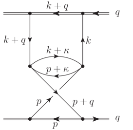
Figure 1: Diagram for the master integral ${\cal M}_{1}$. Double lines represent heavy-quark propagators, while single lines represent massless propagators.

Using a standard technology [2], such as the one described in [31], one can convert the above integral to a three-fold Mellin-Barnes integral. Closing the contour in the complex plane for each Mellin-Barnes integral variable, one may further convert the integral to a combination of three-fold sums with $\Gamma$ functions. By expanding in $\epsilon$, at every order of $\epsilon$ all the $\Gamma$ functions cancel, and we are left with sums of the form eq. (2). We evaluate the expansion coefficients up to ${\cal O}(\epsilon)$ using Algorithm I, where sums with multiplicity up to six need to be evaluated. The result is given by

$${\cal M}_{1}=A(\epsilon)(-q^{2})^{-1-3\epsilon}\times\left[\frac{\pi^{4}}{\epsilon}+\biggl{\{}-93\zeta(5)-14\pi^{2}\zeta(3)+\pi^{4}\Bigl{(}2+6\log 2\Bigr{)}\biggr{\}}\right.$$

$$~{}~{}~{}~{}~{}~{}~{}~{}~{}~{}~{}~{}+\epsilon\,\biggl{\{}-288s_{6}-186\zeta(5)+234\zeta(3)^{2}+\pi^{2}\Bigl{(}96\text{Li}_{4}\bigl{(}{\textstyle\frac{1}{2}}\bigr{)}-28\zeta(3)+4\log^{4}2\Bigr{)}$$

$$~{}~{}~{}~{}~{}~{}~{}~{}~{}~{}~{}~{}~{}~{}~{}~{}~{}~{}~{}+\pi^{4}\Bigl{(}4+12\log 2+14\log^{2}2\Bigr{)}+\frac{293\pi^{6}}{420}\biggr{\}}\Biggr{]},$$ (44)

$$A(\epsilon)=-i\,(4\pi)^{3\epsilon-6}\exp(-3\gamma_{E}\epsilon),$$ (45)

where $\gamma_{E}=0.5772...$ denotes the Euler constant; $s_{6}=z(-5,-1)+\zeta(6)=\sum_{m\geq n\geq 1}\frac{(-1)^{m+n}}{m^{5}n}=0.9874414264...$; ${\rm Li}_{n}(x)=\sum_{k=1}^{\infty}\frac{x^{k}}{k^{n}}$ denotes polylogarithm. We have checked the above result numerically by evaluating Feynman parameter integral representation using sector decomposition. This result has not been published elsewhere.

4 Algorithm II: Expansion Coefficients of Double Sum with $\Gamma$ Functions

We consider a double sum

$$K(\boldsymbol{a},\boldsymbol{b};\boldsymbol{c},\boldsymbol{d};\boldsymbol{e},\boldsymbol{f})=\sum_{\ell=0}^{\infty}\sum_{m=0}^{\infty}\Biggl{[}\prod_{p=1}^{L}\frac{\Gamma\left(\ell+a_{p}\right)}{\Gamma\left(\ell+b_{p}\right)}\Biggr{]}\Biggl{[}\prod_{q=1}^{M}\frac{\Gamma\left(m+c_{q}\right)}{\Gamma\left(m+d_{q}\right)}\Biggr{]}\Biggl{[}\prod_{r=1}^{N}\frac{\Gamma\left(\ell+m+e_{r}\right)}{\Gamma\left(\ell+m+f_{r}\right)}\Biggr{]},$$

(46)

where $\boldsymbol{a}=(a_{1},\dots,a_{L})$, etc. In this section we present an algorithm (Algorithm II) for computing expansion coefficients of $K$ in a small parameter around integer or half-integer arguments. We assume the following conditions for the arguments of $K$:

1. $\boldsymbol{a}=\boldsymbol{a}_{0}+\epsilon\boldsymbol{a}_{1}$, $\dots$, $\boldsymbol{f}=\boldsymbol{f}_{0}+\epsilon\boldsymbol{f}_{1}$, where $a_{0,p},b_{0,p},c_{0,q},d_{0,q},e_{0,r},f_{0,r}$ are half-integers (including integers) and $\epsilon$ is a small expansion parameter. $a_{1,p},b_{1,p},c_{1,q},d_{1,q},e_{1,r},f_{1,r}$ are complex variables used to parametrize the expansion coefficients.

2. For $p,q,r\geq 2$, $a_{0,p}-b_{0,p}$, $c_{0,q}-d_{0,q}$, $e_{0,r}-f_{0,r}$ are integers.

3. The sum in eq. (46) is convergent at $(\boldsymbol{a}_{0},\boldsymbol{b}_{0};\boldsymbol{c}_{0},\boldsymbol{d}_{0};\boldsymbol{e}_{0},\boldsymbol{f}_{0})$, hence $K$ is regular with respect to $\boldsymbol{a}_{1},\dots,\boldsymbol{f}_{1}$ as $\epsilon\to 0$.

The algorithm reduces an arbitrary expansion coefficient of $K$ in $\epsilon$, up to any order, to a combination of MZVs. Due to the above conditions, there remain at most six uncanceled $\Gamma$ functions in the summand in each expansion coefficient, before reduction.

We give an example:

$$\frac{\partial}{\partial\epsilon}\frac{\partial}{\partial\delta}\frac{\partial^{2}}{\partial\alpha^{2}}\,C(\epsilon,\delta,\alpha)\!\sum_{k,m=0}^{\infty}\frac{\Gamma(k\!+\!1)\Gamma(m\!+\!1)\Gamma(k\!+\!m\!+\!\frac{3}{2})\Gamma(k\!+\!m\!+\!\epsilon\!+\!2)}{\Gamma(k\!+\!\alpha\!+\!\frac{5}{2})\Gamma(m\!+\!\frac{5}{2})\Gamma(k\!+\!m\!+\!2)\Gamma(k\!+\!m\!+\!\delta\!+\!3)}\Biggr{|}_{\epsilon,\delta,\alpha\to 0}$$

$$=-7296s_{6}-\frac{508\pi^{6}}{63}+\pi^{4}\left(-8\log^{2}2+\frac{32\log 2}{45}+\frac{292}{15}\right)+\pi^{2}\Biggl{\{}\zeta({3})\left(56\log 2+\frac{656}{3}\right)$$

$$~{}~{}~{}+\frac{152\log^{4}2}{3}+192\log^{3}2+\frac{416\log^{2}2}{3}+\frac{32\log 2}{3}+192\text{Li}_{4}\bigl{(}{\textstyle\frac{1}{2}}\bigr{)}-\frac{80}{3}\Biggr{\}}+972\zeta({3})^{2}$$

$$~{}~{}~{}+\zeta({5})(6882\log 2+22318)+\zeta({3})(-448\log^{3}2-2024\log^{2}2-752\log 2-248)$$

$$~{}~{}~{}-\frac{1024\log^{6}2}{15}-\frac{3808\log^{5}2}{15}-\frac{32\log^{4}2}{3}+\frac{1024\log^{3}2}{3}+\log^{2}2\Bigl{(}-3072\text{Li}_{4}\bigl{(}{\textstyle\frac{1}{2}}\bigr{)}+192\Bigr{)}$$

$$~{}~{}~{}+\log 2\Bigl{(}-9216\text{Li}_{5}\bigl{(}{\textstyle\frac{1}{2}}\bigr{)}-8320\text{Li}_{4}\bigl{(}{\textstyle\frac{1}{2}}\bigr{)}-160\Bigr{)}$$

$$~{}~{}~{}-12288\text{Li}_{6}\bigl{(}{\textstyle\frac{1}{2}}\bigr{)}-11136\text{Li}_{5}\bigl{(}{\textstyle\frac{1}{2}}\bigr{)}-256\text{Li}_{4}\bigl{(}{\textstyle\frac{1}{2}}\bigr{)}-144,$$ (47)

where we have included a prefactor $C(\epsilon,\delta,\alpha)={\Gamma(\delta\!+\!3)\Gamma(\alpha\!+\!\frac{5}{2})}/{\Gamma(\epsilon\!+\!2)}$ in order to eliminate trivial $\gamma_{E}$ and $\sqrt{\pi}$.

The algorithm consists of the following steps:

1. Convert $K$ to an integral representation.

2. Apply Kummer’s formula and other variable transformations to simplify the integral and to eliminate half-integer powers in the integrand.

3. Expand in $\epsilon$. If necessary, regularize appropriately before the expansion.

4. Convert multiple integrals to combinations of nested integrals. Integrals with respect to individual integral variables are converted recursively. In each conversion process, we extract singularities using integration by parts, remove regularization parameters, and apply Algorithm I. In the end the result is expressed by MZVs.

5. Reduce MZVs to simpler ones.

We explain each step below.

Step 1

For later convenience, we denote

$$e_{r}=e^{\prime}_{N+1-r},~{}~{}~{}f_{r}=f^{\prime}_{N+1-r}~{}~{}~{}~{}(1\leq r\leq N).$$ (48)

We express each pair of $\Gamma$ functions using the integral representation of the beta function as

$$\frac{\Gamma\left(\ell+a_{p}\right)}{\Gamma\left(\ell+b_{p}\right)}=\frac{1}{\Gamma(b_{p}-a_{p})}\int_{0}^{1}dx_{p}\,x_{p}^{\ell+a_{p}-1}(1-x_{p})^{b_{p}-a_{p}-1},$$ (49)

$$\frac{\Gamma\left(m+c_{q}\right)}{\Gamma\left(m+d_{q}\right)}=\frac{1}{\Gamma(d_{q}-c_{q})}\int_{0}^{1}dy_{q}\,y_{q}^{m+c_{q}-1}(1-y_{q})^{d_{q}-c_{q}-1},$$ (50)

$$\frac{\Gamma\left(\ell+m+e^{\prime}_{r}\right)}{\Gamma\left(\ell+m+f^{\prime}_{r}\right)}=\frac{1}{\Gamma(f^{\prime}_{r}-e^{\prime}_{r})}\int_{0}^{1}dz_{r}\,z_{r}^{\ell+m+e^{\prime}_{r}-1}(1-z_{r})^{f^{\prime}_{r}-e^{\prime}_{r}-1}.$$ (51)

Hence, we obtain an integral representation

$$K\propto\int_{0}^{1}\!\!dx_{1}\cdots\int_{0}^{1}\!\!dx_{L}~{}\int_{0}^{1}\!\!dy_{1}\cdots\int_{0}^{1}\!\!dy_{M}~{}\int_{0}^{1}\!\!dz_{1}\cdots\int_{0}^{1}\!\!dz_{N}~{}$$

$$~{}~{}~{}~{}~{}~{}~{}\times\frac{\prod_{p}x_{p}^{a_{p}-1}(1-x_{p})^{b_{p}-a_{p}-1}\prod_{q}y_{q}^{c_{q}-1}(1-y_{q})^{d_{q}-c_{q}-1}\prod_{r}z_{r}^{e^{\prime}_{r}-1}(1-z_{r})^{f^{\prime}_{r}-e^{\prime}_{r}-1}}{(1-x_{1}\cdots x_{L}z_{1}\cdots z_{N})(1-y_{1}\cdots y_{M}z_{1}\cdots z_{N})}.$$

(52)

Step 2

We apply Kummer’s formula

$$\int_{0}^{1}\!dt\,\frac{t^{\alpha}(1-t)^{\beta}}{(1-tT)^{\gamma}}=\frac{\Gamma(\alpha+1)\Gamma(\beta+1)}{\Gamma(\gamma)\Gamma(\alpha\!+\!\beta\!-\!\gamma\!+\!2)}\frac{(1-T)^{\beta-\gamma+1}}{T^{\alpha+\beta-\gamma+2}}\int_{0}^{T}\!\!dt\,\frac{t^{\alpha+\beta-\gamma+1}}{(1-t)^{\beta+1}}\biggl{(}1\!-\!\frac{t}{T}\biggr{)}^{\!\gamma-1}$$

(53)

for $\gamma=1$ to the variables $t=x_{1}$ and $y_{1}$ of eq. (52). Next we apply the following variable transformations successively (here, $\zeta_{i}$’s denote the new variables and not zeta values):

• $z_{N}=\zeta_{N}$, and $z_{i}=\zeta_{i}/\zeta_{i+1}$ starting from $i=N-1$ to $i=1$.

• $x_{1}=\xi_{1}$, $x_{L}=\xi_{L}/\zeta_{1}$, and $x_{i}=\xi_{i}/\xi_{i+1}$ starting from $i=L-1$ to $i=2$.

• $y_{1}=\eta_{1}$, $y_{M}=\eta_{M}/\zeta_{1}$, and $y_{i}=\eta_{i}/\eta_{i+1}$ starting from $i=M-1$ to $i=2$.

This leads to an integral representation of $K$, where the integral variables are ordered as depicted in Fig. 2, and where

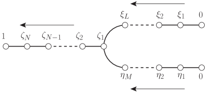
Figure 2: Diagram showing the order of the integral variables. Along the same line, the variables to the left are larger. The order of $\xi_{p}$ and $\eta_{q}$ is not fixed.

each factor of the integrand contains at most two (adjacent) integral variables:

$$K\propto{\hbox to18.0pt{ \hbox to-3.0pt{$\displaystyle\int$} \raise-18.0pt\hbox{$\scriptstyle 1\geq\zeta_{N}\geq\cdots\geq\zeta_{1}\geq 0$} }}\!d\zeta_{N}\cdots d\zeta_{1}~{}{\hbox to18.0pt{ \hbox to-3.0pt{$\displaystyle\int$} \raise-18.0pt\hbox{$\scriptstyle\zeta_{1}\geq\xi_{L}\geq\cdots\geq\xi_{1}\geq 0$} }}\!d\xi_{L}\cdots d\xi_{1}~{}{\hbox to18.0pt{ \hbox to-3.0pt{$\displaystyle\int$} \raise-18.0pt\hbox{$\scriptstyle\zeta_{1}\geq\eta_{M}\geq\cdots\geq\eta_{1}\geq 0$} }}\!d\eta_{M}\cdots d\eta_{1}~{}~{}\zeta_{1}^{e^{\prime}_{1}-a_{L}-c_{M}-1}\left(1-\zeta_{N}\right)^{f^{\prime}_{N}-e^{\prime}_{N}-1}$$

$$\qquad\times\left(1\!-\!\xi_{1}\right)^{a_{1}-b_{1}}\xi_{1}^{b_{1}-2}\left(1\!-\!\xi_{2}\right)^{b_{1}-a_{1}-1}\xi_{2}^{a_{2}-b_{1}}\left(1\!-\!\eta_{1}\right)^{c_{1}-d_{1}}\eta_{1}^{d_{1}-2}\left(1\!-\!\eta_{2}\right)^{d_{1}-c_{1}-1}\eta_{2}^{c_{2}-d_{1}}\rule[0.0pt]{0.0pt}{17.07164pt}$$

$$\qquad\times\left(1-\frac{\xi_{L}}{\zeta_{1}}\right)^{b_{L}-a_{L}-1}\left(1-\frac{\eta_{M}}{\zeta_{1}}\right)^{d_{M}-c_{M}-1}\rule[0.0pt]{0.0pt}{22.76219pt}$$

$$\qquad\times\left(1-\frac{\xi_{2}}{\xi_{3}}\right)^{b_{2}-a_{2}-1}\xi_{3}^{a_{3}-a_{2}-1}\cdots\left(1-\frac{\xi_{L-1}}{\xi_{L}}\right)^{b_{L-1}-a_{L-1}-1}\xi_{L}^{a_{L}-a_{L-1}-1}$$

$$\qquad\times\left(1-\frac{\eta_{2}}{\eta_{3}}\right)^{d_{2}-c_{2}-1}\eta_{3}^{c_{3}-c_{2}-1}\cdots\left(1-\frac{\eta_{M-1}}{\eta_{M}}\right)^{d_{M-1}-c_{M-1}-1}\eta_{M}^{c_{M}-c_{M-1}-1}$$

$$\qquad\times\left(1-\frac{\zeta_{1}}{\zeta_{2}}\right)^{f^{\prime}_{1}-e^{\prime}_{1}-1}\zeta_{2}^{e^{\prime}_{2}-e^{\prime}_{1}-1}\cdots\left(1-\frac{\zeta_{N-1}}{\zeta_{N}}\right)^{f^{\prime}_{N-1}-e^{\prime}_{N-1}-1}\zeta_{N}^{e^{\prime}_{N}-e^{\prime}_{N-1}-1}.$$ (54)

We note that all the factors containing two variables have integer powers at $\epsilon=0$, according to the condition (ii) and eq. (48). On the other hand, the factors $t$ and $1-t$ for $t=\xi_{p},\eta_{q},\zeta_{r}$ have half-integer (including integer) powers at $\epsilon=0$.

We may render the exponents of all the factors of the integrand to integers (at $\epsilon=0$) using the following variable transformations. We first apply the transformation

$$t\rightarrow\frac{4t}{\left(1+t\right)^{2}}.$$ (55)

to all the variables $t=\xi_{p},\eta_{q},\zeta_{r}$ simultaneously. The integral region is unchanged, and the factors in the integrand transform as

$$1-t\rightarrow\left(\frac{1-t}{1+t}\right)^{2},\qquad 1-\frac{t}{t^{\prime}}\rightarrow\frac{\left(1-{t}/{t^{\prime}}\right)\left(1-t\,t^{\prime}\right)}{t^{\prime}\left(1+t\right)^{2}}.$$ (56)

If half-integer powers still remain, we further transform $t\to t^{2}$. This eliminates half-integer powers in the general case.

Step 3

Although $K$ is finite at $\epsilon=0$, setting $\epsilon=0$ in the integrand before integration may lead to divergences. These superficial divergences originate from the integral representations eqs. (49)–(51) and (53), in the case that some of these integrals are not well-defined around $\epsilon=0$. If there are (superficial) divergences, we introduce regularization parameters in the following manner, before expanding in $\epsilon$:

$$a_{i}\rightarrow a_{i}+\delta_{a_{1}}+\cdots+\delta_{a_{i}},~{}~{}\qquad b_{i}\rightarrow b_{i}+\delta_{a_{1}}+\cdots+\delta_{a_{i}}+\delta_{b_{i}},$$

$$c_{i}\rightarrow c_{i}+\delta_{c_{1}}+\cdots+\delta_{c_{i}},~{}~{}~{}\qquad d_{i}\rightarrow d_{i}+\delta_{c_{1}}+\cdots+\delta_{c_{i}}+\delta_{d_{i}},$$

$$e^{\prime}_{i}\rightarrow e^{\prime}_{i}+\delta_{a_{1}}+\cdots+\delta_{a_{L}}+\delta_{c_{1}}+\cdots+\delta_{c_{M}}+\delta_{e^{\prime}_{1}}+\cdots+\delta_{e^{\prime}_{i}},$$

$$f^{\prime}_{i}\rightarrow f^{\prime}_{i}+\delta_{a_{1}}+\cdots+\delta_{a_{L}}+\delta_{c_{1}}+\cdots+\delta_{c_{M}}+\delta_{e^{\prime}_{1}}+\cdots+\delta_{e^{\prime}_{i}}+\delta_{f^{\prime}_{i}}.$$ (57)

This parametrization is specially tailored for the use in step 4. As we will see, it is important that we can take the limit $\delta_{i}\to 0$ corresponding to each integral variable (each set of integral variables), without affecting outer integrals. In fact, after applying the above regularization, most exponents of the factors of the integrand depend on only one regularization parameter, respectively. For reference, in Table 1 we list the exponents in eq. (54) after applying the regularization, from which one may easily deduce the integral form after the variable transformation eq. (55) (and $t\to t^{2}$).

${e^{\prime}_{1}-a_{L}-c_{M}-1+\delta_{e^{\prime}_{1}}},$	${f^{\prime}_{N}-e^{\prime}_{N}-1+\delta_{f_{N}}},~{}~{}~{}~{}~{}~{}$	${a_{1}-b_{1}-\delta_{b_{1}}},$	${b_{1}-2+\delta_{a_{1}}+\delta_{b_{1}}},$
${b_{1}-a_{1}-1+\delta_{b_{1}}},$	${a_{2}-b_{1}+\delta_{a_{2}}-\delta_{b_{1}}},$	${c_{1}-d_{1}-\delta_{d_{1}}},$	${d_{1}-2+\delta_{c_{1}}+\delta_{d_{1}}},$
${d_{1}-c_{1}-1+\delta_{d_{1}}},$	${c_{2}-d_{1}+\delta_{c_{2}}-\delta_{d_{1}}},$	${b_{L}-a_{L}-1+\delta_{b_{L}}},$	${d_{M}-c_{M}-1+\delta_{d_{M}}},$
${b_{2}-a_{2}-1+\delta_{b_{2}}},$	${a_{3}-a_{2}-1+\delta_{a_{3}}},~{}\cdots,~{}{b_{L-1}-a_{L-1}-1+\delta_{b_{L-1}}},$		${a_{L}-a_{L-1}-1+\delta_{a_{L}}},$
${d_{2}-c_{2}-1+\delta_{d_{2}}},$	${c_{3}-c_{2}-1+\delta_{c_{3}}},~{}\cdots,~{}{d_{M-1}-c_{M-1}-1+\delta_{d_{M-1}}},$		${c_{M}-c_{M-1}-1+\delta_{c_{M}}},$
${f^{\prime}_{1}-e^{\prime}_{1}-1+\delta_{f^{\prime}_{1}}},$	${e^{\prime}_{2}-e^{\prime}_{1}-1+\delta_{e^{\prime}_{2}}},~{}\cdots,~{}{f^{\prime}_{N-1}-e^{\prime}_{N-1}-1+\delta_{f^{\prime}_{N-1}}},$		${e^{\prime}_{N}-e^{\prime}_{N-1}-1+\delta_{e^{\prime}_{N}}}.$

Table 1: Exponents of the factors of the integrand in eq. (54) after introducing regularization parameters eq. (57). The exponents of $\xi_{1},\xi_{2},\eta_{1},\eta_{2}$, respectively, depend on two regularization parameters. All other exponents, respectively, depend on a single regularization parameter.

We expand $K$ in $\epsilon$ (if necessary, after applying the above regularization). The expansion generates powers of logarithms [$\log t$, $\log(1\pm t)$, $\log(1\pm it)$, $\log(1\pm t/t^{\prime})$, $\log(1\pm t\,t^{\prime})$] in the integrand.

Step 4

We convert the integral to a sum of nested integrals using a recursive algorithm. The order of conversion is indicated by the arrows in Fig. 2: we work from the innermost integral up to the outermost integral. First we convert the double integrals with respect to the innermost variables $\xi_{1}$,$\xi_{2}$ and $\eta_{1}$,$\eta_{2}$, respectively. For the other variables, we convert the integral with respect to each variable recursively.

Let us explain how to convert the double integral with respect to $\xi_{1}$ and $\xi_{2}$. The integrand depends on the four regularization parameters $\delta_{a_{1}}$,$\delta_{a_{2}}$,$\delta_{b_{1}}$,$\delta_{b_{2}}$ (denoted by $\delta_{\xi 12}$). We note that these parameters are not included in the outer integrals. Using identities and integration by parts, we raise or decrease the exponents of the factors, $\xi_{i},1\!\pm\!\xi_{i},1\!\pm\!i\xi_{i}$ ($i=1,2$), $1\!\pm\!\xi_{2}/\xi_{3},1\!\pm\!\xi_{2}\xi_{3}$, until all of them become non-negative when $\delta_{\xi 12}$’s are set to zero. This procedure is explained in App. B. By this procedure, the double integral is converted to a sum of double integrals, where singularities in $\delta_{\xi 12}$’s are taken outside of each double integral as poles and each double integral is finite as all $\delta_{\xi 12}\to 0$. We expand $K$ in $\delta_{\xi 12}$’s up to (and including) finite terms. The poles in $\delta_{\xi 12}$’s cancel, and each double integral with respect to $\xi_{1}$ and $\xi_{2}$ is reduced to the form

$$\int_{0}^{\xi_{3}}\!\!d\xi_{2}\int_{0}^{\xi_{2}}\!\!d\xi_{1}~{}P_{\xi 12}\Bigl{(}\xi_{i},\log\xi_{i},\log(1\!\pm\!\xi_{i}),\log(1\!\pm\!i\xi_{i}),\log(1\!\pm\!\xi_{2}/\xi_{3}),\log(1\!\pm\!\xi_{2}\xi_{3})\Bigr{)}$$

where $P_{\xi 12}$ is a polynomial of its arguments. Prefactors dependent on $\xi_{3}$ may be generated, which are absorbed into the outer integral $\int d\xi_{3}$. The above integral can be converted to a combination of HPLs using Algorithm I, as described in Sec. 3.1. In fact, it is a generalized version of eq. (37).

In the same way, we convert the double integral with respect to $\eta_{1}$ and $\eta_{2}$ to a sum of HPLs.

Next we apply the following algorithm recursively from inner to outer integrals. Suppose we convert the integral with respect to $t(=\xi_{p(\geq 3)},\eta_{q(\geq 3)},\zeta_{r}$). As a result of the previous conversion, each integral has the following form:

$$\int_{0}^{t^{\prime}}\!dt~{}\left[\prod_{s=1}^{9}\phi_{s}(t,t^{\prime})^{\alpha_{s}(\delta_{1},\delta_{2})}\right]~{}{P}\Bigl{(}\log\phi_{1}(t,t^{\prime}),\dots,\log\phi_{9}(t,t^{\prime})\Bigr{)}\,H(t).$$ (59)

Here, $\phi_{s}(t,t^{\prime})$ denotes one of the nine factors $t$, $(1\pm t)$, $(1\pm it)$, $(1\pm t/t^{\prime})$, $(1\pm t\,t^{\prime})$. $P(x_{1},\dots,x_{9})$ represents a polynomial of $x_{1},\dots,x_{9}$. $H(t)$ is a nested integral which resulted from processing the inner integrals. In fact, $H(t)$ is a generalized HPL of eqs. (69)–(72). There are only two regularization parameters associated with the variable $t$, and we denote them by $\delta_{1},\delta_{2}$. In particular, $\delta_{1},\delta_{2}$ are not included in the outer integrals. The exponent $\alpha_{s}(\delta_{1},\delta_{2})$ is a linear function of $\delta_{1},\delta_{2}$, where $\alpha_{s}(0,0)$ is an integer.

We raise or decrease the exponents $\alpha_{s}(\delta_{1},\delta_{2})$’s using identities and integration by parts (see App. B). By this procedure, the original integral is converted to a combination of integrals, where singularities in $\delta_{1},\delta_{2}$ are taken outside of each integral as poles and each integral is finite as $\delta_{1},\delta_{2}\to 0$. We expand $K$ in $\delta_{1},\delta_{2}$ up to (and including) finite terms. The poles in $\delta_{1},\delta_{2}$ cancel, and each integral with respect to $t$ is reduced to the form

$$\int_{0}^{t^{\prime}}\!dt~{}\tilde{P}\Bigl{(}t,\,\log\phi_{1}(t,t^{\prime}),\,\dots,\,\log\phi_{9}(t,t^{\prime})\Bigr{)}\,H(t),$$ (60)

where $\tilde{P}$ is a polynomial of its arguments. Prefactors dependent on $t^{\prime}$ may be generated, which should be absorbed into the outer integral. The above integral can be converted to a combination of nested integrals using Algorithm I, as described in Sec. 3.1.

Finally, since the upper bound of the outermost integral is one, the result can be expressed by MZVs with roots of unity ($\beta_{i}^{P_{i}}=1$ with $P_{i}\in\mathbb{N}$).

Step 5

The same as step 4 of Algorithm I (Sec. 2).

5 Applications of Algorithm II

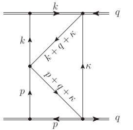
Figure 3: Diagram for the master integral ${\cal M}_{2}$. Notations are the same as in Fig. 1.

We apply Algorithm II for evaluating a 3-loop integral

$${\cal M}_{2}=\int\frac{d^{D}p}{(2\pi)^{D}}\frac{d^{D}k}{(2\pi)^{D}}\frac{d^{D}\kappa}{(2\pi)^{D}}\,\frac{1}{(k\cdot v)(p\cdot v)k^{2}p^{2}\kappa^{2}(k+q+\kappa)^{2}(p+q+\kappa)^{2}}.$$ (61)

This is another master integral necessary for a computation of $\bar{a}_{3}$; the diagram is shown in Fig. 3. The notations are the same as in Sec. 3.3.

Using Mellin-Barnes integral representation, one can express ${\cal M}_{2}$ by $K$ with five different arguments with $(L,M,N)=(1,1,2)$. After expanding in $\epsilon$, six $\Gamma$ functions remain uncanceled in the summand, for each $K$. We need to compute the expansion coefficients of $K$ around three different arguments $(a_{0,1},b_{0,1};c_{0,1},d_{0,1};e_{0,1},e_{0,2},f_{0,1},f_{0,2})=(\frac{1}{2},1;\frac{1}{2},1;\frac{1}{2},1,1,2)$, $(\frac{1}{2},1;1,\frac{3}{2};1,\frac{3}{2},\frac{3}{2},\frac{5}{2})$, $(1,\frac{3}{2};1,\frac{3}{2};\frac{3}{2},2,2,3)$ up to order $\epsilon^{5}$, $\epsilon^{3}$, $\epsilon^{3}$, respectively. We can use Algorithm II to evaluate these coefficients and obtain

$${\cal M}_{2}=A(\epsilon)(-q^{2})^{-3\epsilon}\times\Biggl{[}-\frac{28\pi^{4}}{135\epsilon}+\left\{-\frac{226\zeta(5)}{3}-\frac{116\pi^{2}\zeta(3)}{9}+\pi^{4}\left(4\log 2-\frac{224}{135}\right)\right\}$$

$$~{}~{}~{}~{}~{}+\epsilon~{}\biggl{\{}192{s_{6}}-\frac{1808\zeta(5)}{3}+\frac{8\zeta(3)^{2}}{3}+\pi^{2}\left(-64\text{Li}_{4}\bigl{(}{\textstyle\frac{1}{2}}\bigr{)}-\frac{928\zeta(3)}{9}-\frac{8}{3}\log^{4}2\right)$$

$$~{}~{}~{}~{}~{}~{}~{}~{}~{}~{}~{}~{}~{}+\pi^{4}\left(-\frac{1792}{135}+\frac{20\log^{2}2}{3}+32\log 2\right)+\frac{428\pi^{6}}{2835}\biggr{\}}$$

$$~{}~{}~{}~{}~{}+\epsilon^{2}\biggl{\{}768\text{Li}_{4}\bigl{(}{\textstyle\frac{1}{2}}\bigr{)}\zeta(3)+\frac{480}{7}\zeta(3)^{2}\log 2+1536{s_{6}}-\frac{384}{7}{s_{6}}\log 2+\frac{384}{7}s_{7a}+\frac{3072}{7}s_{7b}$$

$$~{}~{}~{}~{}~{}~{}~{}~{}~{}~{}~{}~{}~{}-\frac{4960\zeta(7)}{21}-\frac{14464\zeta(5)}{3}+\frac{64\zeta(3)^{2}}{3}+32\zeta(3)\log^{4}2-372\zeta(5)\log^{2}2$$

$$~{}~{}~{}~{}~{}~{}~{}~{}~{}~{}~{}~{}~{}+\pi^{2}\biggl{(}-512\text{Li}_{4}\bigl{(}{\textstyle\frac{1}{2}}\bigr{)}+128\text{Li}_{5}\bigl{(}{\textstyle\frac{1}{2}}\bigr{)}-\frac{7424\zeta(3)}{9}-\frac{35519\zeta(5)}{42}-32\zeta(3)\log^{2}2$$

$$~{}~{}~{}~{}~{}~{}~{}~{}~{}~{}~{}~{}~{}-\frac{16\log^{5}2}{15}-\frac{64}{3}\log^{4}2\biggr{)}+\pi^{4}\biggl{(}\frac{31457\zeta(3)}{945}-\frac{14336}{135}+\frac{40\log^{3}2}{9}$$

$$~{}~{}~{}~{}~{}~{}~{}~{}~{}~{}~{}~{}~{}+\frac{160\log^{2}2}{3}+256\log 2\biggr{)}+\pi^{6}\left(\frac{3424}{2835}+\frac{3079\log 2}{315}\right)\biggr{\}}\Biggr{]},$$ (62)

where $s_{7a}=z(-5,1,1)+z(-6,1)+z(-5,2)+z(-7)=\sum_{m\geq n\geq k\geq 1}\frac{(-1)^{m}}{m^{5}nk}=-0.9529600757562\dots$ and $s_{7b}=z(5,-1,-1)+z(7)+z(5,2)+z(-6,-1)=\sum_{m\geq n\geq k\geq 1}\frac{(-1)^{n+k}}{m^{5}nk}=1.029121262964324\dots$. We have checked the above result numerically by evaluating Feynman parameter integral representation using sector decomposition. This integral corresponds to $I_{14}$ given in [32], where ${\cal O}(\epsilon^{2})$ term is missing.

We have computed yet another master integral for $\bar{a}_{3}$ using Algorithm II. This is $I_{16}$ given in [32], where the analytical expressions for the coefficients of the $\epsilon^{-1}$ and $\epsilon^{0}$ terms are presented. Ref. [32] uses the Mellin-Barnes method in combination with PSLQ algorithm for the computation. We have reproduced their result, thus providing a cross check in a fully analytical way.

6 Summary and Discussion

We have constructed algorithms for computing two types of multiple sums (Algorithms I and II) which appear in higher-order loop computations. For instance, these types of sums appear in analytic evaluations of Mellin-Barnes integral representations by closing contours and expanding in $\epsilon$.

Algorithm I applies to a multiple sum without $\Gamma$ functions [eq. (2)]:

$$S(\nu)=\sum_{i_{1}=a_{1}(\nu)}^{b_{1}(\nu)}\sum_{i_{2}=a_{2}(\nu,i_{1})}^{b_{2}(\nu,i_{1})}\cdots\sum_{i_{N}=a_{N}(\nu,i_{1},\dots,i_{N-1})}^{b_{N}(\nu,i_{1},\dots,i_{N-1})}~{}\frac{\lambda_{1}^{i_{1}}\cdots\lambda_{N}^{i_{N}}}{\prod_{r}L_{r}(\nu,i_{1},\dots,i_{N})^{p_{r}}}.$$ (63)

The algorithm is valid for arbitrary multiplicity $N$ and works efficiently. (This is partly due to our specific regularization scheme for treating surface terms at infinity; see discussion at the end of Sec. 2.) The results are expressed by $Z$-sums [with argument $n\nu$ ($n\in\mathbb{N}$)] and generalized MZVs.

There are benefits for constructing an efficient algorithm specifically for this type of sums. First, this type of sums appear frequently in computation of expansion coefficients of loop integrals in $\epsilon$. Secondly, it has other useful applications as shown in Sec. 3: (i) Conversion of non-nested integrals to nested integrals (used in Algorithm II), (ii) Deriving non-trivial relations among MZVs; for example, we find a further reduction of the proposed basis elements at $(w,l)=(2,8)$ in [13].

Algorithm II is used to evaluate the expansion coefficients of a double sum with $\Gamma$ functions [eq. (46)],

$$K(\boldsymbol{a},\!\boldsymbol{b};\boldsymbol{c},\!\boldsymbol{d};\boldsymbol{e},\!\boldsymbol{f})=\sum_{\ell,m=0}^{\infty}\Biggl{[}\prod_{p=1}^{L}\frac{\Gamma\left(\ell\!+\!a_{p}\right)}{\Gamma\left(\ell\!+\!b_{p}\right)}\Biggr{]}\Biggl{[}\prod_{q=1}^{M}\frac{\Gamma\left(m\!+\!c_{q}\right)}{\Gamma\left(m\!+\!d_{q}\right)}\Biggr{]}\Biggl{[}\prod_{r=1}^{N}\frac{\Gamma\left(\ell\!+\!m\!+\!e_{r}\right)}{\Gamma\left(\ell\!+\!m\!+\!f_{r}\right)}\Biggr{]},$$ (64)

around half-integer values (including integer values) of its arguments $(\boldsymbol{a}_{0},\!\boldsymbol{b}_{0};\boldsymbol{c}_{0},\!\boldsymbol{d}_{0};\boldsymbol{e}_{0},\!\boldsymbol{f}_{0})$. For $p,q,r\geq 2$, $a_{0,p}-b_{0,p}$, $c_{0,q}-d_{0,q}$, $e_{0,r}-f_{0,r}$ are assumed to be integers. Hence, there remain at most six uncanceled $\Gamma$ functions in the summand in each expansion coefficient. The algorithm applies to arbitrary expansion coefficients. The results are expressed by generalized MZVs with roots of unity.

These algorithms are useful in evaluating some complicated master integrals which appear in computation of the 3-loop correction to the static QCD potential ($\bar{a}_{3}$). We have presented new results for two master integrals (Secs. 3.3 and 5).

In practical implementation of the algorithms, one can make various improvements to compute efficiently. For Algorithm I, however, at the moment we do not have ideas for essential modifications of the algorithm, apart from technical refinements. On the other hand, for Algorithm II, we may improve efficiencies non-trivially by categorizing the arguments of $K$ and changing algorithms according to the categories. Although in most difficult cases $K$ can be evaluated only by the algorithm described in Sec. 4, in simpler cases, it is possible to construct algorithms which work substantially faster: for instance, we may express $K$ in an integral representation involving hypergeometric functions ${}_{2}F_{1}$ and utilize various identities of ${}_{2}F_{1}$. We explain details of our practical implementation elsewhere.

In computation of $\bar{a}_{3}$ we encounter multiple sums which cannot be evaluated with Algorithms I and II. An example is a sum, where the arguments of $\Gamma$ functions in the numerator and denominator include the summation indices in different combinations, such as:

$$\sum_{k,m,n,\cdots}\frac{\Gamma(m+a)\Gamma(n+b)\Gamma(k+m+c)\Gamma(k+m+n+d)\cdots}{\Gamma(k+a^{\prime})\Gamma(m+n+b^{\prime})\Gamma(k+2m+n+c^{\prime})\cdots}.$$ (65)

To our knowledge, there are no known technologies which can be used to evaluate these sums in general cases. We are currently studying how to generalize the algorithms in order to evaluate these different types of sums. It may be useful to combine the present algorithms with other methods for analytical evaluation of loop integrals, such as the method of differential equation, glue-and-cut method, etc.

Appendices

Appendix A Definitions and Conventions

$Z$-sums are defined by

$$Z\left(w;\alpha_{1},\alpha_{2},\ldots,\alpha_{n};\beta_{1},\beta_{2},\ldots,\beta_{n}\right)=\sum_{w\geq k_{1}>k_{2}>\cdots>k_{n}\geq 1}\frac{\beta_{1}^{k_{1}}\beta_{2}^{k_{2}}\cdots\beta_{n}^{k_{n}}}{k_{1}^{\alpha_{1}}k_{2}^{\alpha_{2}}\cdots k_{n}^{\alpha_{n}}}$$

$$~{}~{}~{}~{}~{}~{}~{}~{}~{}~{}~{}~{}~{}~{}~{}~{}~{}~{}~{}~{}~{}~{}~{}~{}~{}~{}~{}~{}~{}~{}~{}~{}~{}~{}~{}~{}~{}~{}~{}~{}~{}~{}~{}~{}=\sum_{k_{1}=1}^{w}\frac{\beta_{1}^{k_{1}}}{k_{1}^{\alpha_{1}}}\sum_{k_{2}=1}^{k_{1}-1}\frac{\beta_{2}^{k_{2}}}{k_{2}^{\alpha_{2}}}\cdots\sum_{k_{n}=1}^{k_{n-1}-1}\frac{\beta_{n}^{k_{n}}}{k_{n}^{\alpha_{n}}},$$ (66)

where $\alpha_{i},w\in\mathbb{N}$ and $\beta_{i}\in\mathbb{C}$. For $w=\infty$, the sums are (generalized) multiple zeta values (MZVs) or multiple polylogarithms of Goncharov:

$$Z\left(\infty;\alpha_{1},\alpha_{2},\ldots,\alpha_{n};\beta_{1},\beta_{2},\ldots,\beta_{n}\right)=\mathrm{Li}_{\alpha_{n},\ldots,\alpha_{1}}\left(\beta_{n},\ldots,\beta_{1}\right).$$ (67)

We also use a short-hand notation for MZVs, in contexts where it is possible to restore the original forms:

$$Z(\infty;\alpha_{1},\dots,\alpha_{n};\beta_{1},\dots,\beta_{n})=z(\alpha_{1}\beta_{1},\dots,\alpha_{n}\beta_{n}).$$ (68)

Harmonic polylogarithms (HPLs) are defined recursively: For weight one, they are defined by

$$f_{0}\left(x\right)=\frac{1}{x},\qquad f_{\pm 1}\left(x\right)=\frac{1}{x\mp 1},$$ (69)

$$H_{0}\left(x\right)=\log\left(x\right),\qquad H_{\pm 1}\left(x\right)=\int_{0}^{x}\!dt\,\,f_{\pm 1}\left(t\right)=\log\left(1\mp x\right),$$ (70)

and for higher weights,

$$H_{\underbrace{\scriptstyle 0,\cdots,0}_{n}}(x)=\frac{1}{n!}\left[\log\left(x\right)\right]^{n},~{}~{}~{}~{}H_{a_{1},a_{2},\ldots,a_{n}}(x)=\int_{0}^{x}\!dt\,\,f_{a_{1}}(t)H(t;a_{2},\ldots,a_{n}),$$ (71)

where at least one of $a_{1},a_{2},\ldots,a_{n}$ is non-zero. The above definition can be generalized to the case

$$f_{p}(x)=\frac{1}{x-p}~{}~{}~{};~{}~{}~{}p\in\mathbb{C}$$ (72)

where $a_{i}$ of $H_{a_{1},a_{2},\ldots,a_{n}}(x)$ becomes a general complex number. We refer to it as a generalized HPL. $H_{a_{1},a_{2},\ldots,a_{n}}(x)$ is another representation of an MZV or multiple polylogarithm [eq. (67)].

Appendix B Procedure for Raising or Decreasing Exponents

In this appendix we explain the procedure used in step 4 of Algorithm II (see Sec. 4). It is used to raise or decrease the exponents of the factors in the integrand, until all of them become non-negative when the regularization parameters are set to zero.

We consider an integral of the form

$$\int_{0}^{t^{\prime}}\!dt~{}\left[\prod_{s=1}^{9}\phi_{s}(t,t^{\prime})^{\alpha_{s}(\boldsymbol{\delta})}\right]~{}{P}\Bigl{(}\log\phi_{1}(t,t^{\prime}),\dots,\log\phi_{9}(t,t^{\prime})\Bigr{)}\,H(t).$$ (73)

Here, $\phi_{s}(t,t^{\prime})$ denotes one of the nine factors $t$, $(1\pm t)$, $(1\pm it)$, $(1\pm t/t^{\prime})$, $(1\pm t\,t^{\prime})$; $P(x_{1},\dots,x_{9})$ represents a polynomial of $x_{1},\dots,x_{9}$; $H(t)$ is a generalized HPL of eqs. (69)–(72); $\boldsymbol{\delta}=(\delta_{1},\dots,\delta_{n})$ denote the regularization parameters; the exponent $\alpha_{s}(\boldsymbol{\delta})$ is a linear function of $\boldsymbol{\delta}$, where $\alpha_{s}(\boldsymbol{0})$ is an integer.

A rough sketch of the procedure is as follows. We first multiply the integrand by one, which can be decomposed as

$$1=t+(1-t)=\frac{t}{t^{\prime}}+\left(1-\frac{t}{t^{\prime}}\right)=\frac{1}{1+t^{\prime}}\,(1-t)+\frac{t^{\prime}}{1+t^{\prime}}\left(1+\frac{t}{t^{\prime}}\right),$$ (74)

etc. This is repeated until the exponents are raised sufficiently. Then we integrate by parts to trade between different exponents.

Let us explain in detail. First we select a pair of the factors $\phi_{s}$ and $\phi_{\sigma}$, for which $\alpha_{s}(\boldsymbol{0})$ and $\alpha_{\sigma}(\boldsymbol{0})$ are both negative. We multiply the integrand of eq. (73) by

$$1=c_{s}(t^{\prime})\phi_{s}(t,t^{\prime})+c_{\sigma}(t^{\prime})\phi_{\sigma}(t,t^{\prime}).$$ (75)

This is repeated $|\alpha_{s}(\boldsymbol{0})+\alpha_{\sigma}(\boldsymbol{0})|$ times. After expanding the integrand, in each term, the exponents of $\phi_{s}$ and $\phi_{\sigma}$ are both non-negative or at least one of them is non-negative. We repeat this process successively for pairs of negative exponents in each term. In the end, in each term, at most one negative exponent remains. At the same time, the sum of all the exponents are non-negative for each term. Next we perform integration by parts in every term which has $\phi_{s}^{\nu}$ with $\nu<0$, in such a way to integrate $\phi_{s}^{\nu}$. This is repeated until the exponent of $\phi_{s}$ becomes non-negative. In the end, all the exponents can be made non-negative.

In the case of a double integral with respect to $\xi_{1},\xi_{2}$, we iterate the above procedure twice, first with respect to the inner integral and then the outer integral. Due to the absence of the factors $(1\pm\xi_{1}/\xi_{2})$, $(1\pm\xi_{1}\xi_{2})$, iteration of integration by parts with respect to $\xi_{2}$ can render all the exponents non-negative. (The same is true for $\eta_{1}$,$\eta_{2}$.)

References

• [1] D. Kreimer, Phys. Rept.  363, 387 (2002) [hep-th/0010059].
• [2] V.A. Smirnov, Evaluating Feynman integrals, (STMP 211; Springer, Berlin, Heidelberg, 2004).
• [3] C. Bogner and S. Weinzierl, arXiv:0912.4364 [math-ph].
• [4] Z. Bern, J. J. M. Carrasco and H. Johansson, arXiv:0902.3765 [hep-th].
• [5] R. K. Ellis, Z. Kunszt, K. Melnikov and G. Zanderighi, Phys. Rept.  518, 141 (2012) [arXiv:1105.4319 [hep-ph]].
• [6] J. Blümlein, arXiv:1205.4991 [hep-ph].
• [7] Z. Bern, L. J. Dixon and D. A. Kosower, Sci. Am.  306N5, 20 (2012).
• [8] K. G. Chetyrkin and F. V. Tkachov, Nucl. Phys. B 192, 159 (1981).
• [9] J. Vermaseren, Int. J. Mod. Phys. A14, 2037 (1999); J. Blümlein and S. Kurth, Phys. Rev. D 60, 014018 (1999).
• [10] E. Remiddi and J. Vermaseren, Int.J.Mod.Phys. A15, 725 (2000), arXiv:hep-ph/9905237 [hep-ph].
• [11] A. B. Goncharov, Math. Res. Lett. 5, 497 (1998), http://www.math.uiuc.edu/K-theory/0297.
• [12] S. Moch, P. Uwer, and S. Weinzierl, J.Math.Phys. 43, 3363 (2002), arXiv:hep-ph/0110083 [hep-ph].
• [13] J. Ablinger, J. Blümlein, and C. Schneider, J.Math.Phys. 52, 102301 (2011), arXiv:1105.6063 [math-ph].
• [14] D. J. Broadhurst, arXiv:hep-th/9604128 [hep-th]; D. J. Broadhurst and D. Kreimer, Phys. Lett. B 393, 403 (1997) [hep-th/9609128].
• [15] D. J. Broadhurst, Eur. Phys. J. C 8, 311 (1999) [hep-th/9803091].
• [16] A. I. Davydychev, Phys. Rev. D 61, 087701 (2000) [hep-ph/9910224]; A. I. Davydychev and M. Y. Kalmykov, Nucl. Phys. B 605, 266 (2001) [hep-th/0012189].
• [17] S. Weinzierl, J.Math.Phys. 45, 2656 (2004), arXiv:hep-ph/0402131 [hep-ph].
• [18] M. Y. Kalmykov, Nucl.Phys.Proc.Suppl. 135, 280 (2004), arXiv:hep-th/0406269 [hep-th].
• [19] T. Huber and D. Maître, Comput.Phys.Commun. 175, 122 (2006), arXiv:hep-ph/0507094 [hep-ph].
• [20] M. Y. Kalmykov, B. Ward, and S. Yost, JHEP 0702, 040 (2007), arXiv:hep-th/0612240 [hep-th]; M. Y. Kalmykov and B. A. Kniehl, Nucl. Phys. B 809, 365 (2009) [arXiv:0807.0567 [hep-th]].
• [21] V. V. Bytev, M. Y. Kalmykov, and B. A. Kniehl, arXiv:1105.3565 [math-ph].
• [22] M. Y. Kalmykov and B. A. Kniehl, Phys. Lett. B 714, 103 (2012) [arXiv:1205.1697 [hep-th]].
• [23] J. Blümlein, S. Klein, C. Schneider and F. Stan, J. Symbolic Comput. 47 (2012) 1267-1289 [arXiv:1011.2656 [cs.SC]].
• [24] C. Schneider, J. Differ. Equations Appl., 11, 2005 (2002); Sem. Lothar. Combin., 56, B56b (2007); J. Symbolic Comput., 43, 611 (2008).
• [25] M. Y. Kalmykov and O. Veretin, Phys.Lett. B483, 315 (2000), arXiv:hep-th/0004010 [hep-th]; F. Jegerlehner, M. Y. Kalmykov and O. Veretin, Nucl. Phys. B 658, 49 (2003) [hep-ph/0212319].
• [26] A. I. Davydychev and M. Y. Kalmykov, Nucl. Phys. B 699, 3 (2004) [hep-th/0303162].
• [27] J. Blümlein, D. J. Broadhurst and J. A. M. Vermaseren, Comput. Phys. Commun.  181, 582 (2010) [arXiv:0907.2557 [math-ph]].
• [28] J. M. Borwein, D. J. Broadhurst, and J. Kamnitzer, Exper.Math. 10, 25 (2001), arXiv:hep-th/0004153 [hep-th].
• [29] C. Anzai, Y. Kiyo and Y. Sumino, Phys. Rev. Lett.  104, 112003 (2010) [arXiv:0911.4335 [hep-ph]]; A. V. Smirnov, V. A. Smirnov and M. Steinhauser, Phys. Rev. Lett.  104, 112002 (2010) [arXiv:0911.4742 [hep-ph]].
• [30] C. Anzai, Y. Kiyo and Y. Sumino, Nucl. Phys. B 838, 28 (2010) [arXiv:1004.1562 [hep-ph]].
• [31] V. A. Smirnov, Nucl. Phys. Proc. Suppl.  135, 252 (2004) [hep-ph/0406052]; A. V. Smirnov and V. A. Smirnov, Eur. Phys. J. C 62, 445 (2009) [arXiv:0901.0386 [hep-ph]].
• [32] A. V. Smirnov, V. A. Smirnov and M. Steinhauser, PoS RADCOR 2009, 075 (2010) [arXiv:1001.2668 [hep-ph]].
• [33] R. N. Lee and V. A. Smirnov, arXiv:1209.0339 [hep-ph].
• [34] H. Ferguson, D. Bailey, Technical Report RNR-91-032, NASA Ames (1991).