also at] Jawaharlal Nehru Centre for Advanced Scientific Research, Jakkur, Bangalore 560 064, India

Phases, transitions, and boundary conditions in a model of interacting bosons

Abstract

We carry out an extensive study of the phase diagrams of the extended Bose Hubbard model, with a mean filling of one boson per site, in one dimension by using the density matrix renormalization group and show that it contains Superfluid (SF), Mott-insulator (MI), density-wave (DW) and Haldane-insulator (HI) phases. We show that the critical exponents and central charges for the HI-DW, MI-HI and SF-MI transitions are consistent with those for models in the two-dimensional Ising, Gaussian, and Berezinskii-Kosterlitz-Thouless (BKT) universality classes, respectively; and we suggest that the SF-HI transition may be more exotic than a simple BKT transition. We show explicitly that different boundary conditions lead to different phase diagrams.

Over the last two decades, experiments on cold alkali atoms in traps have obtained various phases of correlated bosons and fermions reviews . Microscopic interaction parameters can be tuned in such experiments, which provide, therefore, excellent laboratories for studies of quantum phase transitions, such as those between superfluid (SF) and Mott-insulator (MI) phases in a system of interacting bosons in an optical lattice fisher89 ; sheshadri ; jaksch . The SF and MI phases are, respectively, the protypical examples of gapless and gapped phases in such systems; in addition, it may be possible to obtain exotic phases, e.g., density-wave (DW) kuhner98 ; rvpai05 ; entspect ; kurdestany12 , Haldane-insulator (HI) torre06 ; berg08 , and supersolid (SS) kovrizhin05 phases, in systems with a dipolar condensate of ${}^{52}{\rm Cr}$ atoms werner05 . The first step in developing an understanding of such experiments is to study lattice models of bosons with long-range interactions goral02 ; the simplest model that goes beyond the Bose-Hubbard model with onsite, repulsive interactions fisher89 ; sheshadri is the extended Bose-Hubbard model (EBHM), which allows for repulsive interactions between bosons on a site and also on nearest-neighbor sites rvpai05 ; kurdestany12 . The one-dimensional (1D) EBHM is particularly interesting because (a) quantum fluctuations are strong enough to replace long-range SF order by a quasi-long-range SF, with a power-law decay of order-parameter correlationsrvpai05 , and (b) boundary conditions play a remarkable role here, in so far as they can modify the bulk phase diagram torre06 ; berg08 ; deng12 ; rossini12 , in a way that is not normally possible in the thermodynamic limit thermodynamiclimit .

We present extensive density-matrix-renormalization-group (DMRG) rvpai05 studies of the phases, transitions, and the role of boundary conditions in the 1D EBHM with a mean filling of one boson per site. Although a few DMRG studies rvpai05 ; torre06 ; berg08 ; deng12 ; rossini12 have been carried out earlier, none of them has elucidated completely clearly the universality classes of the continuous transitions in the 1D EBHM; nor have they compared in detail, the phase diagrams of this model with different boundary conditions. Our study, which has been designed to obtain the universality classes of these transitions and to examine the role of boundary conditions in stabilizing different phases, yields a variety of interesting results that we summarize qualitatively below: If the filling $\rho=1$, in the thermodynamic limit, we obtain three types of phase diagrams, P1 (Fig. 1(a)), P2 (Fig. 1(b)), and P3 (Fig. 1(c)), for boundary conditions BC1 (number of bosons $N=L$, where $L$ is the number of sites), BC2 ($N=L+1$), and BC3 ($N=L$ and additional chemical potentials at the boundary sites, as we describe below), respectively. For P1 we obtain SF, MI, and DW phases and we confirm, as noted earlier rvpai05 , that the SF-MI transition is in the Berezinskii-Kosterlitz-Thouless (BKT) kogutreview universality class and the SF-DW has both BKT and two-dimensional (2D) Ising characteristics; at sufficiently large values of the repulsive parameters, the MI-DW transition is of first order rvpai05 . The phase diagram P2 displays SF, HI, and DW phases, with continuous SF-HI and HI-DW transitions in BKT and 2D Ising universality classes, respectively. The phase diagram P3 has SF, MI, HI, and DW phases, with SF-MI, MI-HI, HI-DW in BKT, 2D Gaussian gaussian1 , and 2D Ising universality classes, respectively; the SF-HI transition is more exotic than a simple BKT transition; at sufficiently large values of the repulsive parameters, there is a first-order MI-DW phase boundary.

The 1D EBHM is defined by the Hamiltonian

$${\cal H}=-t\sum_{i}(a_{i}^{\dagger}a_{i+1}+h.c)+\frac{U}{2}\sum_{i}{\hat{n}}_{i}({\hat{n}}_{i}-1)+V\sum_{i}{\hat{n}}_{i}{\hat{n}}_{i+1},$$ (1)

where $t$ is the amplitude for a boson to hop from site $i$ to its nearest-neighbor sites, $h.c.$ denotes the Hermitian conjugate, $a_{i}^{{\dagger}},\,a_{i}$, and ${\hat{n}}_{i}\equiv a_{i}^{{\dagger}}a_{i}$ are, respectively, boson creation, annihilation, and number operators at the site $i$, the repulsive potential between bosons on the same site is $U$, and $V$ is the repulsive interaction between bosons on nearest-neighbor sites. We set the scale of energies by choosing $t=1$. We work with a fixed value of the filling $\rho$ and focus on $\rho=1$, i.e., a filling of one boson per site in the thermodynamic limit, which we realize in three different ways, to highlight the role of boundary conditions, by using the three different boundary conditions BC1, BC2, and BC3. In all these three cases we have open boundaries; in BC3, we include boundary chemical potentials $\mu_{l}=-2t$ and $\mu_{r}=2t$ at the left and right boundaries, which are denoted by the subscripts $l$ and $r$, respectively. We study this model by using the DMRG method that has been described in Ref. rvpai05 . To characterize the phases and transitions in this model, we calculate the following thermodynamic and correlation functions and the entanglement entropy (familiar from quantum information):

$$R_{dw}(\mid i-j\mid)=(-1)^{\mid i-j\mid}\langle\delta{\hat{n}}_{i}\delta{\hat{n}}_{j}\rangle,$$

$$R_{string}(\mid i-j\mid)=\langle\delta{{\hat{n}}_{i}}e^{({i\pi\sum_{l=i}^{j}\delta{{\hat{n}}_{l}}})}\delta{{\hat{n}}_{j}}\rangle,$$

$$R_{SF}(\mid i-j\mid)=\langle a_{i}^{\dagger}a_{j}\rangle,$$

$$\mathcal{S}_{\pi}=\sum_{i,j=1}^{L}e^{i\pi(i-j)}\langle{\hat{n}}_{i}{\hat{n}}_{j}\rangle/L^{2},$$

$$n(k=0)=\sum_{i,j}^{L}\langle a_{i}^{\dagger}a_{j}\rangle/L,$$

$$G_{L}^{NG}=E_{L}^{1}(N)-E_{L}^{0}(N),$$

$$G_{L}^{CG}=E_{L}^{0}(N+1)+E_{L}^{0}(N-1)-2E_{L}^{0}(N),$$

$$\xi_{L}=\sqrt{\frac{\sum_{i,j=1}^{L}(i-j)^{2}\langle a_{i}^{\dagger}a_{j}\rangle}{\sum_{i,j=1}^{L}\langle a_{i}^{\dagger}a_{j}\rangle}},$$

$$S_{L}(l)=-\sum_{i}^{n_{states}}\lambda_{i}\log_{2}\lambda_{i},$$

$$F=LG_{L}^{CG}\left(1+\frac{1}{2\ln L+B}\right),$$

$$D=\ln L-a|V-V_{c}|^{-1/2},$$ (2)

where $\delta{\hat{n}}_{i}={\hat{n}}_{i}-\rho$, the correlation functions for the DW, HI and SF phases are $R_{dw}(|i-j|)$, $R_{string}(|i-j|)$, $R_{SF}(|i-j|)$, respectively, $\mathcal{S}_{\pi}$ is the density-density structure factor at wave number $k=\pi$, $n(k=0)$ the momentum distribution of the bosons at $k=0$, $G_{L}^{NG}$ and $G_{L}^{CG}$ are neutral and charge gaps footnote , $E_{L}^{0}(N)$ and $E_{L}^{1}(N)$ are the ground-state and first-excited-state energies, respectively, for our system with $L$ sites and $N$ bosons, $\xi_{L}$ is a system-size-dependent correlation length; $S_{L}(l)$ is the von-Neumann block entanglement entropy, $\lambda_{i}$ are the eigenvalues of the reduced density matrix for the right block, of length $l$, in our DMRG rvpai05 , and $n_{states}$ is the number of states that we retain for this density matrix; note that $S_{L}(l)=c\lambda$ at a critical point kollath , with $c$ the central charge and the log-conformal distance $\lambda=(\log[\frac{2L}{\pi}\sin(\frac{\pi l}{L})])/6$; $a$ and $B$ depend on the critical value $V_{c}$, at which the concerned transition occurs; $V_{c}$ depends on $U$. The order parameters for the DW and HI phases are $O_{dw}=\sqrt{\lim_{|i-j|\to\infty}R_{dw}(\mid i-j\mid)}$ and $O_{string}=\sqrt{\lim_{|i-j|\to\infty}R_{string}(\mid i-j\mid)}$, respectively; for the DW, HI and SF phases, we also use the Fourier transforms of the correlation functions, which we denote by $R_{dw}(k)$, $R_{string}(k)$, $R_{SF}(k)$, respectively. Our calculations have been performed with $100\leq L\leq 300$, a maximal number $n_{max}=6$ of bosons at a site, and up to $n_{states}=256$ states in our density matrices; we have checked, in representative cases, that, for the ranges of $U$ and $V$ we cover, our results are not affected significantly if we use $n_{max}=4$ and $n_{states}=128$.

In Figs. 1 (a), (b), and (c) we depict our DMRG phase diagrams, in the $(U,V)$ plane, for the 1D EBHM with BC1, BC2, and BC3 boundary conditions, respectively. These phase diagrams show MI (ochre), SF (purple), HI (red), and DW (green) phases and the phase boundaries between them; the points inside these phases indicate the values of $U$ and $V$ for which we have carried out our DMRG calculations. In the ranges of $U$ and $V$ that we consider here, all transitions are continuous; at larger values of $U$ and $V$ than those shown in Fig. 1, the MI-DW transitions become first-order, as shown for BC1 in Ref. rvpai05 ; the direct MI-DW transition, at large values of $U$ and $V$, is also of first order with the BC3 boundary condition. Note that MI (HI) phases appear with boundary conditions BC1 and BC3 (BC2 and BC3). The MI phase occurs at a strict commensurate filling (BC1 with $N=L$) and is characterized by a charge gap, which arises because of the onsite interaction $U$ that penalizes the presence of more than one boson at a site. With the boundary condition BC2, $N=L+1$, so there is one more boson in the system than in case BC1; this extra boson can hop over the commensurate, BC1, MI state, produce gapless excitations in the upper Mott-Hubbard band, and thereby destroy the MI phase, which is replaced by SF or HI phases.

The origin of the HI phase in the 1D EBHM can be understood qualitatively as follows: If $\rho=1$ and $U\gg t$, the MI phase has one boson at most sites because the large value of $U$ suppresses boson-number fluctuations; as $U$ begins to decrease, these fluctuations are enhanced and, to leading order in $|t|/U$, arise from holes at some sites and pairs of bosons at other sites (occupancies of more than 2 bosons at a site are energetically disfavored unless $U$ decreases). If we restrict ourselves to $0,\,1$, and $2$ bosons at every site, the 1D EBHM can be mapped onto a spin-$1$ chain, in which the three values of spin projection correspond to the occupancies $0,1,$ and $2$. This spin-$1$ model, an antiferromagnetic chain, with full $SU(2)$ symmetry broken by the extended interaction $V$ in Eq.(1), has a Haldane phase, whose analog in the 1D EBHM is the HI phase torre06 ; this phase also has gapless edge modes, which destroy the charge gap at strict commensurate filling (BC1). However, with an extra boson (BC2), these gapless modes get quenched and so we obtain an HI phase with a gap.

By applying the boundary chemical potentials $\mu_{l}$ and $\mu_{r}$ in BC3, we introduce a gap in the edge states in the HI; however, because the system is exactly at a commensurate filling $N=L$, the MI phase is also present. Thus, we obtain both the MI and the HI phases with the BC3 boundary condition. Note also that the HI phase exists because of boson-number fluctuations about the Mott state; so we expect the HI to give way to the MI phase at large values of $U$ at which such number fluctuations are suppressed, in much the same way as the SF yields to the MI at large values of $U$. In the large-$U$ and large-$V$ regions, which we do not show in the phase diagrams of Fig. 1, there is a direct, first-order, MI-DW transition rvpai05 .

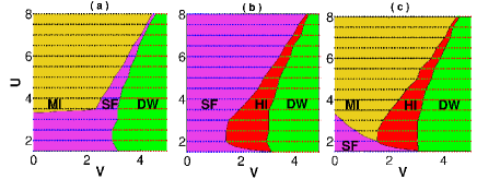
Figure 1: (Color online) Phase diagrams in the $(U,V)$ plane for the 1D EBHM with the following boundary conditions $(a)$ BC1 $(N=L)$, $(b)$ BC2 $(N=L+1)$, and $(c)$ BC3 $(N=L)$ and $\mu_{r}=-\mu_{l}=2$ showing Mott-insulator (MI ochre), superfluid (SF purple), Haldane-insulator (HI red), and density-wave (DW green) phases and the phase boundaries between them; in this range of $U$ and $V$ all transitions are continuous; at larger values of $U$ and $V$ the MI-DW and HI-DW transitions become first-order.

We now obtain the universality classes of the continuous transitions in the phase diagrams of Fig. 1. It has been noted in Ref. rvpai05 that the MI-SF transition in Fig. 1 (a), with BC1 boundary conditions, is in the Berezinskii-Kosterlitz-Thouless (BKT) class, whereas the SF-DW has both BKT and two-dimensional (2D) characters, in as much as the SF correlation length shows a BKT divergence but the DW order parameter decays to zero with a 2D-Ising, order-parameter exponent; this transition should be in the universality class of the Wess-Zumino-Witten $SU(2)_{1}$ theory like the critical point that lies between the BKT phase and the antiferromagnetic phase in the spin$-1/2$, XXZ antiferromagnetic chain shankar90 . The MI-SF and SF-DW phase boundaries in Fig. 1 (a) merge, most probably at a bicritical point, beyond which the MI-DW transition is first order rvpai05 . We concentrate here on the HI-SF, HI-DW, HI-MI transitions, all of which can be found in Fig. 1 (c), with the boundary condition BC3, for which we present results in Fig. 2; we have checked explicitly that the universality classes of the HI-SF and HI-DW transitions are the same with both BC2 and BC3 boundary conditions.

In Fig. 2 $(a_{1})$ we plot the scaled DW order parameter $O_{dw}L^{\beta/\nu}$ versus $V$ near the representative point, $V_{c}\simeq 3.86$ and $U=6$, on the HI-DW phase boundary for $L=200$ (red curve), $L=150$ (blue curve), and $L=100$ (green curve); the inset gives a plot of $O_{dw}L^{\beta/\nu}$ versus $(V-V_{c})^{\nu}L$; Fig. 2 $(a_{2})$ presents a similar plot and inset for the scaled structure factor $\mathcal{S}{({\pi})}L^{2\beta/\nu}$ at wave number $k=\pi$; in Fig. 2 $(a_{3})$ we plot the von-Neumann block entanglement entropy $S_{L}(l)$ versus the logarithmic conformal distance $\lambda$ for $L=220$ and a range of values of $V$ in the vicinity of $V_{c}(U=6)=3.86$. The values of the exponents $\beta$ and $\nu$ and the value of the central charge $c$ that we obtain from Figs. 2 $(a_{1})-(a_{3})$, namely, $\beta=1/8,\,\nu=1$, and $c=0.52$, are consistent with their values in 2D Ising model. If we restrict the occupancy to one boson per site, in the limit $U,V\to\infty$ with fixed $U/V$, the DW state can be represented as $|\dots 20202020\dots\rangle$ in the site-occupancy basis; this state is doubly degenerate and clearly breaks the translational symmetry of the lattice by doubling the unit cell; in contrast, the HI state has the translational invariance of the lattice. Given this double degeneracy of the DW state, we expect that, if the HI-DW transition is continuous, then it should be in the 2D Ising universality class; as we have shown above, our DMRG results for the HI-DW transition in the 1D EBHM are consistent with this expectation. Note that the string order parameter $O_{string}$ is nonzero in both the HI and DW phases; thus, it is not the order parameter that is required for identifying the universality class of the HI-DW transition. We find, furthermore, the string-order-parameter correlation length is so large in the HI phase that, given the values of $L$ in our study, it is not possible to get a reliable estimate for this correlation length.

To investigate the critical behavior of the MI-HI transition, we plot $R_{string}(k=0)L^{2\beta/\nu}$ versus $V$, in Fig. 2 $(b_{1})$, whose inset shows a plot of $R_{string}(k=0)L^{2\beta/\nu}$ versus $(V-{V_{c}})^{\nu}L$. These scaling plots indicate that, for $U=6$, the MI-HI critical point is at $V_{c}\simeq 3.5$ with exponents $\beta=0.35$ and $\nu=1.18$; this value of $\beta$ is consistent with the Gaussian-model gaussian1 (superscript $G$) result $\beta^{G}=1/\sqrt{8}$. Our value for $\nu$ follows from the plot of $L/\xi_{L}$ versus $V$ in Fig. 2 $(b_{2})$, whose inset shows a plot of $L/\xi_{l}$ versus $(V-{V_{c}})L^{1/\nu}$. For the central charge we obtain $c=1.02$, which is consistent with $c^{G}=1$ given our error bars, from the plot of $S_{L}(l)$ versus $\lambda$ for $L=220$ in Fig. 2 $(b_{3})$. As we have mentioned above, for large $U$ we can restrict the occupancies in the 1D EBHM to $0,\,1,$ and $2$ bosons per site to obtain a spin-1 model. The analog of the MI-HI transition in this spin-1 model has been shown to be in the Gaussian universality class gaussian1 , which has a fixed exponent $\beta=1/\sqrt{8}$ and central charge $c=1$, but an exponent $\nu$ that changes continuously along the phase boundary. We find indeed, from calculations like those presented in Figs. 2 $(b_{1})-(b_{3})$, that $\beta$ and $c$ do not change as we move along our MI-HI phase boundary in Fig. 1 (c), but $\nu$ does; we obtain, in particular, $\nu=1.18,\,1.22$, and $1.36$ for $U=6,\,5$, and $4$, respectively.

The critical behavior of the SF-HI transition follows from the plot of $R_{string}(k=0)L^{2\beta/\nu}$ versus $V$, in Fig. 2 $(c_{1})$, and the the plot of $L/\xi_{L}$ versus $V$, in Fig. 2 $(c_{2})$, whose inset shows a plot of $F$ versus $D$ (see Eq. 2). These scaling plots indicate that, for $V=0.9U$, the SF-HI critical point is at $V_{c}\simeq 1.7$, where the correlation length diverges with an essential singularity as it does at a BKT transition kogutreview . Thus, we cannot define the exponent $\nu$; however, we can define the exponent ratio $\beta/\nu$, which governs how rapidly the string order parameter vanishes as we approach the SF-HI phase boundary from the HI phase; for this ratio we obtain the estimate $\beta/\nu\simeq 0.9$. We find the central charge $c=0.94$, which is consistent with $c=1$ given our error bars, from the plot of $S_{L}(l)$ versus $\lambda$ for $L=280$ in Fig. 2 $(c_{3})$. The field theory for this SF-HI transition is likely to be non-standard because the SF phase has algebraic $U(1)$ order, whereas the HI phase has a non-local, string order parameter. An example of a similar transition is found in the phase diagram of the bilinear-biquadratic spin-1 chain, in which the Haldane phase (the analog of the HI phase here) undergoes a transition to a critical phase, as we change the ratio of the bilinear and biquadratic couplings; this transition is known to be described by an $SU(3)_{1}$ Wess-Zumino-Witten theory itoi . The gapless phase in our model is quite different from that in the spin-1 chain; and there is no $SU(3)$ symmetry at the SF-HI transition in the 1D EBHM. Nevertheless, it is likely that the SF-HI phase transition in our model is of a non-standard type, which is similar to, but not the same as, the $SU(3)_{1}$ theory mentioned above; this point requires more detailed investigations that lie beyond the scope of our paper. Note, furthermore, that the SF-HI transition here is not fine-tuned, unlike the one above in the spin-1 chain with bilinear and biquadratic couplings, in so far as the SF-HI transition occurs along an entire boundary in the phase diagram (Fig. 1 (c)).

For the sake of completeness we also show, for the BC3 boundary condition, the BKT nature of the SF-MI transition in Fig. 1 (c), as noted for the BC1 case in Ref. rvpai05 , by presenting plots of the scaled charge gap $F$ versus $D$ (see Eq. 2), the $k=0$ value of $n(k=0)$, and the block entanglement entropy $S_{L}(l)$ versus the log-conformal distance $\lambda$ in Figs. 2 $(d_{1})$, $(d_{2})$, and $(d_{3})$, respectively. These plots demonstrate that, at the MI-SF transition, the correlation length (or inverse charge gap) has a BKT-type essential singularity (Figs. 2 d₁), the SF-correlation-function exponent $\eta=1/4$, and the central charge is $c=0.96$, which is consistent with $c^{BKT}=1$ given our error bars. It is difficult to give precise error bars for the exponents and central charges that we have calculated because there are systematic errors, which include those associated with the finite values of $n_{max}$ and $n_{states}$; these errors are hard to estimate.

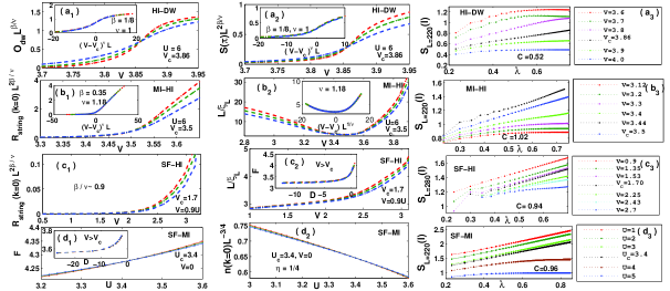
Figure 2: (Color online) Plots for the HI-DW transition at $U=6$, with $L=200$ (red curve), $L=150$ (green curve), and $L=100$ (blue curve), of $(a_{1})$ the scaled DW order parameter $O_{dw}L^{\beta/\nu}$ versus $V$ (the inset shows $O_{dw}L^{\beta/\nu}$ versus $(V-V_{c})^{\nu}L$), where $\beta$ and $\nu$ are order-parameter and correlation-length exponents, $(a_{2})$ the $k=\pi$ scaled structure factor $\mathcal{S}{({\pi})}L^{2\beta/\nu}$ versus $V$ (the inset shows $\mathcal{S}{({\pi})}L^{2\beta/\nu}$ versus $(V-V_{c})^{\nu}L$), and $(a_{3})$ the block entanglement entropy $S_{L}(l)$ versus the logarithmic conformal distance $\lambda={\frac{1}{6}}\log[\frac{2L}{\pi}\sin(\frac{\pi l}{L})]$ for an open system of length $L=220$ for different values of $V$ (the slope of the linear part of the curve for $V_{c}=3.86$ yields a central charge $c=0.52$). $(b_{1})$-$(b_{3})$ show the analogs, for the MI-HI transition, of the plots in $(a_{1})$-$(a_{3})$ but with $(b_{1})$ $O_{dw}L^{\beta/\nu}$ replaced by $R_{string}(k=0)L^{2\beta/\nu}$, the scaled Fourier transform of string correlation function at $k=0$, and $(b_{2})$ $\mathcal{S}{({\pi})}L^{2\beta/\nu}$ replaced by $L/\xi_{L}$; in ($b_{1}$) the values of $L$ are $290$ (red curve) $250$ (green curve), and $200$ (blue curve) and in ($b_{2}$) $L$ is $220$ (red curve) $200$ (green curve), and $180$ (blue curve). $(c_{1})$-$(c_{3})$ show the analogs, for the SF-HI transition, of the plots in $(b_{1})$-$(b_{3})$ (the inset in $(c_{2})$ shows a plot of the scaled charge gap $F$ versus $D$ (see Eq. 2)); in ($c_{1}$) and ($c_{2}$) the values of $L$ are $280$ (red curve) $240$ (green curve), and $200$ (blue curve). $(d_{1})$-$(d_{3})$ show the analogs, for the SF-MI transition, of the plots in $(b_{1})$-$(b_{3})$ but with $(d_{1})$ $R_{string}(k=0)L^{2\beta/\nu}$ replaced by the scaled charge gap $F$ and $V$ replaced by $U$ and $(d_{2})$ $L/\xi_{L}$ replaced by $n(k=0)L^{-3/4}$; in ($d_{1}$) $L$ is $200$ (red curve) $180$ (green curve), $160$ (blue curve) and in ($d_{2}$) $L$ is $250$ (red curve) $230$ (green curve), and $210$ (blue curve).

At lower values of $U$ and $V$ than those shown in Fig. 1, it has been suggested that the 1D EBHM can show a supersolid (SS) phase between SF and DW phases (see, e.g., Ref. deng12 ). However, it is not easy to distinguish such an SS phase from a region of first-order phase coexistence between SF and DW phases in a DMRG calculation, with a fixed number of bosons; we discuss this elsewhere tobepublished .

We have performed the most extensive DMRG study of the 1D EBHM attempted so far. Our work, which extends earlier studies rvpai05 ; entspect ; torre06 ; berg08 significantly, has been designed to investigate the effects of boundary conditions on the phase diagram of this model, to elucidate the natures of the phase transitions here, and to identify the universality classes of the continuous transitions. Our study shows that the HI-DW, MI-HI, and SF-MI transitions are, respectively, in the 2D Ising, Gaussian, and BKT universality classes; however, the SF-HI transition seems to be more exotic than a BKT transition in so far as the string order parameter also vanishes where the SF phase begins. We find that the different boundary conditions BC1, BC2, and BC3, which lead to the same value of $\rho$ in the thermodynamic limit, yield different phase diagrams; this boundary-condition dependence deserves more attention than it has received so far, especially from the point of view of the existence of thermodynamic limits thermodynamiclimit . We hope our work will stimulate more theoretical and experimental studies of the 1D EBHM and experimental realizations thereof.

We thank DST, UGC, CSIR (India) for support and E. Berg, E. G. Dalla Torre, F. Pollmann, E. Altman, A. Turner, and T. Mishra for useful discussions.

References

- (1) I. Bloch, J. Dalibard, and W. Zwerger, Rev. Mod. Phys. 80, 885 (2008); M. Lewenstein, A. Sanpera, V. Ahufinger, B. Damski, A. Sen(De) and U. Sen, Adv. in Physics, 56 243 (2007).
- (2) M.P.A. Fisher, P.B. Weichman ,G. Grinstein and D.S. Fisher, Phys. Rev. B 40, 546 (1989).
- (3) K. Sheshadri, H. R. Krishnamurthy, R. Pandit and T. V. Ramakrishnan, Europhys. Lett. 22 257 (1993).
- (4) D. Jaksch, C. Bruder, J. I. Cirac, C. W. Gardiner and P. Zoller, Phys. Rev. Lett. 81, 3108 (1998); M. Greiner, O. Mandel, T. Esslinger, T.W. Hänsch and I. Bloch, Nature (London) 415, 39 (2002).
- (5) T. Kühner and H. Monien, Phys. Rev. B 58, R14741 (1998).
- (6) R.V. Pai and R. Pandit , Phys. Rev. B, 71, 104508 (2005); Proceedings of the Indian Academy of Sciences (Chemical Science) 115, Nos. 5-6, 721 (2003).
- (7) X. Deng and L. Santos , Phys. Rev. B 84, 085138 (2011).
- (8) J.M. Kurdestany, R.V. Pai, and R. Pandit, Ann. Phys. (Berlin) 524 No. 3-4, 234 (2012).
- (9) E.G. Dalla Torre, E. Berg, and E. Altman, Phys. Rev. Lett. 97, 260401 (2006).
- (10) E. Berg, E.G. Dalla Torre, T. Giamarchi, and E. Altman, Phys. Rev. B, 77, 245119 (2008).
- (11) D. Kovrizhin, G.V. Pai, and S. Sinha, Europhys. Lett. 72, 162 (2005); A.F. Andreev and I.M. Lifshitz, Sov. Phys. JETP, 29, 1107 (1969); A.J. Leggett, Phys. Rev. Lett. 25, 1543 (1970); G. Chester, Phys. Rev. A 2, 256 (1970); E. Kim and M.H.W. Chan, Nature 427, 225 (2004).
- (12) J. Werner, A. Griesmaier, S. Hensler, J. Stuhler, and T. Pfau, Phys. Rev. Lett. 94, 183201 (2005).
- (13) K. Göral, L. Santos and M. Lewenstein, Phys. Rev. Lett. 88, 170406 (2002).
- (14) X. Deng, R. Citro, E. Orignac, A. Minguzzi, and L. Santos (2012) arXiv:1203.0505v1.
- (15) D. Rossini and R. Fazio, New Journal of Physics 14, 065012 (2012).
- (16) D. Ruelle, Statistical Mechanics: Rigorous Results (Imperial College Press and World Scientific, London and Singapore, 1999); O. Bratelli and D.W. Robinson, Operator Algebras and Quantum Statistical Mechanics 2 (Springer Verlag, Berlin, 2002).
- (17) J.B. Kogut, Rev. Mod. Phys. 51, 4 (1979).
- (18) S. Hu, B. Normand, X. Wang and L. Yu, Phys. Rev. B 84, 220402(R)(2011).
- (19) We use the conventional terminology charge gap even though we do not have charged bosons in mind. Indeed, some authors refer to our DW phase as a CDW phase.
- (20) Andreas M. L\a”uchli and C. Kollath, J. Stat. Mech. 2008 P05018.
- (21) R. Shankar and N. Read, Nucl. Phys. B 336, 457 (1990).
- (22) C. Itoi and M-H. Kato, Phys. Rev. B 55, 8295 (1997).
- (23) J.M. Kurdestany, R.V. Pai, S. Mukerjee, and R. Pandit, to be published.