Non-linear Coulomb blockade microscopy of a correlated one-dimensional quantum dot

Abstract

We evaluate the chemical potential of a one-dimensional quantum dot, coupled to an atomic force microscope tip. The dot is described within the Luttinger liquid framework and the conductance peaks positions as a function of the tip location are calculated in the linear and non-linear transport regimes for an arbitrary number of particles. The differences between the chemical potential oscillations induced by Friedel and Wigner terms are carefully analyzed in the whole range of interaction strength. It is shown that Friedel oscillations, differently from the Wigner ones, are sensitive probes to detect excited spin states and collective spin density waves involved in the transport.

When electrons are confined in a finite portion of condensed matter, such as in quantum dots [1], many intriguing physical effects appear. Quantum confinement induces Friedel oscillations [2] in the electron density with a typical wavelength $(2k_{F})^{-1}$ ($k_{F}$ the Fermi momentum). In addition, when the Coulomb repulsion dominates over the kinetic energy, electrons tend to form a Wigner crystal [3, 4] giving rise to density oscillations at wavelength $(4k_{F})^{-1}$. In two-dimensional dots, correlation effects have been extensively studied mainly by means of numerical techniques [3, 4, 5, 6, 7]. Due to the reduced dimensionality, one-dimensional (1D) quantum dots, such as carbon nanotubes [8], show even more dramatic interaction effects. They have been indeed the subject of intense numerical investigations [9, 10, 11, 12, 13, 14]. Despite their precision, numerical methods are usually restricted to a low number of particles due to their complexity. An analytical approach, widely employed to describe the physics of interacting 1D electrons, is the Luttinger liquid model [15, 16, 17, 18, 19]. In connection with the bosonization technique, it represents a powerful method to study the low-energy physics, allowing to explore the limit of large particle numbers and addressing their transport properties [20, 21, 22, 23, 24] and the formation of Wigner crystals [25, 26, 27, 28, 29].

One of the key tools to investigate the emergence of Friedel and Wigner correlations is exploiting the dot transport properties in the presence of a local probe. Scanning tunnel microscope tips have been proposed in the past to detect Friedel [30, 31, 32] or Wigner oscillations [33] and even local electron-vibron coupling [34]. The most natural and powerful choice is however that of an atomic force microscope (AFM) tip which capacitively couples to the dot density and thus allows to capture its oscillations, a technique called ”Scanning gate microscopy” [35, 36]. Recent theoretical studies [13, 37] have investigated the influence of an AFM tip on the dot chemical potential revealing its spatial oscillations as a function of the tip position. These works, however, have only considered the linear regime, allowing to access only the ground state properties of systems with low electrons numbers [13].

In this paper we will go beyond these limitations. Employing the Luttinger liquid and the bosonization language [16, 18, 25, 38, 39] we will develop a fully analytical framework which will enable us to study the position of the conductance peaks in the presence of a moving AFM tip, both in the linear and in the non-linear regime. To this end, we will evaluate the chemical potential traces as a function of the tip position and electron interaction strength, without any limitation on the electron number. We will show that Friedel and Wigner oscillations produce different signatures due to the spin dynamics, demonstrating that Friedel correlations are sensitive to the spin populations of electrons in the quantum dot. In the non-linear case, where higher excited spin are involved, Friedel oscillations increase their number, reaching the one of the Wigner case for a fully polarized dot. Also collective spin density excitations induce additional density modulations which can as well be detected in the chemical potential traces.

We consider an interacting 1D quantum dot, treated as a Luttinger liquid with open boundaries. The reference state is set with an even electron number $N^{0}$ and Fermi momentum $k_{F}=\pi N^{0}/2L$ ($L$ dot length). The low energy Hamiltonian takes the form [18] ($\hbar=1$)

$$H_{d}=\sum_{\nu=\rho,\sigma}\sum_{q>0}\varepsilon_{\nu}(q)d^{\dagger}_{\nu,q}d_{\nu,q}+\frac{E_{\rho}}{2}\Delta N_{\rho}^{2}+\frac{E_{\sigma}}{2}\Delta N_{\sigma}^{2}\,.$$ (1)

Here, $d_{\nu,q}$ are the boson operators of the collective charge ($\nu=\rho$) and spin ($\nu=\sigma$) density waves, with quantized wave number $q=\pi n_{q}/L$, $n_{q}\in\mathbb{N}^{*}$ and energy $\varepsilon_{\nu}(q)=\varepsilon_{\nu}n_{q}$, where $\varepsilon_{\nu}=\pi v_{\nu}/L$. They propagate at a renormalized velocity $v_{\nu}=v_{F}/g_{\nu}$, ($v_{F}$ the Fermi velocity) without a change in the total number of charges and spin. The repulsive electron interaction strength is represented by $g_{\rho}=g<1$, while $g_{\sigma}=1$ for an SU(2) invariant theory [16]. The second part of the Hamiltonian represents the zero mode contributions with $\Delta N_{\rho,\sigma}=\Delta N_{+}\pm\Delta N_{-}$, where $\Delta N_{s}=N_{s}-N_{s}^{0}$ are the extra electrons per spin direction ($s=\pm$) with respect to the reference $N_{+}^{0}=N_{-}^{0}=N^{0}/2$. The total charge and spin are $N_{\rho}=\Delta N_{\rho}+N_{0}$ and $N_{\sigma}=\Delta N_{\sigma}$, with energies $E_{\rho}$ and $E_{\sigma}$. Despite the microscopic model provides their quantitative estimates ($E_{\nu}=\pi v_{\nu}/2Lg_{\nu}$), several effects, e.g. coupling with the external gates or long range interactions, cause deviations especially in the charge sector. Therefore, we treat $E_{\rho}$ as a free parameter, with $E_{\rho}\gg E_{\sigma}$, while keeping $E_{\sigma}=\pi v_{F}/2L=\varepsilon_{\sigma}/2$.

Let us denote the eigenstates of the above Hamiltonian as $|\mathcal{S}\rangle\equiv|N_{\rho},N_{\sigma},\{n_{q}^{\rho}\},\{n_{q}^{\sigma}\}\rangle$ with energies

$$E(\mathcal{S})=\sum_{\nu=\rho,\sigma}\left[\frac{E_{\nu}}{2}\Delta N_{\nu}^{2}+\sum_{q>0}\varepsilon_{\nu}n_{q}^{\nu}\right]\,,$$ (2)

where $\{n_{q}^{\nu}\}$ are the occupation numbers for the collective mode $\nu$ at momentum $q$.

The electron operator $\Psi_{s}(x)$, with boundary conditions $\Psi_{s}(0)=\Psi_{s}(L)=0$, is represented in terms of right-moving electrons as $\Psi_{s}(x)=e^{ik_{F}x}\psi_{s,R}(x)-e^{-ik_{F}x}\psi_{s,R}(-x)$ [18]. In bosonized form,

$$\psi_{s,R}(x)=\frac{\eta_{s}}{\sqrt{2\pi\alpha}}e^{-i\theta_{s}}\,e^{i\frac{\pi\Delta N_{s}x}{L}}e^{i\frac{\Phi_{\rho}(x)+s\Phi_{\sigma}(x)}{\sqrt{2}}}\,.$$ (3)

Here, $\{\eta_{s},\eta_{s^{\prime}}\}=\delta_{s,s^{\prime}}$, $\alpha=k_{F}^{-1}$ the cutoff length, $[\theta_{s},\Delta N_{s^{\prime}}]=i\delta_{s,s^{\prime}}$ and

$$\Phi_{\nu}(x)\!=\!\sum_{q>0}\frac{e^{-\alpha q/2}}{\sqrt{g_{\nu}n_{q}}}\left[\left(\cos{(qx)}-ig_{\nu}\sin{(qx)}\right)d^{\dagger}_{\nu,q}\!+\mathrm{h.c.}\right].$$

The total electron density $\rho(x)=\sum_{s}\rho_{s}(x)$ with $\rho_{s}(x)=\Psi_{s}^{\dagger}(x)\Psi_{s}(x)$ consists of several contributions [25, 28]. Here we take into account the most relevant adopting a number-conserving formalism [29] for open boundaries. The smooth long-wave term $\rho^{LW}(x)=\sum_{s}\rho_{s}^{LW}(x)$ is given by

$${\rho}_{s}^{LW}(x)=\frac{k_{F}}{\pi}+\frac{\Delta N_{s}}{L}+\frac{1}{\pi}\partial_{x}\varphi_{s}(x)-\frac{g^{2}}{\pi}\partial_{x}h(x)\,,$$ (4)

with $\varphi_{s}(x)=\left[\varphi_{\rho}(x)+s\varphi_{\sigma}(x)\right]/\sqrt{2}$ where

$$\varphi_{\nu}(x)=\frac{1}{2}\left[\Phi_{\nu}(x)-\Phi_{\nu}(-x)\right]$$ (5)

and $h(x)=\frac{1}{2}\tan^{-1}\left[\frac{\sin(2\pi x/L)}{e^{\pi\alpha/L}-\cos(2\pi x/L)}\right]$.

The oscillating Friedel contribution is $\rho^{F}(x)\propto\sum_{s}\rho^{F}_{s}(x)$ with $\rho^{F}_{x}(x)=e^{-2ik_{F}x}\psi_{s,R}^{\dagger}(x)\psi_{s,R}(-x)+\mathrm{h.c.}$. In bosonic representation one has

$${\rho}^{F}_{s}(x)=-\frac{1}{2\pi}\partial_{x}\sin\left[\mathcal{L}(\Delta N_{s},x,g)+2\varphi_{s}(x)\right]\,,$$ (6)

where

$$\mathcal{L}(n,x,g)=2k_{F}x+\frac{2\pi nx}{L}-2g^{2}h(x)\,.$$ (7)

In addition to these “standard” terms we include the so-called Wigner contribution $\rho^{W}(x)\propto e^{-4ik_{F}x}\psi_{+,R}^{\dagger}(x)\psi_{+,R}(-x)\psi_{-,R}^{\dagger}(x)\psi_{-,R}(-x)+\mathrm{h.c.}$ which may arise due to interaction effects, band curvature or other external perturbations [26, 28, 27]. In the bosonization language [25] one has

$$\rho^{W}(x)=-\frac{1}{2\pi}\partial_{x}\sin\left[2\mathcal{L}\left(\frac{\Delta N_{\rho}}{2},x,g\right)+2\sqrt{2}\varphi_{\rho}(x)\right]\,.$$ (8)

Note that these terms constitute the most relevant contributions to the electron density, whose amplitudes are to be interpreted as model parameters [25, 28]. The total density, satisfying boundary conditions $\rho(0)=\rho(L)=0$, can then be expressed as

$$\rho(x)=\rho^{LW}(x)+(1-\lambda)\rho^{F}(x)+\lambda\rho^{W}(x)\,,$$ (9)

with $\lambda\in[0,1]$ a free parameter.

We now analyze the expectation values ${\rho}_{GS}^{\xi}(x)=\langle\mathcal{S}|\rho^{\xi}(x)|\mathcal{S}\rangle_{GS}$ on the ground state $|\mathcal{S}\rangle_{GS}=|N_{\rho}^{GS},{N}_{\sigma}^{GS},\{n_{q}^{\rho}=0\},\{n_{q}^{\sigma}=0\}\rangle$ for the different contributions $\xi=LW,F,W$. Note that, due to $N^{0}$ being even, one has $N_{\rho}^{GS}=N^{0}$ and $N_{\sigma}^{GS}=0$ with $\Delta N_{\nu}^{GS}=0$ for an even number of electrons, while $N_{\rho}^{GS}=N^{0}+1$ and ${N}_{\sigma}^{GS}=\pm 1$ with $\Delta N_{\rho}^{GS}=1$ for the nearest larger odd electron number. Using the bosonization technique one obtains

$$\!\!\rho_{GS}^{LW}(x) = \frac{2k_{F}}{\pi}+\frac{\Delta N_{\rho}^{GS}}{L}-2\frac{g^{2}}{\pi}\partial_{x}h(x)\,,$$ (10)

$$\!\!\rho_{GS}^{F}(x) = \!-\frac{1}{2\pi}\partial_{x}\!\!\left\{\!\!K^{F}\!\sum_{s=\pm}\sin\left[\mathcal{L}(\Delta N_{s}^{GS},x,g)\right]\right\},$$ (11)

$$\!\!\rho_{GS}^{W}(x) = \!-\frac{1}{2\pi}\partial_{x}\!\!\left\{\!\!K^{W}\!\sin\left[2\mathcal{L}\left(\frac{\Delta N_{\rho}^{GS}}{2},x,g\right)\right]\right\}$$ (12)

with the enveloping functions ($\eta_{F}=\frac{1+g}{2}$; $\eta_{W}=2g$)

$$K^{\xi}(x)=\left[\frac{\sinh\left({\frac{\pi\alpha}{2L}}\right)}{\sqrt{\sinh^{2}\left({\frac{\pi\alpha}{2L}}\right)+\sin^{2}\left(\frac{\pi x}{L}\right)}}\right]^{\eta_{\xi}}\,.$$ (13)

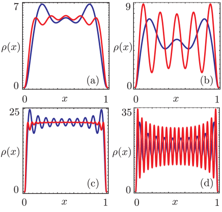
Figure 1: Ground state dot electron density (units $L^{-1}$) as a function of $x$ (units $L)$ for (a) $N_{\rho}^{GS}=5$, $g=0.9$; (b) $N_{\rho}^{GS}=5$, $g=0.1$; (c) $N_{\rho}^{GS}=20$, $g=0.9$; (d) $N_{\rho}^{GS}=20$, $g=0.1$. The blue (red) curve represents the Friedel (Wigner) contributions in addition to the long-wave part. In (a,b) $\alpha^{-1}=2\pi/L$, in (c,d) $\alpha^{-1}=10\pi/L$.

Let us now study the Friedel and Wigner contributions separately. Figure 1 shows the electron density, see Eq. (9), in the ground state with the long wave part and the Friedel ($\lambda=0$) or the Wigner ($\lambda=1$) terms. In both cases it exhibits an oscillatory behaviour but with different patterns and amplitudes. The Friedel contribution shows oscillations related to the two different electron spin populations. In particular, for even electrons one has $N_{s}^{GS}=N_{\rho}^{GS}/2$ and thus the superposition results in $N_{\rho}^{GS}/2$ peaks. For odd numbers, one of the two subpopulations has $(N_{\rho}^{GS}+1)/2$ electrons, while the other has $(N_{\rho}^{GS}-1)/2$. The superposition for both spin directions has then $(N^{GS}_{\rho}+1)/2$ peaks. The Wigner correction, on the other hand, is insensitive to spin, see Eq. (12), and depends on $N^{GS}_{\rho}$ only, which is also the number of observed peaks.

Concerning amplitudes one can easily see that Friedel oscillations are dominant over the Wigner ones for weak interactions, Panels (a,c), while for strong interactions, Panels (b,d), the situation is reversed. This fact is particularly evident when the number of particles increases.

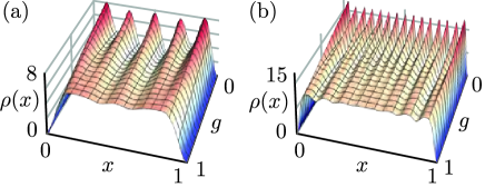
Figure 2: Ground state electron density (units $L^{-1}$) as a function of $x$ (units $L$) and $g$ for $\lambda=0.5$. (a) $N^{GS}_{\rho}=5$ and $\alpha^{-1}=2\pi/L$; (b) $N^{GS}_{\rho}=15$ and $\alpha^{-1}=7\pi/L$.

Let us now consider the combined effects of both contributions. Figure 2 shows $\rho_{GS}(x)$ as a function of $x$ and $g$ for $\lambda=0.5$, see Eq. (9). For weak interactions ($g\approx 1$) one can distinguish $(N^{GS}_{\rho}+1)/2$ peaks (in both panels $N^{GS}_{\rho}$ is odd). At strong interactions ($g\to 0$), Wigner correlations grow and eventually the density exhibits sharp oscillations with $N^{GS}_{\rho}$ peaks. Thus, even when Wigner correlations are mixed along with Friedel ones, the presence of strong interactions makes the Wigner channel the relevant one. The above behaviour can be attributed to the enveloping functions $K^{F}(x)$ and $K^{W}(x)$ in Eq. (13). For $g\to 1$, the weaker power law in $K^{F}(x)$ (namely, $x^{-(1+g)/2}$) in comparison to that of $K^{W}(x)$ (namely, $x^{-2g}$) leads to a suppression of the Wigner channel. On the other hand, when $g\to 0$ one has $K^{W}(x)\to 1$ and $K^{F}(x)\ll 1$ away from the borders. Thus, for strong interactions Friedel oscillations are damped, while the Wigner ones are still fully developed.

We would like now to show how to probe electron density correlations in the presence of a movable AFM tip. This has already been considered as a powerful tool to investigate the electronic correlated state for linear transport in dots with few electrons [13]. Here, we will consider the more general non-linear regime, without any constraint on the number of electrons.

The charged AFM tip is capacitively coupled to the dot at position $x$, with coupling $H_{tip}=V_{0}\rho(x)$, assuming a tip narrower than the average wavelength of the density oscillations. In the sequential regime, for a given transition $|\mathcal{S}\rangle\to|\mathcal{S}^{\prime}\rangle$ electrons tunnel between the dot and the leads and the number of dot charges oscillates between $N_{\rho}$ and $N_{\rho}+1$, with the spin constraint $|N^{\prime}_{\sigma}-N_{\sigma}|=1$. The onset of a transition is signalled by peaks in the differential conductance. In the following we will determine their positions as a function of the tip. The key quantity to evaluate is the generalized chemical potential

$$\mu_{\mathcal{S}\to\mathcal{S}^{\prime}}(x)=E_{tot}(\mathcal{S}^{\prime},x)-E_{tot}(\mathcal{S},x)\,,$$ (14)

defined in terms of the total energy $E_{tot}(\mathcal{S},x)$ in the presence of the tip. Indeed, whenever $\mu_{\mathcal{S}\to\mathcal{S}^{\prime}}(x)\approx\mu_{\chi}$, where $\mu_{\chi}$ is the electrochemical potential of the lead $\chi$ the given transition becomes allowed. We will evaluate Eq. (14) in the weak tip-coupling regime, namely $E_{tot}(\mathcal{S},x)=E(\mathcal{S})+\delta E(\mathcal{S},x)$ with $\delta E(\mathcal{S},x)$ the lowest order correction.

We will consider only non-degenerate energy levels, whose corrections to the energy $E(\mathcal{S})$ in Eq. (2) are given by $\delta E(\mathcal{S},x)=V_{0}\langle\mathcal{S}|\rho(x)|\mathcal{S}\rangle$. This is a relevant case since it applies to zero-mode spin excited states (the degeneracy on $\pm|N_{\sigma}|$ is explicitly diagonal and does not cause problems) and to the lowest lying spin density waves with a singly occupied bosonic state. The latter is indeed non degenerate in the presence of interactions since $\varepsilon_{\sigma}<\varepsilon_{\rho}$. Generalizing the results obtained for the ground state one has $\delta E(\mathcal{S},x)\!=\!\delta E^{LW}(\mathcal{S},x)+(1-\lambda)\delta E^{F}(\mathcal{S},x)+\lambda\delta E^{W}(\mathcal{S},x)$, with

$$\delta E^{LW}(\mathcal{S},x)\!=\!V_{0}\left[\frac{2k_{F}}{\pi}+\frac{\Delta N_{\rho}}{L}-2\frac{g^{2}}{\pi}\partial_{x}h(x)\right]$$ (15)

$$\delta E^{F}(\mathcal{S},x)\!=\!-\frac{V_{0}}{2\pi}\!\partial_{x}\!\!\left(\!K^{F}\!G^{F}\sum_{s=\pm}\sin\left[\mathcal{L}(\Delta N_{s},x,g)\right]\right)$$ (16)

$$\delta E^{W}(\mathcal{S},x)\!=\!-\frac{V_{0}}{2\pi}\!\partial_{x}\!\!\left(\!\!K^{W}\!G^{W}\!\!\sin\left[2\mathcal{L}\left(\!\frac{\Delta N_{\rho}}{2},x,g\right)\right]\right)$$ (17)

Here we introduced $G^{F}(x)=\prod_{\nu}\prod_{q>0}L_{n_{q}^{\nu}}\left[A_{q}^{\nu}(x)^{2}\right]$ and $G^{W}(x)=\prod_{q>0}L_{n_{q}^{\rho}}\left[A_{q}^{\rho}(x)^{2}\right]$, with $L_{n}(x)$ the Laguerre polynomials stemming from generalized Franck-Condon factors [40, 41] and $A_{q}^{\nu}(x)=\sqrt{\frac{2\pi g_{\nu}}{qL}}e^{-\alpha q/2}\sin(qx)$. In the absence of collective modes one has $G^{F}(x)=G^{W}(x)=1$.

The corresponding chemical potential is then decomposed as the bare one, $\mu_{0,\mathcal{S}\to\mathcal{S}^{\prime}}=E(\mathcal{S^{\prime}})-E(\mathcal{S})$ - see Eq. (2) - and the tip correction, $\delta\mu_{\mathcal{S}\to\mathcal{S}^{\prime}}(x)=\delta E(\mathcal{S}^{\prime},x)-\delta E(\mathcal{S},x)$ - see Eqs. (15-17). In short notation, omitting the states, one has

$$\mu(x) = \mu_{0}+\delta\mu(x)$$ (18)

$$\delta\mu(x) = \delta\mu^{LW}+(1-\lambda)\delta\mu^{F}(x)+\lambda\delta\mu^{W}(x)\,.$$ (19)

We are now in the position to investigate the chemical potential variation as a function of the tip position for a given transition. We start by considering the linear regime where only the ground states are involved: $|\mathcal{S}\rangle_{GS}$ with total number $N_{\rho}$ and $2|{N}_{\sigma}|=1-(-1)^{N_{\rho}}$, and $|\mathcal{S}^{\prime}\rangle_{GS}$ with $N^{\prime}_{\rho}=N_{\rho}+1$ and $2|{N}^{\prime}_{\sigma}|=1-(-1)^{N^{\prime}_{\rho}}$.

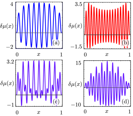
Figure 3: Chemical potential corrections $\delta\mu(x)$ (units $V_{0}/L$) in the linear regime as a function of $x$ (units $L$) for the transition with $N_{\rho}=16$. (a) Friedel corrections only ($\lambda=0$) and $g=0.7$ ; (b) same as in (a) but for Wigner ($\lambda=1$); (c) same as in (a) but with Friedel and Wigner ($\lambda=1/2$); (d) same as in (c) but for stronger interactions $g=0.1$. In all panels, $\alpha^{-1}=8\pi/L$.

Figure 3 shows the correction $\delta\mu(x)$ in Eq. (19). One can observe sharp oscillations, induced by the difference of two oscillating quantities and in contrast to the weaker ones displayed in the electron density. The Friedel term, shown in Panel (a) for even $N_{\rho}$ and $N_{\sigma}=0$, displays $1+N_{\rho}/2$ maxima and $N_{\rho}/2$ minima. The number of these maxima is related to the spin population of the dot final state. Indeed, the initial spin populations are $N_{s}=N_{\rho}/2$. When an extra electron, with spin up, enters into the dot, the state with $N^{\prime}_{\sigma}=1$ is reached with $N^{\prime}_{+}=1+N_{\rho}/2$ and $N^{\prime}_{-}=N_{\rho}/2$. These are indeed the values which correspond to the number of maxima and minima exhibited. A similar behaviour holds for an odd number $N_{\rho}$ (not shown) where one finds $(N_{\rho}+1)/2$ maxima and $(N_{\rho}-1)/2$ minima. Thus, in the Friedel case the oscillations of the chemical potential are a sensitive probe to detect the spin sub-populations of the electron involved in the linear transport process. The Wigner case, on the other hand, is not sensitive to the spin direction. As shown in Panel (b), it always displays $N_{\rho}+1$ maxima and $N_{\rho}$ minima, allowing to count the total number of electrons only. Panels (c,d) show the combined effect of equally weighted Friedel and Wigner corrections. For strong interactions, Panel (d), Wigner corrections are clearly well pronounced, differently from the weak interactions case, Panel (c). These results are in agreement with the ones obtained for few particles with an exact diagonalization procedure [13] .

Let us turn to the non-linear case, with excited zero mode spin states and for the moment without collective modes. This has never been investigated in literature to our knowledge. The transitions are between states of the form $|\mathcal{S}\rangle=|N_{\rho},N_{\sigma}\rangle$ and $|\mathcal{S}^{\prime}\rangle=|N_{\rho}+1,N^{\prime}_{\sigma}\rangle$, with $N_{\sigma}$, $N^{\prime}_{\sigma}$ not restricted to the ground state values anymore. We select, in particular $N^{\prime}_{\sigma}=N_{\sigma}+1$ and $N_{\rho}=2\kappa$ with $\kappa\in\mathbb{N}^{*}$, focusing on the Friedel contribution only. The Wigner one is indeed insensitive to the total spin - see Eq. (17) - and will give, for each of the above transitions, a contribution equal to that of the linear case. The possible spin transitions are $|N_{\rho},0\rangle\to|N_{\rho}+1,1\rangle$; $|N_{\rho}+1,1\rangle\to|N_{\rho},2\rangle$; $\cdots;|N_{\rho},N_{\rho}\rangle\to|N_{\rho}+1,N_{\rho}+1\rangle$. Namely, the dot starts in the ground state with $N_{s}=N_{\rho}/2$, eventually becoming fully polarized.

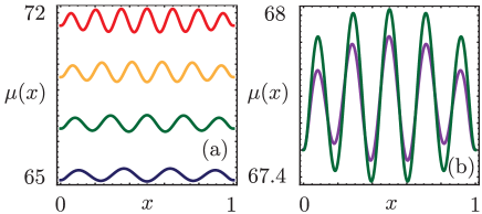
Figure 4: Chemical potential $\mu(x)$ (units $E_{\sigma}$) as a function of $x$ (units $L$) including only the Friedel corrections. (a) Traces of the transition $|6,0\rangle\to|7,1\rangle$ (blue), $|6,2\rangle\to|7,3\rangle$ (green), $|6,4\rangle\to|7,5\rangle$ (orange), $|6,6\rangle\to|7,7\rangle$ (red); (b) Traces for a transition $|6,0,\{n_{q}^{\rho}=0\},\{n_{q}^{\sigma}=0\}\rangle\to|7,1,\{n_{q}^{\rho}=0\},\{n_{q}^{\sigma}=\delta_{q,\pi/L}\}\rangle$ involving a spin density wave (black) and $|6,2\rangle\to|7,3\rangle$ involving zero-modes only (green). In all panels $g=0.7$, $E_{\rho}=10E_{\sigma}$, $V_{0}=0.08E_{\sigma}$ and $\alpha^{-1}=3\pi/L$.

As a representive example we show in Fig. 4(a) the position dependence of the chemical potential in Eq. (18) with the Friedel contribution for the tunnel-in transitions. Starting with $N_{\rho}/2+1$ maxima in the ground states (blue trace), an increasing number of oscillations appear as higher spin states get involved. Eventually, the transition involving fully polarized dot state is reached and the chemical potential shows with $N_{\rho}+1$ maxima (red trace). Note that this is the same number of maxima that one would obtain from the Wigner corrections.

The sensitivity of the Friedel corrections to spin suggests to employ non-linear transport experiments in the presence of an AFM tip to explore highly excited spin states of quantum dots. This seems particularly desirable for not too strong interactions, when the Wigner corrections do not dominate over the Friedel ones. It is also possible to conclude that the observation of $N_{\rho}+1$ peaks in the chemical potential for an excited transition does not provide alone a clear-cut evidence of the presence of Wigner correlations.

We close our discussion briefly addressing how the above effect can be obtained also for transitions involving excited spin density waves previously neglected. In general, and in contrast to zero-mode excitations, collective modes are assumed to relax to the ground state over a time shorter than the average tunneling time of electrons due to several possible types of dissipative coupling. This implies excitations only in final states. To be more specific we consider a transition from the ground state to the lowest-lying collective spin excitation with $q=\pi/L$. The two involved states are $|N_{\rho},0,\{0\}_{\rho},\{0\}_{\sigma}\rangle\to|N_{\rho}+1,1,\{0\}_{\rho},\{n_{q}^{\sigma}=\delta_{q,\pi/L}\}\rangle$ with $N_{\rho}$ even. Figure 4(b) shows the corresponding chemical potential with Friedel corrections for $N_{\rho}=6$. It exhibits five peaks and the overall behaviour is similar to the green trace in Fig. 4(a) corresponding to $|6,2\rangle\to|7,3\rangle$. Indeed since $2E_{\sigma}=\varepsilon_{\sigma}$ the two transitions have the same bare chemical potential $\mu_{0}=E_{\rho}\left(2N_{\rho}+1\right)/{2}+5E_{\sigma}/{2}$ but different corrections $\delta\mu(x)$ also due to the different contribution of the function $G^{F}(x)$ in Eq. (16).

In conclusion, we have studied the chemical potential traces of an interacting 1D quantum dot in the presence of a coupling with a moving AFM tip. As a general trend, we have found that Friedel modulations dominate for weak interactions and are sensitive to spin populations, while the Wigner oscillations become relevant at strong interactions and depend on the total charge sector only. We demonstrated that this results in markedly different behaviours. In the linear regime, Friedel correlations exhibit half of the number of oscillations than the Wigner ones. On the other hand, in the non-linear case, when higher excited spin are involved, they increase the number of oscillations, reaching the one of the Wigner case for a fully polarized dot. We expect that predicted oscillations of the chemical potential traces as a function of the AFM tip can be observed in transport experiments.

Acknowledgements. Financial support by the EU-FP7 via ITN-2008-234970 NANOCTM is gratefully acknowledged.

References

- [1] Kouwenhoven L and Marcus C 1998 Physics World June 35
- [2] Giuliani F G and Vignale G 2005 Quantum Theory of the Electron Liquid (Cambridge University Press)
- [3] Reimann S M and Manninen M 2002 Rev. Mod. Phys. 74 1283
- [4] Yannouleas C and Landman U 2007 Rep. Prog. Phys. 70 2067
- [5] Egger R, Häusler W, Mak C H and Grabert H 1999 Phys. Rev. Lett. 82 3320
- [6] Rontani M, Molinari E, Maruccio G, Janson M, Schramm M, Meyer C, Matsui T, Heyn C, Hansen W and Wiesendanger R 2007 J. Appl. Phys. 101 081714
- [7] Cavaliere F, De Giovannini U, Sassetti M and Kramer B 2009 New J. Phys. 11 123004
- [8] Bockrath M, Cobden D H, McEuen P L, Chopra N G, Zettl A, Thess A and Smalley R E 1997 Science 275 1922
- [9] Häusler W and Kramer B 1993 Phys. Rev. B 47 16353
- [10] Agosti D, Pederiva F, Lipparini E and Takayanagi K 1998 Phys. Rev. B 57 14869
- [11] Abedinpour S H, Polini M, Xianlong G and Tosi M P 2007 Phys. Rev. A 75 015602
- [12] Secchi A and Rontani M 2009 Phys. Rev. B 80 041404(R)
- [13] Qian J, Halperin B I and Heller E J 2010 Phys. Rev. B 81 125323
- [14] Astrakharchik G E and Girardeau M D 2011 Phys. Rev. B 83 153303
- [15] Haldane F D 1981 Phys. Rev. Lett. 47 1840
- [16] Voit J 1995 Rep. Prog. Phys. 58 977
- [17] Giamarchi T 2004 Quantum Physics in One Dimension (Oxford Science Publications)
- [18] Fabrizio M and Gogolin A O 1995 Phys. Rev. B 51 17827
- [19] Cuniberti G, Sassetti M and Kramer B 1998 Phys. Rev. B 57 1515; Sassetti M and Kramer B 1998 Phys. Rev. Lett. 80 1485
- [20] Egger R and Grabert H 1997 Phys. Rev. Lett. 79 3463
- [21] Kleimann T, Cavaliere F, Sassetti M and Kramer B 2002 Phys. Rev. B 66 165311; Parodi D, Sassetti M, Solinas P, Zanardi P and Zanghì N 2006 Phys. Rev. A 73 052304
- [22] Cavaliere F, Braggio A, Stockburger J T, Sassetti M and Kramer B 2004 Phys. Rev. Lett. 93 036803
- [23] Mayrhofer L and Grifoni M 2007 Eur. Phys. J. B 56 107
- [24] Grifoni M, Sassetti M and Weiss U 1996 Phys. Rev. E 53 R2033; Ferraro D, Braggio A, Magnoli N and Sassetti M 2010 Phys. Rev. B 82 085323
- [25] Schulz H J 1993 Phys. Rev. Lett. 71 1864
- [26] Safi I and Schulz H J 1999 Phys. Rev. B 59 3040
- [27] Fiete G A, Le Hur K and Balents L 2006 Phys. Rev. B 73 165104
- [28] Söffing S A, Bortz M, Schneider I, Struck A, Fleischhauer M and Eggert S 2009 Phys. Rev. B 79 195114
- [29] Gindikin Y and Sablikov V A 2007 Phys. Rev. B 76 045122
- [30] Eggert S 2000 Phys. Rev. Lett. 84 4413
- [31] Crepieux A, Guyon R, Devillard P and Martin T 2003 Phys. Rev. B 67 205408
- [32] Buchs G, Bercioux D, Ruffieux P, Gröning P, Grabert H and Gröning O 2009 Phys. Rev. Lett. 102 245505
- [33] Secchi A and Rontani M 2012 Phys. Rev. B 85 121410
- [34] Traverso Ziani N, Piovano G, Cavaliere F and Sassetti M 2011 Phys. Rev. B 84 155423
- [35] Pioda A, Kicin S, Ihn T, Sigrist M, Fuhrer M, Ensslin K, Weichselbaum A, Ulloa S E, Reinwald M and Wegscheider W 2004 Phys. Rev. Lett. 93 216801
- [36] Fallahi P, Bleszynski A C, Westervelt R M, Huang J, Walls J D , Heller E J, Hanson M and Gossard A C 2005 Nano Lett. 5 223
- [37] Boyd E E and Westervelt R M 2011 Phys. Rev. B 84 205308
- [38] Dolcetto G, Barbarino S, Ferraro D, Magnoli N and Sassetti 2012 Phys. Rev. B 85 195138
- [39] Carrega M, Ferraro D, Braggio A, Magnoli N and Sassetti M 2011 Phys. Rev. Lett. 107 146404; Carrega M, Ferraro D, Braggio A, Magnoli N and Sassetti M 2012 New J. Phys. 14 023017
- [40] Haupt F, Cavaliere F, Fazio R and Sassetti M 2006 Phys. Rev. B 74 205328
- [41] Merlo M, Haupt F, Cavaliere F and Sassetti M 2008 New J. Phys. 10 023008; Piovano G, Cavaliere F, Paladino E and Sassetti M 2011 Phys. Rev. B 83 245311