Stochastically driven instability in rotating shear flows

Abstract

Origin of hydrodynamic turbulence in rotating shear flows is investigated. The particular emphasis is the flows whose angular velocity decreases but specific angular momentum increases with increasing radial coordinate. Such flows are Rayleigh stable, but must be turbulent in order to explain observed data. Such a mismatch between the linear theory and observations/experiments is more severe when any hydromagnetic/magnetohydrodynamic instability and then the corresponding turbulence therein is ruled out. The present work explores the effect of stochastic noise on such hydrodynamic flows. We essentially concentrate on a small section of such a flow which is nothing but a plane shear flow supplemented by the Coriolis effect. This also mimics a small section of an astrophysical accretion disk. It is found that such stochastically driven flows exhibit large temporal and spatial correlations of perturbation velocities, and hence large energy dissipations of perturbation, which presumably generate instability. A range of angular velocity ($\Omega$) profiles of background flow, starting from that of constant specific angular momentum ($\lambda=\Omega r^{2}$; $r$ being the radial coordinate) to that of constant circular velocity ($v_{\phi}=\Omega r$), is explored. However, all the background angular velocities exhibit identical growth and roughness exponents of perturbations, revealing a unique universality class for the stochastically forced hydrodynamics of rotating shear flows. This work, to the best of our knowledge, is the first attempt to understand origin of instability and turbulence in the three-dimensional Rayleigh stable rotating shear flows by introducing additive noise to the underlying linearized governing equations. This has important implications to resolve the turbulence problem in astrophysical hydrodynamic flows such as accretion disks.

Keywords: hydrodynamics; instabilities; turbulence; statistical mechanics; accretion, accretion disks

PACS: 47.85.Dh, 95.30.Lz; 47.20.Ib; 47.27.Cn; 05.20.Jj; 98.62.Mw

I Introduction

There are certain rotating shear flows which are Rayleigh stable but experimental/observational data argue them to be turbulent. In absence of magnetic coupling, such flows are stable under linear perturbation. What drives their instability and then turbulence in absence of linearly unstable modes? In order to understand a plausible route to hydrodynamic turbulence in such flows, a series of papers was published by different independent groups chage ; tev ; yeko ; man ; amn . Based on “bypass mechanism” butler ; reddy ; trefethen , those papers showed that such flows exhibit large transient energy growth of linear perturbation. It was argued earlier that indeed the large transient energy growth is responsible for subcritical transition to turbulence in plane Couette flow and plane Poiseuille flow, as seen in laboratory farrell . In such flows the transient growth increases with increasing Reynolds number ($R_{e}$). For example, in plane Couette flow, the maximum transient growth scales as $R_{e}^{2}$. However, the situation changes drastically when rotational effects come into the picture. The Coriolis force is the main culprit behind this change. It was shown earlier man ; amn ; bmraha that rate of the increase of transient growth in two-dimensional (insignificant vertical scale height) linearized rotating shear flows with Keplerian angular velocity ($\Omega$) profile ($\Omega\sim r^{-3/2}$; $r$ being the radial coordinate of the flow) decreases much compared to that in plane Couette flows, when maximum growth scales as $R_{e}^{2/3}$. Furthermore, in three dimensions (with finite height), such transient growth in Keplerian flows is insignificant, independent of viscosity, to generate any instability and turbulence. But the three-dimensional Keplerian flow is an important natural flow, which exists in several astrophysical contexts. Interestingly, while some authors ji , based on the prototype experiment consisting of fluid confined between two corotating cylinders, reported the Rayleigh stable rotating shear flows, similar to that of a Keplerian disk, laminar, some other lathrop found it turbulent. However, the results from direct numerical simulations avila argue that laboratory flows are indeed hydrodynamically unstable and should become turbulent at low Reynolds numbers. But the last author avila and the present authors kanak also showed/argued that the experiments are compromised by undesired effects due to the finite length of the cylinders. Note that some (effective) nonlinear theory bm06 ; rajesh revealing large energy growth of perturbation (even of finite amplitude) argues for plausible routes to turbulence in three dimensions. Hence, the real challenge is to uncover the mystery of mismatch between theory and observation under linear theory, in absence of a finite amplitude of perturbation.

As argued earlier bmraha that in three dimensions, one requires to invoke extra physics, e.g. external or self-generated noise etc., to reveal large energy growth or even instability in the system. It is needless to mention that the real flows must be three-dimensional, e.g. an astrophysical accretion disk must have a thickness, however small may be, and hence rotation plays a significant role to determine the dynamics of the flow. The aim of the present work is to investigate the amplification of linear perturbations which may eventually lead to hydrodynamic instability and then plausible turbulence in certain rotating shear flows supplemented by stochastic fluctuations in three dimensions.

There is a long term association of growing, unstable modes generated by perturbed flows with statistical physics. The flow fields perturbed either at the boundary or through external forcing have been shown to produce emergent instabilities chandra81 ; batchelor00 , altering the scaling structure of the systems. It was shown by Forster, Nelson and Stephen nelson that in the long time, large distance asymptotic limit, large non-equilibrium fluctuations in unbounded flows decouple to stabilize the flow. The authors also studied the critical dimension beyond which fluctuations get redundant. However below that dimension, all the Brownian oscillations perturb the flow in the equilibrium limit. In a follow-up work by De Dominicis and Martin dedominicis_martin , a further generalization of such ‘forced Navier-Stokes flows’ was provided incorporating a range of possibilities for the perturbing random forces which is correlated with the Kolmogorov spectrum kolmogorov1941 ; kolmogorov1962 to redefine the scaling laws in the presence of such stochastic components. Later on, the focus was on studying topical variations in the transport properties of fluids under stochastic perturbations jkb96 . These works were the precursor to the Kardar-Parisi-Zhang (KPZ) model kpz which studied a differential variant of the Burger field to illumine fundamental hydrodynamic instabilities related to the intermittency spectrum chekhlov_yakhot ; akc_epl . The KPZ model also sheds light on varieties of non-equilibrium phenomena, including fluid flows, bacterial growth, paper burning front, etc. (see, barabasi_stanley ). All such results were later encapsulated in another illustrative work by Medina, Kardar, Hwa and Zhang medina_kardar_hwa_zhang where the effects of varying spatio-temporal correlations were studied on the Burger equation (which is a one-dimensional variant of the Navier-Stokes equation). It also showed for the first time that the statistical field theory could be a legitimate consort of fluid mechanics such that local instabilities seen in fluid flows could often be identified as non-trivial infra-red divergences. All the studies, however, were restricted mostly to trivial/periodic and open/absorbing boundary conditions.

Chattopadhyay & Bhattacharjee akc_shear applied the randomly stirred model of Navier-Stokes flows constrained by geometry in a flow involving a three-dimensional bounded incompressible fluid perturbed by boundary layer shear. In that work, they considered two relatively shearing flat plates with a layer of fluid sandwiched in between. The effect of the constrained flow is implemented through the stochasticity structure function, which ensures that the symmetry is violated through noise autocorrelation function into the problem. Note that the geometry could also be changed over to rotating co-axial cylinders landau87 for externally impressed shearing forces, essentially bearing the same qualitative imprint. This problem, known as boundary layer turbulence, has recently been revisited experimentally in laboratory, by generating shear in the flow through a raft of blowing air KITP . A numerical simulation governing large Eddy also reveals same experimentally observed non-inertial effects meneveau . Note in a related context that astrophysical observed data indeed argued for the signature of chaos in rotating shear flows, more precisely accretion flows chaos1 ; chaos2 , which further supports infall of matter towards black holes rm10 and neutron stars mg03 due to turbulent viscosity.

In the present study, we implement the ideas of statistical physics discussed above to rotating shear flows in order to obtain the correlation energy growth of fluctuation/perturbation and underlying scaling properties. In the next section, we discuss the equations describing the stochastically forced perturbed flows which are to be solved for the present purpose. Subsequently, in §3 we investigate the temporal and spatial correlations of perturbation in detail, in order to understand the plausible instability in the flows. Finally, we summarize the results with conclusions in §4.

II Equations describing forced perturbed accretion flow

As our specific interest lies in hydrodynamic instability and turbulence in presence of stochastic noise, we straight away recall the Orr-Sommerfeld and Squire equations in presence of the Coriolis force man ; amn ; bmraha , but supplemented by stochastic noise. They are established by eliminating pressure from the linearized Navier-Stokes equation with background plane shear $(0,-x,0)$ neglecting magnetic coupling in presence of angular velocity $\Omega\sim r^{-q}$ in a small section of the incompressible flow . Hence, the underlying equations are nothing but the linearized set of hydrodynamic equations combining with the equation of continuity in local Cartesian coordinates ($x,y,z$) at an arbitrary time $t$ (see, e.g., man ; bmraha for detailed description of the choice of coordinate in a small section) given by

$$\left(\frac{\partial}{\partial t}-x\frac{\partial}{\partial y}\right)\nabla^{2}u+\frac{2}{q}\frac{\partial\zeta}{\partial z}=\frac{1}{R_{e}}\nabla^{4}u+\eta_{1}(x,t),$$ (1)

$$\left(\frac{\partial}{\partial t}-x\frac{\partial}{\partial y}\right)\zeta+\frac{\partial u}{\partial z}-\frac{2}{q}\frac{\partial u}{\partial z}=\frac{1}{R_{e}}\nabla^{2}\zeta+\eta_{2}(x,t),$$ (2)

where $u,\zeta$ represent respectively $x-$components of velocity and vorticity perturbation, $R_{e}$ is the Reynolds number, $\eta_{1,2}$ are the components of noise arising in the linearized system due to stochastic perturbation such that $<\eta_{i}(\vec{x},t)\eta_{j}(\vec{x}^{\prime},t^{\prime})>=D_{i}(\vec{x})\>\delta^{3}(\vec{x}-\vec{x}^{\prime})\>\delta(t-t^{\prime})\>\delta_{ij}$. Note that equations (1) and (2) describe perturbations in a small section of an accretion flow which could be expressed in local Cartesian coordinates. The long time, large distance behavior of the velocity correlations are encapsulated in $D_{i}(\vec{x})$ which is a structure pioneered by Forster, Nelson and Stephen nelson . In the Fourier transformed space, the specific structure of the correlation function $D_{i}(\vec{k})$ depends on the regime under consideration. It can be shown for all (non-linear) non-inertial flows nelson ; akc_shear that $D_{i}(k)\sim 1/k^{d}$, where $d$ is the spatial dimension, without vertex correction and $D_{i}(k)\sim 1/k^{d-\alpha}$ with $\alpha>0$, in presence of vertex correction. Note, however, that $D_{i}(\vec{x})$ is constant for white noise.

We now focus onto the narrow gap limit which otherwise leads to an approximation $x\rightarrow L$, when $L$ being the (narrow) size of the shearing box in the $x$-direction. The appropriate choice of a sharing box has already been described by the previous authors; see, e.g. amn ; bmraha , which we do not repeat here again. In brief, in a local analysis one considers a small radially confined region of the accretion flow, while the azimuthal confinement is imposed by a periodic boundary condition. This effectively gives rise to a shearing Cartesian box for geometrically thin flows. We further choose a very small $L$ so that we are essentially interested in an orbit. This is in the same spirit as of the celebrated work by Balbus & Hawley bh91 who initiated the existence of Magneto-Rotational-Instability (MRI) with axisymmetric perturbation. One of the motivations behind it is as follows. Presence of turbulence in shearing astrophysical accretion disks is mandatory to generate viscosity therein. It is only the viscosity which helps in transporting the energy-momentum from an outer orbit to an inner orbit leading to the inspiral of matter, giving rise to a differential rotating (shearing) structure of accretion disks. As the aim is to address the origin of such viscosity (which can not be of molecular) for rotating shear flows, choosing $x$ to be fixed justified.

Hence, in the above discussed framework, we can resort to a Fourier series expansion of $u$, $\zeta$ and $\eta_{i}$ as

$$u(\vec{x},t)=\int\tilde{u}_{\vec{k},\omega}\,e^{i(\vec{k}.\vec{x}-\omega t)}d^{3}k\,d\omega,$$

$$\zeta(\vec{x},t)=\int\tilde{\zeta}_{\vec{k},\omega}\,e^{i(\vec{k}.\vec{x}-\omega t)}d^{3}k\,d\omega,$$

$$\eta_{i}(\vec{x},t)=\int\tilde{\eta_{i}}_{\vec{k},\omega}\,e^{i(\vec{k}.\vec{x}-\omega t)}d^{3}k\,d\omega,$$ (3)

where $\vec{k}$ and $\omega$ respectively represent the wave-vector and angular frequency of perturbation, and substituting them into equations (1) and (2) we obtain

$$\left(\begin{array}[]{cr}\tilde{u}_{\vec{k},\omega}\\ \tilde{\zeta}_{\vec{k},\omega}\end{array}\right)={\cal M}\left(\begin{array}[]{cr}\tilde{\eta_{1}}_{\vec{k},\omega}\\ \tilde{\eta_{2}}_{\vec{k},\omega}\end{array}\right),$$ (8)

where

$${\cal M}=\left(\begin{array}[]{cr}{\cal M}_{1}\,\,\,\,\,{\cal M}_{2}\\ {\cal M}_{3}\,\,\,\,\,{\cal M}_{4}\end{array}\right),$$ (11)

$${\cal M}_{1}=\frac{q^{2}R_{e}(k^{2}-iR_{e}\omega-iLR_{e}k_{y})}{-k^{2}q^{2}(k^{2}-iR_{e}\omega-iLR_{e}k_{y})^{2}+2(q-2)R_{e}^{2}k_{z}^{2}},$$

$${\cal M}_{2}=-\frac{2iqR_{e}^{2}k_{z}}{-k^{2}q^{2}(k^{2}-iR_{e}\omega-iLR_{e}k_{y})^{2}+2(q-2)R_{e}^{2}k_{z}^{2}},$$

$${\cal M}_{3}=-\frac{i(q-2)qR_{e}^{2}k_{z}}{-k^{2}q^{2}(k^{2}-iR_{e}\omega-iLR_{e}k_{y})^{2}+2(q-2)R_{e}^{2}k_{z}^{2}},$$

$${\cal M}_{4}=\frac{k^{2}q^{2}R_{e}(k^{2}-iR_{e}\omega-iLR_{e}k_{y})}{k^{2}q^{2}(k^{2}-iR_{e}\omega-iLR_{e}k_{y})^{2}-2(q-2)R_{e}^{2}k_{z}^{2}},$$ (12)

when $\tilde{{\eta}_{i}}_{\vec{k},\omega}$; $i=1,2$, are the components of noise in $k-\omega$ space, $k=\sqrt{k_{x}^{2}+k_{y}^{2}+k_{z}^{2}}$.

III Two-point correlations of perturbation

We now look at the spatio-temporal autocorrelations of the flow fields $u$ and $\zeta$ barabasi_stanley . For the present purpose, the magnitudes and gradients (scalings) of these autocorrelation functions of perturbations would plausibly indicate noise induced instability which could lead to turbulence in rotating shear flows.

III.1 Temporal correlation

Assuming $<\tilde{\eta_{1}}_{\vec{k},\omega}\,\tilde{\eta_{2}}_{\vec{k},\omega}>=0$, we obtain the temporal correlations of velocity, vorticity and gradient of velocity given below as

$$<u(\vec{x},t)\,u(\vec{x},t+\tau)>=C_{u}(\tau)=\int d^{3}k\,d\omega\,e^{-i\omega\tau}<\tilde{u}_{\vec{k},\omega}\,\tilde{u}_{-\vec{k},-\omega}>,$$

$$<\zeta(\vec{x},t)\,\zeta(\vec{x},t+\tau)>=C_{\zeta}(\tau)=\int d^{3}k\,d\omega\,e^{-i\omega\tau}<\tilde{\zeta}_{\vec{k},\omega}\,\tilde{\zeta}_{-\vec{k},-\omega}>,$$

$${\hskip-36.98866pt<\frac{\partial u(\vec{x},t)}{\partial x}\,\frac{\partial u(\vec{x},t+\tau)}{\partial x}>=C_{du}(\tau)=\int d^{3}k\,d\omega\,e^{-i\omega\tau}k_{x}^{2}<\tilde{u}_{\vec{k},\omega}\,\tilde{u}_{-\vec{k},-\omega}>},$$

(13)

where $\tau$ be the time at which the correlations to be measured. Now using equations (8), (11), (12) and (13)

$$C_{u}(\tau)=\int d^{3}k\,d\omega\,e^{-i\omega\tau}\,[2D_{1}q^{4}R_{e}^{2}(k^{4}+(R_{e}\omega+LR_{e}k_{y})^{2})$$

$$+8D_{2}q^{2}R_{e}^{4}k_{z}^{2}]/[-4(-2+q)^{2}R_{e}^{4}k_{z}^{4}$$

$$+4R_{e}^{2}q^{2}(-2+q)k^{2}k_{z}^{2}(k^{4}-(R_{e}\omega+LR_{e}k_{y})^{2})$$

$$-k^{4}q^{4}(k^{4}+(R_{e}\omega+LR_{e}k_{y})^{2})^{2}].$$ (14)

We further consider the projected hyper-surface for which $k_{x}=k_{y}=k_{z}=k/\sqrt{3}$, without much loss of generality for the present purpose. As our one of the major interests is to determine the scaling laws, this restriction would not matter. However, this is equivalent to a special choice of initial perturbation which will affect the magnitude of the correlations. We now perform the $\omega$-integration by computing the poles of the kernel given by

$$\omega_{1} = \frac{1}{R_{e}}(\sqrt{\frac{2R_{e}^{2}(2-q)}{3q^{2}}-k^{4}+(\frac{2\sqrt{2}R_{e}(2-q)}{\sqrt{3}q})k^{2}}-\frac{LR_{e}k}{\sqrt{3}}),$$

$$\omega_{2} = \frac{1}{R_{e}}(\sqrt{\frac{2R_{e}^{2}(2-q)}{3q^{2}}-k^{4}-(\frac{2\sqrt{2}R_{e}(2-q)}{\sqrt{3}q})k^{2}}-\frac{LR_{e}k}{\sqrt{3}}),$$

$$\omega_{3} = -\frac{1}{R_{e}}(\sqrt{\frac{2R_{e}^{2}(2-q)}{3q^{2}}-k^{4}+(\frac{2\sqrt{2}R_{e}(2-q)}{\sqrt{3}q})k^{2}}-\frac{LR_{e}k}{\sqrt{3}}),$$

$$\omega_{4} = -\frac{1}{R_{e}}(\sqrt{\frac{2R_{e}^{2}(2-q)}{3q^{2}}-k^{4}-(\frac{2\sqrt{2}R_{e}(2-q)}{\sqrt{3}q})k^{2}}-\frac{LR_{e}k}{\sqrt{3}}).$$

By summing up the residues at the appropriate poles in presence of white noise, we evaluate the magnitude of frequency part of the integration given by

$${\rm RES}_{C_{u}}(q,R_{e},\tau)=\frac{2\sqrt{2}\tau}{\sqrt{3(2-q)}}\frac{\pi R_{e}}{qk^{6}}\frac{1}{a^{2}+b^{2}}\times$$

$$[(bm-an)\sin(a)\cosh(b)+(am+bn)\cos(a)\sinh(b)],$$

$${\rm where}$$ (16)

$$a=\sqrt{2\tilde{x}+\sqrt{4\tilde{x}^{2}+\tilde{y}^{2}}},\,\ b=\sqrt{\tilde{x}+\sqrt{4\tilde{x}^{2}+\tilde{y}^{2}}},$$

$$\tilde{x}=-[\frac{k^{4}}{R_{e}^{2}}+\frac{2}{3}(\frac{(2-q)}{q^{2}})]\tau^{2},\,\ \tilde{y}=\frac{2}{3}\sqrt{6(2-q)}(\frac{k^{2}}{qR_{e}})\tau^{2},$$

$$m=2k^{2}(2-q),\,\ n=\sqrt{6(2-q)}(\frac{qk^{2}}{R_{e}}).$$

Hence

$$C_{u}(\tau)=4\pi\int_{k_{0}}^{k_{m}}\>dk\>k^{2}\>{\rm RES}_{C_{u}}(q,R_{e},\tau),$$ (17)

$${\rm with}\,\,\,D_{1}=D_{2}=1,$$

where $k_{0}=2\pi/L_{\rm max}$ and $k_{m}=2\pi/L_{\rm min}$, when $L=L_{\rm max}-L_{\rm min}$ being the size of the chosen small section of the flow in the radial direction, chosen to be $2$ throughout for the present calculations. Similarly, $C_{\zeta}(\tau)$ and $C_{du}(\tau)$ can be easily obtained from equation (13). Note that the choice of constant $D_{1}$ and $D_{2}$ is due to our primary consideration of linear perturbation of the flow variables in presence of an additive noise. However, $D_{1}$ and $D_{2}$ need not be constant (viz. nelson ) always. Later, we will discuss the cases with $D\sim k^{-d}$ what effectively does not alter our results.

III.1.1 Asymptotic scaling laws

At a large $R_{e}$ ($\to\infty$) $C_{u}$ reduces to

$$C_{u}(\tau)_{R_{e}\rightarrow\infty} \rightarrow \frac{8\sqrt{2}\pi^{2}q\sqrt{3}}{\sqrt{2-q}}\int_{k_{0}}^{k_{m}}\sinh\left(\frac{\sqrt{2(2-q)}}{q\sqrt{3}}\tau\right)\frac{dk}{k^{2}}$$ (18a)

$$\sim \tau,\,\,\,{\rm when}\,\,\,q\rightarrow 2\,\,\,{\rm or}\,\,\,\tau\rightarrow 0,$$ (18b)

$${\rm but}\,\,\, \sim \exp\left(\frac{\sqrt{2(2-q)}}{q\sqrt{3}}\tau\right)\,\,\,{\rm for}\,\,\,{\rm large}\,\,\,\tau.$$ (18c)

Hence, the correlation effectively appears independent of $q$ at small and large $\tau$, at a large $R_{e}$ in particular. However, at an intermediate $\tau$, correlation diverges at $q\rightarrow 2$ — when the background specific angular momentum is conserved. Then with the decrease of $q$, due to appearance of fluctuation due to rotational/Coriolis effects with nonzero epicyclic frequency (see, man ; amn for a detailed discussion), correlation decreases (see Fig. 1 also). However, the correlation is effectively controlled by the dynamics of the flow, independent of viscosity.

For completeness we also calculate the correlation for nonrotating flows, given by

$$\hskip 5.69046ptC_{u}(\tau)_{\rm nonrot} = 8\sqrt{2}\pi^{2}R_{e}\int_{k_{0}}^{k_{m}}\frac{\sinh\left(\frac{k^{2}\tau}{R_{e}}\right)}{k^{4}}\,\,dk$$ (19a)

$$\sim \tau\,\,\,{\rm when}\,\,\,\frac{\tau}{R_{e}}<<1$$ (19b)

$$\sim R_{e}\,\,\,{\rm when}\,\,\,R_{e},\tau\rightarrow\infty$$ (19c)

$$\sim \frac{\tau^{3/2}}{R_{e}^{1/2}}\,{\rm erfi}\left(k\sqrt{\frac{\tau}{R_{e}}}\right)|_{k_{0}}^{k_{m}}\,\,\,{\rm when}\,\,\tau\rightarrow\infty\,\,{\rm or}\,\,\frac{\tau}{R_{e}}>>1.$$ (19d)

Hence, unless $\tau$ is very small at a finite $R_{e}$, correlation depends on $R_{e}$ — quite an opposite trend of the rotating cases. Interestingly in absence of pressure, $C_{u}(\tau)_{\rm nonrot}\sim\tau^{3}$ as $\tau\rightarrow\infty$. Therefore, the rotation and pressure both create significant impact in the behavior in the flow such that the scaling behavior changes.

Once $u_{\rm rms}$, $\frac{\partial u_{\rm rms}}{\partial{\vec{x}}}$ and $\zeta_{\rm rms}$ (when ${A_{\rm rms}}^{2}=|<{[A(\vec{x},t+\tau)-A(\vec{x},t)]}^{2}>|\sim|<A(\vec{x},t)\,A(\vec{x},t+\tau)>|$, where $A\equiv u,\,\frac{\partial u}{\partial\vec{x}},\,\zeta$) are known, the evolution of perturbation energy growth $\mathcal{E}=\frac{1}{8}[{u_{\rm rms}}^{2}+\frac{1}{k^{2}}{(\frac{\partial u_{\rm rms}}{\partial{\vec{x}}})}^{2}+{\zeta_{\rm rms}}^{2}]$ can be computed. However, by simple calculation of scaling law, it can be shown that each of the terms in $\mathcal{E}$ scales with $\tau$ identically and hence the scaling behavior of $\mathcal{E}$ is same as that of $C_{u}(\tau)$ apart from a constant factor.

Figure 1: Temporal correlation as a function of time for $R_{e}=10000$, when $q=1$ (solid line), $1.5$ (dashed line), $1.9$ (dotted line), $1.9999$ (dotdashed line) and flow is non-rotating (thick line).

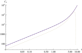
Figure 2: Temporal correlation as a function of time for $q=1.5$, when $R_{e}=10000$ (solid line), $1000$ (dashed line) and $100$ (dotted line).

Figure 3: Same as in Fig. 2, except for non-rotating flow.

III.1.2 Numerical solutions

Figure 1 shows that with the decrease of $q$, temporal correlation of velocity perturbation decreases as the fluctuation due to the presence of Coriolis force increases. At small values of $q$ (e.g. for $1,1.5$), however, the Coriolis fluctuation interacting with noise appears to be dominating in a way that the correlation reveals an oscillatory amplitude (this is more clear from Fig. 2). Hence in a few rotation time the correlation exceeds that of large $q$, when it increases steadily in absence of dominant Coriolis effect at large $q$. However, in either of the regimes, temporal correlation of perturbation appears large enough in a few rotation time, which reveals nonlinearity in the system, presumably leading to instability. The correlation appears to be increasing steadily for the nonrotating case, in absence of Coriolis fluctuation, similar to that for $q\rightarrow 2$. Thus the interesting outcome here is the following. The Coriolis fluctuations along with a steady effect of noise lead to a larger $C_{u}(\tau)$ for a smaller $q$ than that of a larger $q$ in a few rotation time, as is also indicated by equation (18). Note that an important physical quantity in this context is the rotation time of the flow. In a few rotation time, noise and the Coriolis fluctuation together bring in a large $C_{u}(\tau)$ and hence perturbation energy (prone to a smaller $q$, such as $1.5$), which presumably could lead to a transition to turbulence. Therefore, the presence of noise makes the Coriolis effect active to generate instability, which were otherwise acting as the agents hindering the perturbation effects (see, e.g. man ; amn ), leading to a faster rate of perturbation energy growth into the system.

Figure 2 shows that for $q<2$, the correlation tends to become independent of $R_{e}$. This is because with decreasing $q$, the epicyclic frequency ($\kappa=\Omega\sqrt{2(2-q)}$) becomes larger bringing lots of fluctuation in the flow, which makes the flow limited by the dynamics itself but not by the viscosity. In absence of noise, perturbation energy growth (and hence $C_{u}(\tau)$) is very small, as shown previously man , for $q<2$, particularly in three dimensions. Note, however, that at a small/moderate $R_{e}$, epicyclic fluctuations work with noise in such a way that $C_{u}(\tau)$ at small $\tau$ appears smaller than that of larger $R_{e}$ (see $R_{e}=100$ case in Fig. 2) due to the harmonic nature of fluctuations. This effectively argues that the correlation saturates only with the increase of $R_{e}$ for $q<2$.

Figure 3 shows that $C_{u}(\tau)$ for a nonrotating flow at $R_{e}=100$ appears larger at large $\tau$ compared to that at larger values of $R_{e}$. This is due to the effect of noise, which would have been suppressed at larger $R_{e}$. This is also clearly understood from the analytical scaling laws given by equation (19). Note that, a very large $R_{e}$ along with a large $\tau$ diminishes fluctuations in the flow leading to a linear perturbation growth with $R_{e}$, as shown in equation (19c).

Comparing rotating and non-rotating cases, it can be further inferred that the noise suppresses the viscous effects in the rotating flow making it independent of $R_{e}$ in the regime of smaller $\tau$, as also shown by equation (18b). However, the optimum perturbation of a flow might reveal the correlation varying with $R_{e}$, and the above inferences are valid for a fixed perturbation, considered for all the present cases.

Note that in absence of noise, perturbation energy growth (and hence $C_{u}(\tau)$) in all the above rotating cases, essentially for $q<2$, is very small, as shown previously man , particularly in three dimensions. However, the effects of noise bring a steady growth in the perturbation top of the Coriolis fluctuations. A remarkable feature in the scaling nature of all these correlations, atleast for asymptotic $\tau$ (see, e.g., equations (18b) and (18c)), is their independence of $q$ (background angular velocity profile) — a trait identified in statistical physics literature as universality. All these flows, with identical overall perturbation energy growth exponents barabasi_stanley in asymptotic limits of $\tau$ (and also $R_{e}$), but generally with varying energy dissipation amplitudes, indicate a specific universality class for them.

III.2 Spatial correlation

Here also we assume $<\tilde{{\eta}_{1}}_{\vec{k},\omega}\,\tilde{{\eta}_{2}}_{\vec{k},\omega}>=0$ like temporal correlation and obtain spatial correlations of velocity, vorticity and gradient of velocity, given below as

$$<u(\vec{x},t)\,u(\vec{x}+\vec{r},t)>=S_{u}(r)=\int d^{3}k\,d\omega\,e^{i\vec{k}.\vec{r}}<\tilde{u}_{\vec{k},\omega}\,\tilde{u}_{-\vec{k},-\omega}>,$$

$$<\zeta(\vec{x},t)\,\zeta(\vec{x}+\vec{r},t)>=S_{\zeta}(r)=\int d^{3}k\,d\omega\,e^{i\vec{k}.\vec{r}}<\tilde{\zeta}_{\vec{k},\omega}\,\tilde{\zeta}_{-\vec{k},-\omega}>,$$

$${\hskip-36.98866pt<\frac{\partial u(\vec{x},t)}{\partial x}\,\frac{\partial u(\vec{x}+\vec{r},t)}{\partial x}>=S_{du}(r)=\int d^{3}k\,d\omega\,e^{i\vec{k}.\vec{r}}k_{x}^{2}<\tilde{u}_{\vec{k},\omega}\,\tilde{u}_{-\vec{k},-\omega}>},$$ (20)

where $\vec{r}$ be the position where the correlations to be measured.

Now using equations (8), (11), (12) and (20), the velocity correlation perturbation $S_{u}(r)$ is explicitly given by

$$S_{u}(r)=2\pi\int_{k_{0}}^{k_{m}}~{}dk~{}k^{2}~{}\int_{0}^{\pi}~{}d\theta~{}e^{ikr\cos\theta}~{}\int d\omega~{}[2D_{1}q^{4}R_{e}^{2}$$

$$(k^{4}+(R_{e}\omega+LR_{e}k_{y})^{2})+8D_{2}q^{2}R_{e}^{4}k_{z}^{2}]/[4(2-q)^{2}R_{e}^{4}k_{z}^{4}+$$

$$4R_{e}^{2}q^{2}(2-q)k^{2}k_{z}^{2}(k^{4}-(R_{e}\omega+LR_{e}k_{y})^{2})+k^{4}q^{4}(k^{4}+$$

$${(R_{e}\omega+LR_{e}k_{y})}^{2})^{2}]$$

$$=2\pi^{2}~{}\int_{k_{0}}^{k_{m}}~{}dk~{}k^{2}~{}J_{0}(kr)~{}\int d\omega~{}[2D_{1}q^{4}R_{e}^{2}(k^{4}+(R_{e}\omega+LR_{e}k_{y})^{2})$$

$$+8D_{2}q^{2}R_{e}^{4}k_{z}^{2}]/[4(2-q)^{2}R_{e}^{4}k_{z}^{4}+4R_{e}^{2}q^{2}(2-q)k^{2}k_{z}^{2}(k^{4}-(R_{e}$$

$$\omega+LR_{e}k_{y})^{2})+k^{4}q^{4}(k^{4}+(R_{e}\omega+LRk_{y})^{2})^{2}],$$ (21)

where $J_{0}(kr)$ is the zeroth-order Bessel function. Similarly, one can obtain $S_{\zeta}(r)$ and $S_{du}(r)$ explicitly, when the poles in equation (21) are exactly the same as that given by equation (LABEL:poles). Here also we stick to the simplifying assumption $k_{x}=k_{y}=k_{z}=k/\sqrt{3}$.

Now following the same procedure as applied for the correlation of temporal velocity perturbation, we obtain the correlation of spatial velocity perturbation $S_{u}(r)$ given by

$$S_{u}(r)=\int_{k_{0}}^{k_{m}}~{}dk~{}k^{2}~{}J_{0}(kr)~{}{\rm RES}_{S_{u}}(q,R_{e},r),$$ (22)

where ${\rm RES}_{S_{u}}(q,R_{e},r)$ is the magnitude of the part arising from frequency integration.

III.2.1 Asymptotic scaling laws

At large $r$ and $R_{e}$ (which is a natural/astrophysical scenario), the flows with all $q$ reveal identical scaling of correlation with $r$ given by

$${S_{u}}_{(R_{e}\,{\rm and}\,r\rightarrow\infty)}\rightarrow\frac{\pi^{3/2}q}{r^{1/2}}\,(2-q)^{-3/2}\,\int_{k_{0}}^{k_{m}}dk\,\exp(-kr)\,\frac{2\sqrt{3}(k^{2}-1)+q\sqrt{3}}{k^{5/2}}$$ (23)

which is independent of $R_{e}$. Note that at a finite $r$, $\exp(-kr)/\sqrt{r}\rightarrow J_{0}(kr)$. Hence, the flow is limited by dynamics. This reveals identical roughness exponents barabasi_stanley for all flows, indicating a single universality class, as was already predicted from the temporal correlations. Equation (23) also reveals a steadily damped instability. It further recovers the fact that the flow exhibits unbounded correlation as $q\rightarrow 2$, and hence unbounded growth of perturbation. At small $r$

$${S_{u}}_{(R_{e}\rightarrow\infty,\,\,r\rightarrow 0)}\rightarrow-q\,(2-q)^{-3/2}\int_{k_{0}}^{k_{m}}dk\,\frac{(2-q-2k^{2})\log\left(\frac{kr}{2}\right)}{k^{2}},$$

(24)

which is again determined by rotational parameter $q$ only, when $\log(kr/2)$ becomes negative at a small $r$. Hence, except $q=2$ (or $q$ very very close to $2$) and/or $r=0$ (or $r$ very very close to $0$), the correlation is finite.

Figure 4: Spatial correlation as a function of radial coordinate for $R_{e}=10000$, when $q=1$ (solid line), $1.5$ (dashed line), $1.9$ (dotted line), $1.9999$ (dotdashed line) and flow is non-rotating (thick line).

Figure 5: Spatial correlation as a function of radial coordinate for $q=1.5$, when $R_{e}=10000$ (solid line), $1000$ (dashed line) and $100$ (dotted line).

Figure 6: Same as in Fig. 5, except for non-rotating flow.

For completeness, we also describe scaling laws for nonrotating flows. At large $r$ and $R_{e}$

$${S_{u}}_{(R_{e}\,{\rm and}\,r\rightarrow\infty)}^{\rm nonrot}\rightarrow\frac{R_{e}\,\pi^{3/2}\sqrt{2}}{r^{1/2}}\int_{k_{0}}^{k_{m}}dk\,\frac{\exp(-kr)}{k^{9/2}},$$ (25)

which scales with $R_{e}$, unlike the rotating flows. Hence the flow is not limited by dynamics at any $r$. However, at $r\rightarrow 0$ the scaling behavior changes and is given by

$${S_{u}}_{(R_{e}\rightarrow\infty,\,\,r\rightarrow 0)}^{\rm nonrot}\rightarrow-2R_{e}\pi\int_{k_{m}}^{k_{0}}dk\,\frac{\log\left(\frac{kr}{2}\right)}{k^{4}},$$ (26)

which still scales linearly with $R_{e}$.

III.2.2 Numerical solutions

Figures 4-5 show that the spatial correlations of perturbation decrease with the decrease of $q$ from $2$, when the epicyclic fluctuations arise into the flow. Moreover, the correlations for all $R_{e}$ tend to merge at large $r$, at a given $q$ particularly, becoming independent of $R_{e}$, as is also shown by the asymptotic result given by equation (23). However, at small $r$ and finite $R_{e}$, they depend on viscosity. This is due to the effect of noise, as is the case for temporal correlations.

On the other hand, for non-rotating flows, the correlations are not limited by the dynamics of the flow, as shown by Fig. 6, rather are controlled by viscosity. This is also understood from equations (25) and (26). Hence, the rotational effects constraint the correlation noticeably.

It is generally seen that the correlations decrease with increasing $r$ and decreasing $q$. Note their exponential decaying nature in equations (23) and (25) compared to the logarithmic variance in equations (24) and (26). However, their value appears significant enough to reveal a steadily damped instability in the flow. The possibilities of steadily damped oscillatory instabilities in constrained Orr-Sommerfeld flows were already predicted in two dimensions akhavan91 as well in the recirculating cavities between the jets produced behind a high solidity grid consisting of a perforated plate villermaux91 .

All the above correlations are computed for white noise. Figures 7 and 8 show the variations of spatial correlations of velocity perturbation for color noise respectively without and with vertex corrections in $D_{i}(k)$. Interestingly, while the magnitude of correlations decreases with respect to that for white noise (particularly for $D_{1}=D_{2}\sim 1/k^{3}$), with the increase of $q$ they appear large enough to govern instability. As an example, for noise with vertex correction, the Keplerian flow still reveals large enough correlation even at small radial coordinates.

All the above large values of perturbation energy growth are indicative of pure hydrodynamic instability and plausible turbulent transport, which is one of the outcomes under this theory.

Figure 7: Same as in Fig. 4, except for $D_{1}=D_{2}\sim 1/k^{3}$.

Figure 8: Same as in Fig. 4, except for $D_{1}=D_{2}\sim 1/k$.

III.3 Spectrum

In order to compute the spectrum of flow, let us first integrate $\omega$-part of equation (21) and obtain

$$\int E_{u}(k)~{}dk=\int d^{3}k~{}{\rm RES}_{S_{u}}(q,R_{e},k,D_{1},D_{2}).$$ (27)

Similarly, one can obtain $\int E_{\zeta}(k)dk$ and $\int E_{du}(k)dk$ from $S_{\zeta}$ and $S_{du}$ respectively. They would scale in a same way as of $\int E_{u}(k)dk$. Hence, the energy spectrum can generally be given by

$$E_{u}(k)=C~{}k^{2}~{}{\rm RES}_{S_{u}}(q,R_{e},k,D_{1},D_{2}),$$ (28)

when $C$ is a constant. Figures 9 and 10 show that the energy spectra for all the rotating flows with $q<2$ have same spectral indices at large and small $k$. Moreover, the energy appears identical for all $q$ at large $k$, which is due to the fact that a small length scale appears identical for all rotational profiles. At large scale, the spectral index is same as that of noise correlation, which implies that the flow is controlled by noise in that regime. However, interestingly, there is no change of slop in the nonrotating case, and the corresponding power-law index appears same as that of the large $k$ rotating ones. This may be understood as the Coriolis force in the rotating flows distorts the system which results in affecting the large scale (and hence small $k$) behavior of the flow. Hence, the behavior of non-rotating flow appears same throughout without being affected by the rotational effects. Note also that the color noise increases the power-law indices throughout compared to that for white noise.

Figure 9: Energy spectra for the velocity perturbation, when $q=1$ (dashed line), $1.5$ (dotted line) and $1.9$ (dotdashed line) and flow is nonrotating (longdashed). The solid and thick-solid lines respectively indicate the nature of slop of the curves at small and large $k$ for rotating flows. $D_{1}=D_{2}=1$, $R_{e}=10000$.

Figure 10: Same as in Fig. 9, except for $D_{1}=D_{2}\sim 1/k^{3}$.

IV Summary and conclusion

We have attempted to address the origin of instability and then turbulence in rotating shear flows (more precisely a small section of it, which is a plane shear flow with the Coriolis force). Our particular emphasis is the flows having angular velocity decreases but specific angular momentum increases with the radial coordinate, which are Rayleigh stable. The flows with such a kind of velocity profiles are often seen in astrophysics. As the molecular viscosity in astrophysical accretion disks is negligible, any transport of matter therein would arise through turbulence. However, the Rayleigh stable flows, particularly in absence of magnetic coupling, could not reveal any unstable mode which could serve as a seed of turbulence. Therefore, essentially we have addressed the plausible origin of pure hydrodynamic turbulence in rotating shear flows of the kind mentioned above. This is particularly meaningful for charge natural flows like accretion disks around quiescent cataclysmic variables, in protoplanetary and star-forming disks, and the outer region of disks in active galactic nuclei etc. where flows are cold and of low ionization and effectively neutral in charge. Note that whether a flow is magnetically arrested or not, the magnetic instability is there or not, hydrodynamic effects always exist. Hence, the relative strengths of hydrodynamics and hydromagnetics in the time scale of interest determines the actual source of instability.

We have shown, based on the theory of statistical physics, that stochastically forced linearized rotating shear flows in a narrow gap limit reveal a large correlation energy growth of perturbation in presence of noise. While the correlations are directly proportional to the Reynolds number for nonrotating flows, they are independent or weakly dependent of Reynolds number for rotating flows. Hence the later flows are mostly controlled by the dynamics and noise. While correlations of perturbation decrease as the flow deviates from the type of constant specific angular momentum to of the Keplerian and then to of constant circular velocity, still they appear large enough to trigger nonlinear effects and instability.

While earlier the origin of hydrodynamic instability in rotating shear flows of said kind was addressed based on “bypass method” in two dimensions man ; amn , it was shown that bm06 extra physics, e.g. elliptical vortex effects, has to be invoked for such instabilities to occur in three dimensions. However, later theories showing instabilities are effectively based on nonlinear theory. Therefore, the present work addresses the large three-dimensional hydrodynamic energy growth of linear perturbation for the first time, in such rotating flows, to best of our knowledge, which presumably leads to instability and subsequent turbulence in such flows. Only requirement here is to have the presence of stochastic noise in the system, which is quite obvious in natural flows like astrophysical accretion disks. Indeed, to best of our knowledge, no one so far has addressed the effects of stochastic noise in such rotating flows.

Interestingly, the flows with velocity profile $\Omega\sim r^{-q}$, with $q<2$, exhibiting identical overall growth exponents (but may not be identical energy dissipation amplitudes), indicate a specific universality class. At large $r$, they also reveal identical roughness exponents. Thus the properties of temporal and spatial correlations together indicate the Rayleigh stable rotating shear flows to follow a single universality class.

Let us end by clarifying suitability of astrophysical application of our results which is based on incompressible assumption. If the wavelength of the velocity perturbations is much shorter than the sound horizon for the time of interest (e.g. infall time of matter), then the density perturbations (i.e. sound waves) reach equilibrium early on, exhibiting effectively uniform density during the timescale of interest. For a geometrically thin astrophysical accretion disk around a gravitating mass, the vertical half-thickness of the disk ($h$) is comparable to the sound horizon corresponding to one disk rotation time prin such that $h\sim c_{s}/\Omega$. Therefore, as described in previous work chage ; yeko ; amn ; jg05 ; umregmen ; rajesh , for processes taking longer than one rotation time, wavelengths shorter than the disk thickness can be approximately treated as incompressible. A detailed astrophysical application of the present work has been reported elsewhere mukhch .

Appendix: Magnetic version of the set of Orr-Sommerfeld and Squire equations

Let us now establish the linearized Navier-Stokes equation in presence of background plane shear $(0,-x,0)$ without neglecting magnetic coupling with a background magnetic field $(0,B_{1},1)$, when $B_{1}$ being a constant, in presence of angular velocity $\Omega\sim r^{-q}$ in a small section of the incompressible flow. Hence, the underlying equations are nothing but the linearized set of hydromagnetic equations including the equations of induction in local Cartesian coordinates (see, e.g., man ; bmraha for detailed description of the choice of coordinate in a small section) given by

$$\left(\frac{\partial}{\partial t}-x\frac{\partial}{\partial y}\right)u-\frac{2v}{q}+\frac{\partial p_{\rm tot}}{\partial x}-\frac{1}{4\pi}\left(B_{1}\frac{\partial B_{x}}{\partial y}+\frac{\partial B_{x}}{\partial z}\right)=\frac{1}{R_{e}}\nabla^{2}u,$$ (29)

$$\left(\frac{\partial}{\partial t}-x\frac{\partial}{\partial y}\right)v+\left(\frac{2}{q}-1\right)u+\frac{\partial p_{\rm tot}}{\partial y}-\frac{1}{4\pi}\left(B_{1}\frac{\partial B_{y}}{\partial y}+\frac{\partial B_{y}}{\partial z}\right)=\frac{1}{R_{e}}\nabla^{2}v,$$ (30)

$$\left(\frac{\partial}{\partial t}-x\frac{\partial}{\partial y}\right)w+\frac{\partial p_{\rm tot}}{\partial z}-\frac{1}{4\pi}\left(B_{1}\frac{\partial B_{z}}{\partial y}+\frac{\partial B_{z}}{\partial z}\right)=\frac{1}{R_{e}}\nabla^{2}w,$$ (31)

$$\frac{\partial B_{x}}{\partial t}=\frac{\partial u}{\partial z}+B_{1}\frac{\partial u}{\partial y}+x\frac{\partial B_{x}}{\partial y}+\frac{1}{R_{m}}\nabla^{2}B_{x},$$ (32)

$$\frac{\partial B_{y}}{\partial t}=\frac{\partial v}{\partial z}+B_{1}\frac{\partial v}{\partial y}-x\frac{\partial B_{x}}{\partial x}-x\frac{\partial B_{z}}{\partial z}-B_{x}+\frac{1}{R_{m}}\nabla^{2}B_{y},$$ (33)

$$\frac{\partial B_{z}}{\partial t}=\frac{\partial w}{\partial z}+B_{1}\frac{\partial w}{\partial y}+x\frac{\partial B_{z}}{\partial y}+\frac{1}{R_{m}}\nabla^{2}B_{z},$$ (34)

when the vectors for velocity and magnetic field perturbations are $(u,v,w)$ and $(B_{x},B_{y},B_{z})$ respectively, $R_{e}$ and $R_{m}$ are the hydrodynamic and magnetic Reynolds numbers respectively, $p_{\rm tot}$ is the total pressure perturbation (including that due to the magnetic field). Above equations are supplemented by the conditions for incompressibility and no magnetic charge, given by

$$\frac{\partial u}{\partial x}+\frac{\partial v}{\partial y}+\frac{\partial w}{\partial z}=0,$$ (35)

$$\frac{\partial B_{x}}{\partial x}+\frac{\partial B_{y}}{\partial y}+\frac{\partial B_{z}}{\partial z}=0.$$ (36)

Now by taking partial derivatives with respect to $x,y,z$ respectively to both the sides of equations (29), (30), (31) and adding them up we obtain

$$\nabla^{2}p_{\rm tot}=\frac{2}{q}\left(\frac{\partial v}{\partial x}-\frac{\partial u}{\partial y}\right)+2\frac{\partial u}{\partial y}.$$ (37)

Now taking $\nabla^{2}$ to equation (29), using equation (37) and defining $x$-component of vorticity $\zeta={\partial w}/{\partial y}-{\partial v}/{\partial z}$, we obtain

$$\left(\frac{\partial}{\partial t}-x\frac{\partial}{\partial y}\right)\nabla^{2}u+\frac{2}{q}\frac{\partial\zeta}{\partial z}-\frac{1}{4\pi}\left(B_{1}\frac{\partial}{\partial y}+\frac{\partial}{\partial z}\right)\nabla^{2}B_{x}=\frac{1}{R_{e}}\nabla^{4}u.$$ (38)

Also by taking partial derivatives with respect to $x$ and $y$ respectively to both the sides of equations (30), (29) respectively, subtracting one from other and defining $\zeta_{B}={\partial B_{z}}/{\partial y}-{\partial B_{y}}/{\partial z}$, we obtain

$$\left(\frac{\partial}{\partial t}-x\frac{\partial}{\partial y}\right)\zeta+\left(1-\frac{2}{q}\right)\frac{\partial u}{\partial z}-\frac{1}{4\pi}\left(B_{1}\frac{\partial}{\partial y}+\frac{\partial}{\partial z}\right)\zeta_{B}=\frac{1}{R_{e}}\nabla^{2}\zeta.$$ (39)

Furthermore, by taking partial derivatives with respect to $y$ and $z$ respectively to both the sides of equations (34) and (33) and subtracting one from other, we obtain

$$\left(\frac{\partial}{\partial t}-x\frac{\partial}{\partial y}\right)\zeta_{B}=\frac{\partial\zeta}{\partial z}+B_{1}\frac{\partial\zeta}{\partial y}+\frac{\partial B_{x}}{\partial z}+\frac{1}{R_{m}}\nabla^{2}\zeta_{B}.$$ (40)

The equations (38), (39), (32) and (40) describe the set of magnetized version of the Orr-Sommerfeld and Squire equations in presence of the Coriolis force, for the background magnetic field described above and linear shear. To best of our knowledge, this set of equations has not been reported in the existing literature so far.

References

- (1) Chagelishvili, G. D., Zahn, J.-P., Tevzadze, A. G., Lominadze, J. G., A&A 402, 401 (2003).
- (2) Tevzadze, A. G., Chagelishvili, G. D., Zahn, J.-P., Chanishvili, R. G.& Lominadze, J. G., A&A 407, 779 (2003).
- (3) Yecko, P. A., A&A 425, 385 (2004).
- (4) Mukhopadhyay, B., Afshordi, N. & Narayan, R., ApJ 629, 383 (2005).
- (5) Afshordi, N., Mukhopadhyay, B. & Narayan, R., ApJ 629, 373 (2005).
- (6) Butler, K. M., & Farrell, B. F., Phys. Flud. 4, 1637 (1992).
- (7) Reddy, S. C., & Henningson, D. S., J. Flud. Mech. 252, 209 (1993).
- (8) Trefethen, L. N., Trefethen, A. E., Reddy, S. C., & Driscoll, T. A., Science 261, 578 (1993).
- (9) Farrell, B. F., Phys. Fluids 31(8), 2093 (1988).
- (10) Mukhopadhyay, B, Mathew, R., & Raha, S., NJPh 13, 023029 (2011).
- (11) Ji, H., Burin, M., Schartman, E., & Goodman, J., Nature 444, 343 (2006).
- (12) Paoletti, M. S., & Lathrop, D. P., Phys. Rev. Lett. 106, 024501 (2011).
- (13) Avila, M., Phys. Rev. Lett. 108, 124501 (2012).
- (14) Mukhopadhyay, B., & Saha, K., RAA 11, 163 (2011).
- (15) Mukhopadhyay, B., ApJ 653, 503 (2006).
- (16) Rajesh, S. R., MNRAS 414, 691 (2011).
- (17) Chandrasekhar, S., Hydrodynamics and Hydromagnetic Stability (Oxford University Press, 1961).
- (18) Batchelor, G. K., An Introduction to Fluid Mechanics (Cambridge University Press, 2000).
- (19) Forster, D., Nelson, D. R., & Stephen, M. J., Phys. Rev. A 16, 732 (1977).
- (20) De Dominicis, C., & Martin, P. C., Phys. Rev. A 19, 419 (1979).
- (21) Kolmogorov, A. N., Dokl. Akad. Nauk SSSR 30, 301 (1941).
- (22) Kolmogorov, A. N., J. Flud. Mech. 13, 82 (1962).
- (23) Bhattacharjee, J. K., Phys. Rev. Lett. 77, 1524 (1996).
- (24) Kardar, M., Parisi, G., & Zhang, Y.-C., Phys. Rev. Lett. 56, 889 (1986).
- (25) Chekhlov, A. & Yakhot, V., Physical Review E 51, 2739 (1995).
- (26) Chattopadhyay, A. K. & Bhattacharjee, J. K., Europhys. Lett. 42, 119 (1998).
- (27) Barabási, A.-L. & Stanley, H. E., Fractal concepts in surface growth (Cambridge University Press, 1995).
- (28) Medina, E., Hwa, T., Kardar, M., & Zhang, Y.-C., Phys. Rev. A 39, 3053 (1989).
- (29) Chattopadhyay, A. K., & Bhattacharjee, J. K., Phys. Rev. E 63, 016306 (2001).
- (30) Landau, L. D. & Lifshitz, E. M., Fluid Mechanics: Volume 6 (Course of Theoretical Physics) (Butterworth-Heinemann, 1987).
- (31) Jacobi, I., & Mckeon, B. J., J. Flud. Mech. 677, 179 (2011).
- (32) Meneveau, C., & Katz, J., Ann. Rev. Flud. Mech. 32, 1 (2000).
- (33) Misra, R., Harikrishnan, K. P., Mukhopadhyay, B., Ambika, G. & Kembhavi, A. K., ApJ 609, 313 (2004).
- (34) Karak, B. B., Dutta, J. & Mukhopadhyay, B., ApJ 708, 862 (2010); ApJ 715, 697 (2010).
- (35) Rajesh, S. R. & Mukhopadhyay, B., MNRAS 402, 961 (2010).
- (36) Mukhopadhyay, B. & Ghosh, S., MNRAS 342, 274 (2003).
- (37) Balbus, S. A., & Hawley, J. F., ApJ 376, 214 (1991).
- (38) Akhavan, R., Kamm, R. D. & Shapiro, A. H., J. Flud. Mech. 225, 423 (1991).
- (39) Villermaux, E., Gagne, Y., Hopfinger, E. J. & Sommeria, J., Euro. J. Mech. B Flud. 10, 427 (1991).
- (40) Pringle, J. E., ARA&A 19, 137 (1981).
- (41) Johnson, B. M., & Gammie, C. F., ApJ 635, 149 (2005).
- (42) Umurhan, O. M., Menou, K., & Regev, O., Phys. Rev. Lett. 98, 034501 (2007).
- (43) Mukhopadhyay, B., & Chattopadhyay, A. K., in the Proceedings of International Conference on Astrophysics and Cosmology, in Tribhuvan University, Kirtipur, Nepal, March 19-21, 2012.