The Optical Colors of Giant Elliptical Galaxies and their Metal-Rich Globular Clusters Indicate a Bottom-Heavy Initial Mass Function

Abstract

We report a systematic and statistically significant offset between the optical ($g\!-\!z$ or $B\!-\!I$) colors of seven massive elliptical galaxies and the mean colors of their associated massive metal-rich globular clusters (GCs) in the sense that the parent galaxies are redder by $\sim$ 0.12 – 0.20 mag at a given galactocentric distance. However, spectroscopic indices in the blue indicate that the luminosity-weighted ages and metallicities of such galaxies are equal to that of their averaged massive metal-rich GCs at a given galactocentric distance, to within small uncertainties. The observed color differences between the red GC systems and their parent galaxies cannot be explained by the presence of multiple stellar generations in massive metal-rich GCs, as the impact of the latter to the populations’ integrated $g\!-\!z$ or $B\!-\!I$ colors is found to be negligible. However, we show that this paradox can be explained if the stellar initial mass function (IMF) in these massive elliptical galaxies was significantly steeper at subsolar masses than canonical IMFs derived from star counts in the solar neighborhood, with the GC colors having become bluer due to dynamical evolution, causing a significant flattening of the stellar MF of the average surviving GC.

1. Introduction

The shape of the stellar initial mass function (IMF) is a fundamental property for studies of star and galaxy formation. It constitutes a crucial assumption when deriving physical parameters from observations. However, its origin remains relatively poorly understood. A particularly important question is whether or not the IMF is “universal” among different environments, since galactic mass-to-light (${\cal{M}}/L$) ratios are very sensitive to variations in the shape of the IMF at subsolar masses. Several observational studies find that the IMF in various environments within our Galaxy and the Magellanic Clouds seems remarkably uniform down to detection limits of $\sim 0.1-1\,M_{\odot}$ (Kroupa, 2001; Chabrier, 2003; Bastian et al., 2010, and references therein). However, recent studies indicate that the IMF may be different in more extreme environments: strong gravity-sensitive features in near-IR spectra of luminous elliptical galaxies by van Dokkum & Conroy (2010, 2011) favor a bottom-heavy IMF ($\alpha\simeq-3$ in $dN/d{\cal{M}}\propto{\cal{M}}^{\alpha}$). If confirmed, this result would have widespread implications on studies of stellar populations and galaxy evolution. For example, such a bottom-heavy IMF would increase the ${\cal{M}}/L$ ratio in the $K$ band by a factor $\sim$ 3 relative to a “standard” Kroupa (2001) IMF, and hence invalidate the widespread assumption that ${\cal{M}}/L$ ratios in the near-IR are highly independent of galaxy type or mass.

In this paper, we describe an effort to find independent evidence to confirm or deny the presence of a bottom-heavy IMF in nearby giant elliptical galaxies. We use observed optical colors and spectral line indices of metal-rich globular clusters (GCs) and their parent galaxies in conjunction with dynamical evolution modeling of GCs.

Infrared studies of star formation within molecular clouds have shown that stars form in clusters or unbound associations with initial masses ${\cal{M}}_{\rm cl,\,0}$ in the range $10^{2}-10^{8}$ $M_{\odot}$ (e.g., Lada & Lada, 2003; Portegies Zwart et al., 2010; Kruijssen, 2012, and references therein). While most star clusters with ${\cal{M}}_{\rm cl,\,0}\lesssim 10^{4}$ $M_{\odot}$ are thought to disperse into the field population of galaxies within a few Gyr, the surviving massive GCs constitute luminous compact sources that can be observed out to distances of several tens of megaparsecs. Furthermore, star clusters represent very good approximations of a “simple stellar population” (hereafter SSP), i.e., a coeval population of stars with a single metallicity, whereas the diffuse light of galaxies is typically composed of a mixture of different populations. Thus, star clusters represent invaluable probes of the star formation rate (SFR) and chemical enrichment occurring during the main star formation epochs within a galaxy’s assembly history.

Deep imaging studies with the Hubble Space Telescope (HST) revealed that giant elliptical galaxies typically contain rich GC systems with bimodal color distributions (e.g., Kundu & Whitmore, 2001; Peng et al., 2006). Follow-up spectroscopy showed that both “blue” and “red” GC subpopulations are nearly universally old, with ages $\gtrsim$ 8 Gyr (e.g., Cohen et al., 2003; Puzia et al., 2005; Brodie et al., 2012). This implies that the color bimodality is mainly due to differences in metallicity. The colors and spatial distributions of the blue GCs are usually consistent with those of metal-poor halo GCs in our Galaxy and M31, while red GCs have colors and spatial distributions that are similar to those of the “bulge” light of their host galaxies (e.g., Geisler et al., 1996; Rhode & Zepf, 2001; Bassino et al., 2006; Brodie & Strader, 2006; Peng et al., 2006; Goudfrooij et al., 2007). Thus, the red metal-rich GCs are commonly considered to be physically associated with the stellar body of giant elliptical galaxies. This represents an assumption for the remainder of this paper.

2. Galaxy Sample and GC Selection

Our main galaxy selection criterion is the presence of a very clear bimodal optical color distribution of its GCs as derived from high-quality, high spatial-resolution (i.e., HST) imaging that allows GC detection as close to the galaxy centers as possible. With this in mind, most galaxies in our sample were drawn from the ACS Virgo Cluster Survey (ACSVCS; Côté et al., 2004), a homogeneous survey of 100 early-type galaxies and their GCs in the Virgo galaxy cluster, using the F475W and F850LP filters (hereafter $g$ and $z$, respectively). Specifically, we use galaxy photometry from Ferrarese et al. (2006) supplemented by GC data from Jordán et al. (2009). Galaxies were selected based on the properties of GC color distributions as modeled by Peng et al. (2006) using the Kaye’s Mixture Model (KMM; McLachlan & Basford, 1988; Ashman et al., 1994), fitting two Gaussians to the data. Two criteria were used for selection: (i) the $p$-value of the KMM fit needs to be $\leq$ 0.01, and (ii) the color distribution of the GCs needs to clearly show two distinct peaks as judged by eye in Fig. 2 of Peng et al. (2006). Finally, we exclude NGC 4365 due to conflicting results on the presence of intermediate-age GCs among its red GCs in the literature. This selection yields the high-luminosity galaxies NGC 4472, NGC 4486, NGC 4649, NGC 4552, NGC 4621, and NGC 4473 (see Table 1).

In the context of the current study, it is important to include a comparison between metallicity measurements of red GCs from colors versus from spectral line indices (see Section 3 below). As adequate line index data for several red GCs is currently only available for one galaxy in the ACSVCS sample, we add NGC 1407 to our galaxy sample given that high-quality HST/ACS imaging (in filters F435W (hereafter $B$) and F814W ($I$)) as well as optical spectroscopy of both red GCs and the diffuse light are available (Forbes et al., 2006; Cenarro et al., 2007; Spolaor et al., 2008a, b).

The selection of red GCs in these galaxies was done by selecting GCs redder than the color for which the KMM probability of a GC being member of the blue versus the red peak is equal. In addition, we require GCs to be massive enough to render the effect of stochastic fluctuations of the number of red giant branch (RGB) and asymptotic giant branch (AGB) stars on the integrated colors smaller than the typical photometric error of $\sigma(g\!-\!z)$ = 0.04 mag. Using the methodology of Cerviño & Luridiana (2004) for an age of 12 Gyr and solar metallicity, this requirement translates in a minimum cluster mass ${\cal{M}}_{\rm cl}\simeq 2.5\times 10^{5}\>M_{\odot}$. For galaxies in the Virgo cluster, this mass limit is equivalent to selecting GCs with $z_{\rm AB}\leq 21.91$ mag under the assumptions of (i) ${\cal{M}}_{\rm cl}/L_{z}$ = 1.5 $M_{\odot}/L_{z,\odot}$ for $Z=Z_{\odot}$ (this value varies only slightly with metallicity; Jordán et al., 2007) and (ii) $m\!-\!M$ = 31.09 mag for the Virgo cluster (Jordán et al., 2009). The equivalent magnitude limit for the GCs in NGC 1407 is $I\leq 23.28$ mag, using ${\cal{M}}_{\rm cl}/L_{I}$ = 2.1 $M_{\odot}/L_{I,\odot}$ for $Z=Z_{\odot}$ (Maraston, 2005) and $m\!-\!M$ = 31.60 mag (Forbes et al., 2006).

3. Radial Color Gradients of Galaxies and their Red GC Systems

In this section we compare the colors of the red GCs (selected as mentioned above) with those of the diffuse light of their parent galaxies as a function of projected galactocentric radius (hereafter $R_{\rm gal}$). All observed colors for the ACSVCS galaxies were dereddened using the Galactic foreground reddening values listed in Jordán et al. (2009). The colors of GCs in NGC 1407 from Forbes et al. (2006) were already corrected for Galactic foreground reddening. For each galaxy we calculate a mean color of the red GC population along with its radial gradient by means of a weighted linear least-squares fit between the GC’s colors col (i.e., $g\!-\!z$ or $B\!-\!I$) and the logarithm of $R_{\rm gal}$ in arcsec:

$$\overline{\mbox{\it col}}\;(R_{\rm gal})={\it col}_{0}+G_{\it col}\>\log(R_{\rm gal})$$ (1)

where col₀ is the $g\!-\!z$ or $B\!-\!I$ color at log ($R_{\rm gal}$) = 0 and $G_{\it col}$ is the color gradient per dex in radius, $\Delta$(col)/$\Delta\log(R_{\rm gal})$. For each GC, uncertainties associated with its measured color and its membership of the red population are taken into account in the fit by adding the following two parameters in quadrature: (i) the photometric error of the GC’s color, and (ii) the inverse probability of the GC being a member of the red population ($p_{\rm red}$), as calculated by the KMM algorithm mentioned above, expressed in magnitudes (i.e., log($1/p_{\rm red}$) / log(2.5)). Radial color profiles for the diffuse light of the parent galaxies were determined using the same functional form as Eq. (1). For NGC 1407, $B\!-\!I$ data of the diffuse light were taken from the surface photometry of Spolaor et al. (2008a), which was derived from the same HST/ACS data as the GC photometry of Forbes et al. (2006). ACSVCS galaxy color gradients are taken from Liu et al. (2011), who used the surface photometry of Ferrarese et al. (2006). Observed ACSVCS galaxy colors at $R_{\rm gal}=1$ arcsec were taken from Ferrarese et al. (2006) and listed in Table 1. Panels (a) – (c) and (e) – (g) of Figure 1 show $g\!-\!z$ versus $R_{\rm gal}$ for the 6 ACSVCS galaxies and their massive red GCs. Panel (a) of Figure 2 shows the equivalent for NGC 1407 and its red GCs. Note that while the radial gradients of the galaxies’ colors are similar to those of the “average” colors of their red GC systems, there is a systematic offset between the two sets of radial color profiles in the sense that the average color of red GCs is $\simeq$ 0.12 – 0.20 mag bluer in $g\!-\!z$ or $B\!-\!I$ than that of their parent galaxies. This color difference was already noted by Peng et al. (2006), but they did not pursue an investigation of its possible cause(s). The significance of this color difference is 7 $\sigma$ to 22 $\sigma$ depending on the galaxy, where $\sigma$ is the mean error of the fit of eq. (1) to the colors of red GCs in the sample galaxies (see Table 1).

Table 1Colors of sample galaxies and their massive red GCs.

NGC	$M_{V^{0}_{T}}$	$(g\!-\!z)_{0,\,\rm gal}$	$(g\!-\!z)_{0}$	$G_{g\!-\!z}$	rms
(1)	(2)	(3)	(4)	(5)	(6)
4472	$-$22.90	1.586 $\pm$ 0.005	1.425	$-$0.021	0.010
4486	$-$22.66	1.598 $\pm$ 0.005	1.413	$+$0.000	0.007
4649	$-$22.41	1.592 $\pm$ 0.005	1.449	$-$0.022	0.010
4552	$-$21.36	1.558 $\pm$ 0.005	1.372	$+$0.000	0.014
4621	$-$21.18	1.596 $\pm$ 0.005	1.365	$-$0.023	0.013
4473	$-$20.70	1.563 $\pm$ 0.005	1.358	$-$0.005	0.017
NGC	$M_{V^{0}_{T}}$	$(B\!-\!I)_{0,\,\rm gal}$	$(B\!-\!I)_{0}$	$G_{B\!-\!I}$	rms
1407	$-$21.86	2.313 $\pm$ 0.005	2.103	$-$0.004	0.007

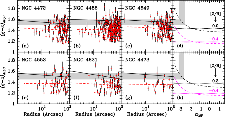
Figure 1.— Radial color gradients of giant elliptical galaxies from the ACSVCS survey and their systems of massive red GCs. Panels (a) – (c) and (e) – (g) show dereddened $(g\!-\!z)_{\rm AB}$ versus projected galactocentric radius for the ACSVCS galaxies mentioned at the top left of the panel in question. Black solid lines represent linear least-square fits to the galaxy colors, red circles with black error bars represent individual red GCs, and the red dashed lines depict linear least-square fits to the red GC systems as a whole. The dashed lines in panel (d) plot integrated $(g\!-\!z)_{\rm AB}$ versus mass function (MF) slope $\alpha_{\it MF}$ for Marigo et al. (2008) isochrones for an age of 12 Gyr and the two [$Z$/H] values shown in the legend. The dotted lines in panel (d) indicate the colors for a Kroupa (2001) MF. Panel (h) is similar to panel (d), but now the upper (black) lines are drawn for [$Z$/H] = $-$0.2. The grey shaded region crossing panels (a) through (d) and (e) through (h) illustrate the range of MF slopes reproducing the galaxy colors for the upper isochrone lines drawn in panels (d) and (h), respectively.

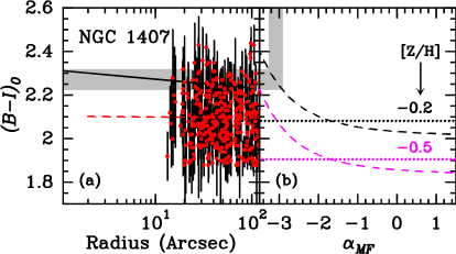
Figure 2.— Similar to Figure 1, but now for NGC 1407 and its red GCs. Panel (a) shows $(B\!-\!I)_{0}$ versus projected galactocentric radius. The dashed lines in panel (b) plot integrated $(B\!-\!I)_{0}$ versus MF slope $\alpha_{\it MF}$ for Marigo et al. (2008) isochrones for an age of 12 Gyr and the two [$Z$/H] values shown in the legend. Symbols, lines, and shading as in Figure 1.

Under the assumption that surviving GCs represent the high-mass end of the star formation process that also populated the field (Elmegreen & Efremov, 1997), this color difference is difficult to understand in terms of a metallicity difference. While we deem it likely that the spread of colors exhibited by the red GC systems in Figure 1 is due (at least in part) to a range of GC metallicities (and/or ages), one would expect that the same range of metallicities (and/or ages) be present among the field stars and hence that the average colors would be similar.

This argument is corroborated by spectroscopic Lick index data for red GCs and the diffuse light in the two giant elliptical galaxies in our sample (or in the literature at large) for which we found such data available in the literature for both a significant number of red GCs and the diffuse light within a range in $R_{\rm gal}$ sampled by both components. As to the GC spectra, Cohen et al. (2003) obtained Keck/LRIS spectra of 47 GCs in NGC 4472, while Cenarro et al. (2007) used Keck/LRIS to obtain spectra for 20 GCs in NGC 1407. In both studies, the resulting GCs were split approximately evenly between blue and red GCs. To evaluate spectroscopic ages and metallicities, we use the indices H$\beta$ and [MgFe]${}^{\prime}=\left(\mbox{Mg}\,b\times(0.72\,\mbox{Fe}_{5270}+0.28\,\mbox{Fe}_{5335})\right)^{1/2}$, respectively, and compare them to predictions of the SSP models of Thomas et al. (2003). The [MgFe]^′ metallicity index was chosen because Thomas et al. (2003) found it to be independent of variations in [$\alpha$/Fe] ratio. This is relevant since giant elliptical galaxies and their metal-rich GCs are known to exhibit supersolar $\alpha$/Fe ratios (e.g., Trager et al., 2000; Puzia et al., 2006). Figure 3 shows H$\beta$ versus [MgFe]^′ for the GCs in NGC 4472 from Cohen et al. (2003), subdivided into blue and red GCs. As the uncertainties are significant for the individual GCs, we also indicate weighted average indices for the blue and red GCs (see large blue and red symbols in Figure 3). Note that [$Z$/H] $\simeq+0.30$ for the average red GC in Figure 3, which corresponds to [$Z$/H] = $-0.07$ on the Zinn & West (1984) scale (Cohen et al., 2003). For comparison, we overplot H$\beta$ and [MgFe]^′ for the diffuse light of NGC 4472 (Davies et al., 1993; Fisher et al., 1995) at $R_{\rm gal}$ = 50^′′. Note that the median $R_{\rm gal}$ of the red GCs targeted by Cohen et al. (2003) is 59$\farcs$1. Similarly, Figure 4 shows H$\beta$ versus [MgFe]^′ for the blue and red GCs in NGC 1407 from Cenarro et al. (2007) and the diffuse light of NGC 1407 at $R_{\rm gal}$ = 50^′′ from Spolaor et al. (2008b). For comparison, the median $R_{\rm gal}$ of the red GCs targeted by Cenarro et al. (2007) is 50$\farcs$3. We conclude that the average red GC and the diffuse light have equal values of H$\beta$ and [MgFe]^′ to within 1$\sigma$ for both NGC 1407 and NGC 4472, the two galaxies for which we could find spectroscopic ages and metallicities for both red GCs and the diffuse light, at comparable galactocentric distances, in the literature. This indicates that the mean ages and metallicities of the red GCs and the underlying diffuse light of giant elliptical galaxies are indeed the same within the uncertainties.

We thus arrive at a situation where the mean spectroscopic ages and metallicities of the diffuse light of giant elliptical galaxies and their red GCs seem consistent with one another while the $g\!-\!z$ or $B\!-\!I$ colors of the diffuse light of the galaxies are systematically redder than those of their average red GC. We evaluate three possible solutions to this paradox below.

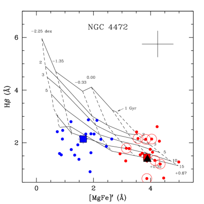
Figure 3.— H$\beta$ versus [MgFe]^′ for GCs in NGC 4472 from the data of Cohen et al. (2003). Small blue and red circles indicate GCs designated by Geisler et al. (1996) as “blue” and “red”, respectively. Large filled blue and red squares represent weighted average values of H$\beta$ and [MgFe]^′ of the blue and red GCs, respectively. Large open red circles indicate red GCs with HST/ACS photometry (see Figure 5a and Sect. 4.1). Error bars at the top right indicate typical uncertainties for individual GCs. SSP models of Thomas et al. (2003) are overplotted for [$\alpha$/Fe] = +0.3. Dashed lines indicate [$Z$/H] values of $-$2.25, $-$1.35, $-$0.33, 0.00, 0.35, and 0.67 dex. Solid lines indicate ages of 1, 2, 3, 5, 10, and 15 Gyr. For comparison, the black triangle represents H$\beta$ and [MgFe]^′ for the diffuse light of NGC 4472 at $R_{\rm gal}=50^{\prime\prime}$. See Sect. 3.

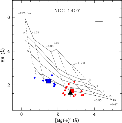
Figure 4.— Similar to Figure 3, but now for GCs in NGC 1407 from the data of Cenarro et al. (2007) and for the diffuse light of NGC 1407 at $R_{\rm gal}=50^{\prime\prime}$ from the data of Spolaor et al. (2008b). Large open red circles are not shown in this case since all GCs shown have HST/ACS photometry (cf. Figure 5b).

4. Possible Causes of the Color Offset Between Red GC Systems and Their Parent Galaxies

4.1. A Mismatch between Photometric and Spectroscopic Samples?

As a first possible solution to the paradox described in the previous Section, we consider the hypothesis that the red GCs in NGC 4472 and NGC 1407 whose spectroscopic Lick index data were shown in Figures 3 and 4, respectively, happen to be redder and more metal-rich on average than the respective full photometric samples of red GCs. This hypothesis is rejected by the data, as illustrated in Figure 5 in which open circles highlight the red GCs that have counterparts in Figures 3 and 4. Dotted black lines indicate the mean $g\!-\!z$ or $B\!-\!I$ colors of the GCs with Lick index data, which are consistent with the mean colors of the full red GC systems to within 1 $\sigma$. Recalling that the significance of the observed color differences between the metal-rich GC systems and their host galaxies is in the range 7 – 22 $\sigma$, we conclude that the red GCs with Lick index data are not misrepresenting the full systems of red GCs in terms of their $g\!-\!z$ or $B\!-\!I$ colors.

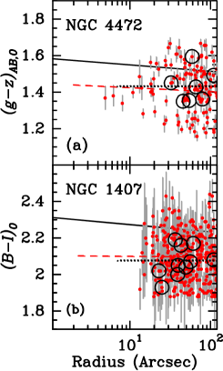
Figure 5.— Panels (a) and (b) are near-copies of Figures 1a and 2a, respectively, except that error bars are now shown in grey. Large open circles in panels (a) and (b) identify the red GCs in the HST data for which Lick index data were shown in Figures 3 and 4, respectively. The black dotted lines indicate the mean colors of the two sets of red GCs shown with large open circles. Note that the black dotted lines almost coincide with the red dashed lines, which depict linear fits to Eq. 1 for the full red GC systems.

4.2. An Effect of the Presence of Multiple Stellar Populations in Massive GCs?

Several detailed photometric and spectroscopic investigations over the last decade have established that massive Galactic GCs typically host multiple, approximately coeval, stellar populations (see the recent review by Gratton et al., 2012, and references therein). The recognition of this fact came mainly with the common presence of anticorrelations between [Na/Fe] and [O/Fe] among individual stars (often dubbed “Na-O anticorrelations”; see, e.g., Carretta et al., 2010), which are seen within virtually all Galactic GCs studied using multi-object spectroscopy with 8-m-class telescopes to date. The leading theory on the cause of these abundance variations is the presence of a second generation of stars formed out of enriched material lost (with low outflow velocity) by “polluters” (massive stars and/or intermediate-mass AGB stars) of the first generation. High-temperature proton-capture nucleosynthesis in the atmospheres of the “polluters” increased the abundances of He, N, and Na relative to Fe (e.g., Renzini, 2008).

Note that this theory only predicts observable star-to-star abundance variations among light elements (up to ¹³Al), which is consistent with what is seen among almost all Galactic GCs. Variations in heavy (e.g., Fe-peak) element abundances have only been found within two very massive metal-poor GCs: $\omega$ Cen (e.g. Lee et al., 2005; Johnson & Pilachowski, 2010) and M 22 (Marino et al., 2009). It is thought that such GCs represent surviving nuclei of accreted dwarf galaxies whose escape velocities were high enough to retain Fe-peak elements from SN explosions (e.g., Lee et al., 2007; Georgiev et al., 2009). However, we deem this accretion scenario rather unlikely for the formation history of red GCs given their high metallicities. We therefore restrict the following discussion to GCs without a spread in iron abundance.

The effect of light-element abundance variations within GCs to photometry seems to be more subtle than that to spectroscopic line indices. While photometric splitting of RGB, main sequence (MS), and/or subgiant branch (SGB) sequences have been observed in color-magnitude diagrams (CMDs) of several Galactic GCs, such splits only show up in CMDs that involve filters shortward of $\sim$ 4000 Å, while they disappear when using visual passbands such as $B$, $V$, and/or $I$ (see, e.g., Marino et al., 2008; Kravtsov et al., 2011; Milone et al., 2012).

To evaluate the effect of the presence of multiple stellar populations in massive GCs to their colors, we determine colors of various stellar types from synthetic spectra with chemical compositions typical of first– and second-generation stars found in massive GCs, and we use the resulting stellar spectra to calculate integrated colors of the full stellar population. This procedure is described in detail in Appendix A. As shown there, the expected impact of the presence of two stellar generations to the integrated $B\!-\!I$ and $g\!-\!z$ colors of metal-rich GCs is offsets of $-$0.021 and $-$0.027 mag, respectively, relative to a true SSP. As this is only a small fraction of the observed color offsets between red GC systems and the diffuse light of giant elliptical galaxies, it seems that an additional effect is needed to produce that color offset.

4.3. A Steep Stellar Mass Function Slope in the Field Star Component?

At a given age and chemical composition, the only fundamental property of a simple stellar population that can affect its integrated color (or spectral line index) significantly is the shape of its stellar MF. Figures 1d, 1h, and 2b illustrate the effect of changing the slope $\alpha$ of the stellar MF to the integrated $g\!-\!z$ or $B\!-\!I$ color of a stellar population. The dashed curves in these panels were determined from Padova isochrones (Marigo et al., 2008) of age 12 Gyr and for the [$Z$/H] values shown in the figure. After rebinning the isochrone tables to a uniform bin size in the stellar mass ${\cal{M}}_{\star}$ using linear interpolation, weighted luminosities of the population were derived for the relevant passbands by weighting individual stellar luminosities by a factor $({\cal{M}}_{\star}/{\cal{M}}_{\rm max})^{\alpha}$ where ${\cal{M}}_{\rm max}$ is the maximum stellar mass reached in the isochrone table. For reference, the dotted lines show the expected colors for a “standard” Kroupa (2001) IMF.

A comparison of panels (a) – (c) with panel (d) of Figure 1 reveals several items of interest. First, the “average” colors of the red GC systems are consistent with the prediction of a SSP model with age = 12 Gyr, [$Z$/H] = 0.0, and a Kroupa MF. This is also consistent with the spectroscopic age and [$Z$/H] found for the average red GC found above in Section 3. Second, the redder colors of the parent galaxies with respect to the average colors of the red GC systems can be explained if the MF of the field star component is “bottom-heavy” ($-3.0\lesssim\alpha\lesssim-2.4$ for [$Z$/H] = 0.0) relative to that of the red GC system, especially in the inner regions. This assumes that the field stars and the massive red GCs share the same distributions of age and metallicity, for which we showed spectroscopic evidence in Figs. 3 and 4. In this regard it is important to note that the dependence of the blue-visual spectral indices H$\beta$ and [MgFe]^′ to changes in the MF slope in the range indicated by the color differences between red GCs and their parent galaxies is negligible. This is illustrated in Figure 6 where we compare the values of H$\beta$ and [MgFe]^′ for NGC 4472 and NGC 1407 at $R_{\rm gal}$ = 50^′′ (cf. Figs. 3 and 4) with predictions of the Vazdekis et al. (2010) SSP models which were calculated for a variety of IMF types and slopes. We plot model predictions for (i) a Kroupa IMF, (ii) an IMF with a Salpeter slope ($\alpha=-2.3$) for stellar masses ${\cal{M}}>0.6\;M_{\odot}$ and $\alpha=-2.8$ for ${\cal{M}}\leq 0.6\;M_{\odot}$, and (iii) an IMF with $\alpha=-2.8$ for all stellar masses. As Figure 6 shows, the three sets of model predictions are consistent with one another to within the measurement uncertainties in the relevant region of parameter space.

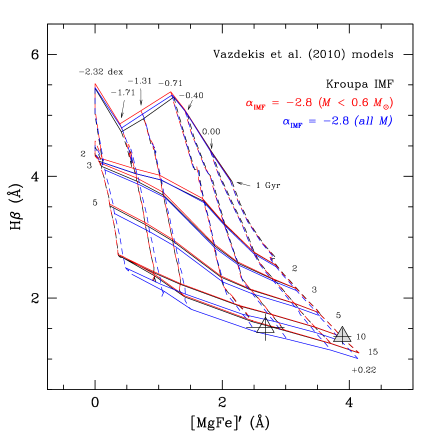
Figure 6.— H$\beta$ versus [MgFe]^′ for SSP model predictions of Vazdekis et al. (2010) using different IMFs (see legend on the right). Black lines: Kroupa (2001) IMF. Red lines: $\alpha=-2.8$ for ${\cal{M}}\leq 0.6\;M_{\odot}$ and Salpeter IMF for ${\cal{M}}>0.6\;M_{\odot}$. Blue lines: $\alpha=-2.8$ for all stellar masses. Dashed lines indicate [$Z$/H] values of $-$2.32, $-$1.71, $-$1.31, $-$0.71, $-$0.40, 0.00, and 0.22 dex. Solid lines indicate ages of 1, 2, 3, 5, 10, and 15 Gyr. For comparison, the grey and open triangles represent H$\beta$ and [MgFe]^′ at $R_{\rm gal}=50^{\prime\prime}$ for the diffuse light of NGC 4472 and NGC 1407, respectively. See the discussion in Sect. 4.3.

Similar conclusions can be drawn when comparing panels (e) – (g) with panel (h) of Figure 1 and panel (a) with panel (b) of Figure 2, except that the average colors of the red GC systems of the less luminous galaxies depicted there (see Table 1) are better matched by a slightly lower metallicity ($[Z/H]\simeq-0.2$). This is consistent with the color-magnitude relation among elliptical galaxies when interpreting color changes in terms of metallicity changes: the slope in the $V\!-\!K$ vs. $V$ relation among E galaxies in the Virgo galaxy cluster is $-0.079\pm 0.007$ (Bower et al., 1992), which translates to a [$Z$/H] vs. galaxy magnitude relation of $-$0.093 $\pm$ 0.008 dex/mag according to the Marigo et al. (2008) SSP models at an age of 12 Gyr.

A possible mechanism for producing the steep MFs in giant elliptical galaxies (relative to those of their massive red GCs) indicated by our results is discussed in the next Section.

5. Dynamical Evolution Effects on Stellar Mass Functions of Globular Clusters

The gradual disruption of star clusters over time affects the shape of their stellar MF, because the escape probability of stars from their parent cluster increases with decreasing stellar mass (e.g., Baumgardt & Makino, 2003). This effect has been used to explain the observed stellar MFs in ancient Galactic GCs, some of which are flatter than canonical IMFs (e.g., de Marchi et al., 2007; Paust et al., 2010). Such flat MFs in GCs can explain their low observed mass-to-light ratios when compared with predictions of SSP models that use canonical IMFs (e.g., Kruijssen & Mieske, 2009). The flattening of the MFs in Galactic GCs is greatest for GCs that are closest to dissolution (Baumgardt et al., 2008; Kruijssen, 2009).

Here, we explore the hypothesis that the IMF in the (high-metallicity, and likely high-density) environments that prevailed during the main star formation events that formed the stars in the bulge and the red GCs of giant elliptical galaxies was relatively steep ($-3.0\lesssim\alpha\lesssim-2.4$, as indicated by the analysis in the previous Section), i.e., steeper than the canonical IMF seen in the solar neighborhood, and that dynamical evolution of the star clusters formed during those events caused the stellar MF of the “average” surviving massive star cluster to be similar to a canonical IMF. To this end, we use the GC evolution model of Kruijssen (2009, hereafter K09) which incorporates the effects of stellar evolution, stellar remnant retention, dynamical evolution in a tidal field, and mass segregation. For the purposes of the current study, we select K09 models that (i) feature solar metallicity and “default” kick velocities of stellar remnants (white dwarfs, neutron stars, and black holes), and (ii) produce GCs with masses ${\cal{M}}_{\rm cl}\geq 2.5\times 10^{5}\>M_{\odot}$ at an age of 12 Gyr, i.e., the GCs shown in Figures 1 and 2 (cf. Section 2). We further consider King (1966) profiles with $W_{0}$ values of 5 and 7 and environmentally dependent cluster dissolution time scales $t_{0}$ of 0.3, 0.6, 1.0, and 3.0 Myr. For reference, $t_{0}=1.3$ Myr yields a reasonable fit to the globular cluster mass function of all (surviving) Galactic GCs (Kruijssen & Portegies Zwart, 2009).

Note however that GC systems in any given galaxy are expected to exhibit a range of $t_{0}$ values. For example, disruption rates of GCs in dense high-redshift environments were likely higher than in current quiescent galaxies (Kruijssen et al., 2012) due to the enhanced strength and rate of tidal perturbations. Likewise, GCs on eccentric orbits with smaller perigalactic distances $R_{\rm peri}$ should have smaller $t_{0}$ values than otherwise (initially) similar GCs with larger values of $R_{\rm peri}$. Finally, the rate of mass loss from GCs by evaporation, $\mu_{\rm ev}$, effectively scales with the mean GC half-mass density $\rho_{\rm h}$ as $\mu_{\rm ev}\propto\rho_{\rm h}^{0.5}$ for tidally limited GCs (e.g., McLaughlin & Fall 2008; Gieles et al. 2011; Goudfrooij 2012). Among GCs for which two-body relaxation has been the dominant mass loss mechanism, high-$\rho_{\rm h}$ GCs thus feature smaller $t_{0}$ values than low-$\rho_{\rm h}$ GCs at a given ${\cal{M}}_{\rm cl}$.

Figure 7 shows the present-day MF slopes $\alpha_{\it MF}$ in the stellar mass range 0.3 – 0.8 $M_{\odot}$ according to the K09 models for surviving GCs as a function of ${\cal{M}}_{\rm cl}$. The two panels (a) and (b) show the results for two different slopes of the stellar IMF: $\alpha_{\it IMF}=-3.00$ and $-2.35$, respectively. We also indicate “weighted mean” values of $\alpha_{\it MF}$ for a GC population with ${\cal{M}}_{\rm cl}\geq 2.5\times 10^{5}\;M_{\odot}$ at an age of 12 Gyr that was formed with a Schechter (1976) initial cluster mass function and a maximum initial mass of $10^{7}\>M_{\odot}$. For reference, a power-law fit to the Kroupa IMF in the mass range 0.3 – 0.8 $M_{\odot}$ yields $\alpha_{\it MF}=-1.7$ (cf. panels (d) and (h) of Fig. 1).

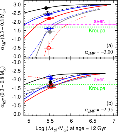
Figure 7.— Panel (a): MF slope $\alpha_{\it MF}$ in the range $0.3<{\cal{M}}_{\star}/M_{\odot}<0.8$ versus GC mass at an age of 12 Gyr for $\alpha_{\it IMF}=-3.00$ according to solar metallicity models of K09 that produce surviving GCs with ${\cal{M}}_{\rm cl}\geq 2.5\times 10^{5}\>M_{\odot}$ at an age of 12 Gyr. Solid lines represent models with King (1966) parameter $W_{0}=7$, while dashed lines do so for $W_{0}=5$. From top to bottom, the lines represent models with $t_{0}$ = 3.0, 1.0, 0.6, and 0.3 Myr (the latter only for $W_{0}=7$). Circles indicate weighted mean values for the abscissa and ordinate for each model, assuming a Schechter (1976) initial cluster mass function to assign weights and cluster masses $2.5\times 10^{5}\leq{\cal{M}}_{\rm cl}/M_{\odot}\leq 10^{7}$ at an age of 12 Gyr. The magenta dash-dotted line (along with an error bar) indicates the weighted average $\alpha_{\it MF}$ of all circles (using inverse variances as weights), while the green dotted line indicates the Kroupa IMF. Panel (b): Similar to panel (a), but now for a Salpeter (1955) IMF ($\alpha_{\it IMF}=-2.35$).

Focusing on the “weighted mean” values of $\alpha_{\it MF}$ for the K09 models shown in Figure 7, we find overall mean values $\overline{\alpha_{\it MF}}=-1.84\pm 0.26$ for $\alpha_{\it IMF}=-3.00$ and $\overline{\alpha_{\it MF}}=-1.80\pm 0.11$ for $\alpha_{\it IMF}=-2.35$, indicating that GCs with a steeper IMF experience a stronger evolution of the stellar MF. Note that both of these values are consistent with a Kroupa MF and hence consistent with the observed mean colors of red GCs shown in Figure 1. It is important to realize that the stronger flattening of $\alpha_{\it MF}$ over time in massive GCs with steeper IMFs is mainly caused by the weaker effect of retained massive stellar remnants on the escape rate of massive stars in GCs with steeper IMFs relative to that in GCs with flatter IMFs. As described in detail in K09, retained massive stellar remnants boost the escape rate of massive stars relative to that of low-mass stars. For a Kroupa IMF, this effect limits the flattening rate of $\alpha_{\it MF}$ over time relative to GCs with a lower fraction of massive stellar remnants (see K09). However, GCs with steeper IMFs feature a smaller mass fraction taken up by massive remnants. This notably reduces the ‘dampening effect’ of retained massive remnants on the evolution of $\alpha_{\it MF}$. As a result, the present-day stellar MFs in GCs are consistent with any IMF slope $\alpha\lesssim-1.7$. This degeneracy implies that the IMF cannot be uniquely constrained in this range for individual GCs. However, the large spread of observed MF slopes among Galactic GCs (de Marchi et al., 2007; Paust et al., 2010) seems to be more consistent with a bottom-heavy IMF (compare both panels in Figure 7).

We conclude that the difference in $g\!-\!z$ or $B\!-\!I$ color between giant elliptical galaxies and their “average” massive red GCs shown in Figures 1 and 2 is consistent with long-term dynamical evolution of star clusters that were formed with a steeper IMF than those derived from star counts in the solar neighborhood. Among the three mechanisms we think could conceivably cause this color difference, this is the only one that seems consistent with the data. Hence we suggest that this color difference constitutes evidence for a “bottom-heavy” IMF in luminous elliptical galaxies.

6. Discussion

Our results add to a developing consensus that luminous elliptical galaxies have “heavy” IMFs, with a greater contribution from low-mass dwarf stars than IMFs determined from star count studies in the Milky Way. Cenarro et al. (2003) studied the Ca ii triplet near 8600 Å, which is stronger in RGB stars than in MS stars, in a sample of elliptical galaxies. They found that the strength of the Ca ii triplet decreases with increasing velocity dispersion among elliptical galaxies. This is hard to explain in terms of an Ca abundance trend since Ca is an $\alpha$ element, and [$\alpha$/Fe] as derived from Mg and Fe features near 5200 Å does not show this trend. Hence, they suggested that this trend might reflect an increasing IMF slope with increasing galaxy mass, as indicated by SSP models of Vazdekis et al. (2003). Similarly, van Dokkum & Conroy (2010, 2011) found strong equivalent widths of the Na i $\lambda\lambda 8183,8195$ doublet and the molecular FeH band at 9916 Å in near-IR spectra of giant elliptical galaxies. As both of those indices are stronger in red dwarf stars than in red giants, their strongly favored explanation is the presence of a significantly larger number of late M dwarf stars than that implied by a Kroupa IMF, even though there is a slight degeneracy with [Na/Fe] ratio (see also Conroy & van Dokkum, 2012; Smith et al., 2012). Finally, Cappellari et al. (2012) studied stellar ${\cal{M}}/L$ ratios [$({\cal{M}}/L)_{\rm stars}$] derived from integral-field spectroscopy of 260 early-type galaxies. They found that the ratio of $({\cal{M}}/L)_{\rm stars}$ by the ${\cal{M}}/L$ predicted by SSP models that use a Salpeter IMF $[({\cal{M}}/L)_{\rm Salp}]$ varies systematically with galaxy velocity dispersion: galaxies with the largest values of $({\cal{M}}/L)_{\rm stars}/({\cal{M}}/L)_{\rm Salp}$ have the highest velocity dispersions (see also Tortora et al., 2012). However, dynamical modeling such as that done by Cappellari et al. (2012) cannot unambiguously constrain whether the highest values of $({\cal{M}}/L)_{\rm stars}/({\cal{M}}/L)_{\rm Salp}$ are due to a large population of low-mass stars (i.e., a bottom-heavy IMF) or large number of massive stellar remnants (i.e., a top-heavy IMF). The same degeneracy is present for mass estimates from gravitational lensing (e.g., Treu et al., 2010). In contrast, our results indicate that the bottom-heavy IMF is the more likely solution.

Finally, we review the dependence of our results on SSP model ingredients. At old ages ($\gtrsim 10$ Gyr) and high metallicities ([$Z$/H] $\gtrsim-0.5$), SSP models still suffer from several limitations. The likely most significant internal uncertainty is related to lifetimes of AGB stars (see, e.g., Melbourne et al., 2012). In terms of external uncertainties, we note that integrated colors and spectral indices of several SSP models are calibrated to observations of the two Galactic bulge GCs NGC 6528 and NGC 6553 that have $Z\simeq Z_{\odot}$ (e.g., Thomas et al., 2003; Maraston, 2005). However, there are no published MFs for those two GCs available to our knowledge, yielding an uncertainty in the absolute calibration. Notwithstanding such limitations, our main result is based on $g\!-\!z$ or $B\!-\!I$ color differences between the average red massive GC and their parent galaxies and the absence of such differences in H$\beta$ and [MgFe]^′ indices. As the interpretation of relative colors or line strengths should be largely model-independent, our result strongly suggests a bottom-heavy IMF in massive elliptical galaxies.

Appendix A Building synthetic integrated colors of metal-rich globular clusters containing two stellar generations

In this appendix, we determine colors of various stellar types from synthetic spectra with chemical compositions typical of first– and second-generation stars found in massive metal-rich GCs. We assume [Z/H] = 0.0 and explore two choices for the abundances of He, C, N, O, and Na. To simulate first-generation (FG) stars, we choose the primordial He abundance ($Y$ = 0.235 + 1.5 $Z$), we follow Cannon et al. (1998) by choosing [C/Fe] = 0.06 and [N/Fe] = 0.20, and we adopt [O/Fe] = 0.40 and [Na/Fe] = 0.00 from Carretta et al. (2009). To simulate second-generation (SG) stars, we choose [C/Fe] = $-$0.15, [N/Fe] = 1.05, [O/Fe] = $-$0.10, and [Na/Fe] = 0.60 (see Carretta et al., 2009). For the He abundance of SG stars, we consider the case of NGC 6441, a metal-rich GC in the bulge of our Galaxy ([Fe/H] = $-$0.59, Zinn & West, 1984). NGC 6441 (as well as the similar cluster NGC 6388) is unusual among metal-rich GCs in our Galaxy in that it shows a horizontal branch (HB) that extends blueward of the RR Lyrae instability strip in the CMD whereas all other metal-rich GCs have purely red HBs (e.g., Rich et al., 1997). The blueward extension of the HB of NGC 6441 is widely thought to be due to enhanced He in a fraction of its constituent stars, and we adopt the value $Y=0.33$ from Caloi & D’Antona (2007). As blue HBs are very unusual among massive metal-rich GCs in our Galaxy, this value of $Y$ should probably be considered an upper limit for SG stars in the context of the current paper.

To produce synthetic integrated colors of stellar populations, we first build two sets of synthetic spectra for six stellar types that span almost the full range of luminosities $L$ and temperatures $T_{\rm eff}$ encompassed by the isochrones (see Figure 8). For this purpose we select Dartmouth isochrones (Dotter et al., 2007) with [Z/H] = 0.0, [$\alpha$/Fe] = +0.4, and the two values of $Y$ mentioned in the previous paragraph. [Z/H] values for alpha-enhanced populations are evaluated using [Z/H] = [Fe/H] + 0.929 [$\alpha$/Fe] (Trager et al., 2000). The parameters of the model atmospheres are listed in Table 2. These temperatures, gravities, and chemical abundances are then used to calculate model atmospheres and synthetic spectra using the codes ATLAS12 and SYNTHE (Kurucz, 2005; Castelli, 2005; Sbordone et al., 2007), respectively. ATLAS12 allows one to use arbitrary chemical compositions. In doing so, we use model atmospheres from the [Fe/H] = 0.0, [$\alpha$/Fe] = +0.4 model grid of Castelli & Kurucz (2004) as reference and adjust $T_{\rm eff}$, $g$, [Fe/H], and the individual element abundances in the ATLAS12 runs. The resulting synthetic spectra are then redshifted according to the heliocentric radial velocity of the Virgo galaxy cluster (1035 km s^-1, Mould et al., 2000) and integrated over passbands of Johnson/Cousins ($U_{J}$, $B_{J}$, $V_{J}$, $R_{C}$, $I_{C}$; Bessell, 1990) and Sloan ugriz to produce synthetic magnitudes and colors.

Figure 8.— Theoretical isochrones from the lower MS to the upper RGB for the two different chemical compositions associated with two stellar generations within massive GCs. The solid line corresponds to the first-generation population (with primordial He abundance), whereas the dashed line corresponds to the second-generation population (with enhanced He abundance $Y$ = 0.33). The filled and open squares indicate the stellar types for which we calculated model atmospheres and synthetic spectra (cf. Table 2). See text for more details.

Table 2Stellar parameters of the model atmospheres.

$T_{\rm eff}$ (FG)	$T_{\rm eff}$ (SG)	log $g$	$V_{\rm turb}$
(1)	(2)	(3)	(4)
3602	3665	4.79	2.0
4526	4795	4.59	2.0
5630	5700	4.20	2.0
4835	4941	3.48	2.0
4237	4311	1.96	2.0
3537	3608	0.70	2.0

Three examples of the synthetic spectra for FG and SG stars are shown in Figs. 9 – 11. Labels in each plot indicate prominent absorption features that change significantly in strength between the two chemical compositions. These spectra are described briefly below.

Figure 9 compares RGB spectra of the FG and SG mixtures. The higher [N/Fe] of the SG mixture causes stronger molecular bands of CN. This is especially clear at $\lambda\gtrsim 7000$ Å. The main reason why this is not as obvious for the CN bands near 3590, 3883, and 4150 Å and the NH band near 3360 Å is that the enhanced absorption in the blue region for the SG mixture is partially compensated by its enhanced He abundance which elevates the stellar continuum in the blue. The increased opacity at $\lambda\lesssim 4500$ Å for the SG mixture also causes a somewhat elevated stellar continuum at longer wavelengths, which likely causes the slightly higher flux of the SG mixture in the 4500 – 6200 Å region. Finally, the lower O abundance of the SG mixture causes a weaker OH absorption band between 3050 and 3200 Å which just falls within the $U_{J}$ and $u$ bands for the radial velocities of the galaxies in our sample.

In the spectra of TO stars (Figure 10), the higher temperature causes generally weaker molecular bands, rendering generally small differences between the FG and SG spectra. Only the NH and CN bands remain slightly stronger in the SG mixture.

The differences between the FG and SG spectra of cool MS stars (Figure 11) are generally similar to those seen for the RGB spectra, except that the MS stars show weaker red CN bands and a slightly stronger OH band in the 3000 – 3200 Å region.

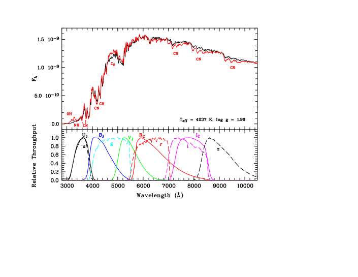
Figure 9.— Top panel: Synthetic spectra for RGB models with log $g$ = 1.96 for the FG (black) and SG (red) mixtures. The spectra were convolved with a Gaussian with $\sigma$ = 12 Å to improve readability. Relevant molecular bands are labelled. Bottom panel: Transmission curves for Johnson/Cousins $U_{J}$, $B_{J}$, $V_{J}$, $R_{C}$, and $I_{C}$ filters (solid curves, left to right) and SDSS ugriz filters (dashed curves). See text for details.

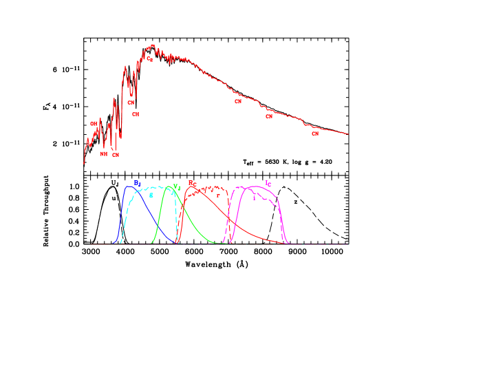
Figure 10.— Like Figure 9, but now for TO models with log $g$ = 4.20.

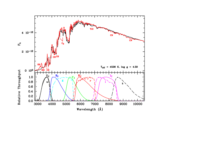
Figure 11.— Like Figure 9, but now for MS models with log $g$ = 4.59.

Differences in stellar absolute magnitude $\Delta M\equiv M_{\rm SG}-M_{\rm FG}$ are then evaluated as a function of log $g$ for all filter passbands considered here. The results are illustrated in Figure 12 which shows $\Delta M$ as a function of log $g$. The largest differences show up in the $U_{J}$ and $u$ passbands, due to their sensitivity to relevant parameters: (i) $T_{\rm eff}$ and hence $Y$; (ii) N abundance through the NH band near 3360 Å as well as the CN bands near 3590 and 3883 Å; and (iii) O abundance through the OH band at the short-wavelength edge of the $U_{J}$ and $u$ filters. The weaker OH absorption for the SG population is the main reason why $\Delta M$ for the $U_{J}$ and $u$ passbands is negative at the top of the RGB (i.e., lowest log $g$). $\Delta M$ then increases significantly with increasing log $g$ to become positive at the TO (due mainly to stronger NH and CN absorption in the SG population), and then decreases again to the bottom of the MS (i.e., highest log $g$). The other passbands (longward of $\sim 4000$ Å) show a similar dependence of $\Delta M$ on log $g$, although the absolute $\Delta M$ values at $\lambda\gtrsim 4000$ Å are much smaller than for $U_{J}$ and $u$ at a given log $g$.

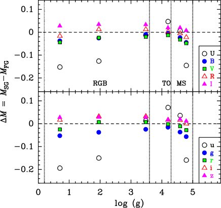
Figure 12.— Differences between stellar absolute magnitudes of the FG and SG stars considered in this paper as a function of log $g$. Upper panel: Johnson/Cousins UBVRI filters (see legend for symbols). Lower panel: Sloan ugriz filters. Dashed vertical lines delineate the RGB, TO, and MS regions on the CMD (see labels near the bottom of the upper panel). See Appendix A for more details.

The dependence of $\Delta M$ between FG and SG populations as a function of wavelength found here are qualitatively similar to those of Sbordone et al. (2011) who did a similar study at low metallicity ([Fe/H] = $-$1.62). However, we find that $\Delta M$ values are different for metal-rich populations in a quantitative sense, sometimes by a significant amount.

Isochrone tables for the SG population are then calculated by adding $\Delta M$ to the absolute magnitudes for each filter passband in the (FG) isochrone tables (i.e., $M_{\rm SG}=M_{\rm FG}+\Delta M$), using linear interpolation in log $g$. After rebinning the resulting isochrone tables to a uniform bin size in stellar mass using linear interpolation, weighted integrated luminosities of the population were derived for the relevant passbands by weighting individual stellar luminosities in the isochrones using a “standard” Kroupa (2001) IMF. Resulting integrated-light magnitude offsets (in the sense SG $-$ FG) are listed for each filter passband in Table 3. Interestingly, the large differences found in the $U_{J}$ and $u$ passbands between FG and SG populations at a given stellar type largely cancel out in integrated light (i.e., when integrated over the stellar mass function). Integrated-light magnitude offsets are found to stay within 0.03 mag in an absolute sense for any of the filter passbands considered here. Finally, and in the context of the subject of this paper, we note that the resulting offsets between SG and FG populations in the $B\!-\!I$ and $g\!-\!z$ colors are $-$0.041 and $-$0.054 mag (in the sense SG $-$ FG), respectively. Since recent multi-object spectroscopy studies of massive Galactic GCs typically show an approximate 50 – 50% split between FG and SG stars (e.g., Gratton et al., 2012), we conclude that the predicted overall effect of the presence of multiple stellar generations on the integrated $B\!-\!I$ and $g\!-\!z$ colors of massive metal-rich GCs is offsets of $-$0.021 and $-$0.027 mag, respectively.

Table 3Integrated-light magnitude offsets between the SG and FG populations.

$\Delta U_{J}$	$\Delta B_{J}$	$\Delta V_{J}$	$\Delta R_{C}$	$\Delta I_{C}$
$+$0.002	$-$0.018	$-$0.027	$-$0.002	$+$0.023
$\Delta u$	$\Delta g$	$\Delta r$	$\Delta i$	$\Delta z$
$+$0.022	$-$0.031	$-$0.007	$+$0.018	$+$0.023

References

- Ashman et al. (1994) Ashman, K. M., Bird, C. M., & Zepf, S. E. 1994, AJ, 108, 2348
- Bassino et al. (2006) Bassino, L. P., Faifer, F. R., Forte, J. C., et al. 2006, A&A, 451, 789
- Bastian et al. (2010) Bastian, N., Covey, K. R., & Meyer, M. R. 2010, ARA&A, 48. 339
- Baumgardt & Makino (2003) Baumgardt, H., & Makino, J. 2003, MNRAS, 340, 227
- Baumgardt et al. (2008) Baumgardt, H., de Marchi, G., & Kroupa, P. 2008, ApJ, 685, 247
- Bessell (1990) Bessell, M. S. 1990, PASP, 102, 1181
- Bower et al. (1992) Bower, R. G., Lucey, J. R., & Ellis, R. S. 1992, MNRAS, 254, 601
- Brodie & Strader (2006) Brodie, J. P., & Strader, J. 2006, ARA&A, 44, 193
- Brodie et al. (2005) Brodie, J. P., Strader, J., Denicoló, G., et al. 2005, AJ, 129, 2643
- Brodie et al. (2012) Brodie, J. P., Usher, C., Conroy, C., et al. 2012, ApJ, in press (arXiv:1209.5390)
- Caloi & D’Antona (2007) Caloi, V., & D’Antona, F. 2007, A&A, 463, 949
- Cannon et al. (1998) Cannon, R. D., Croke, B. F. W., Bell, R. A., Hesser, J. E., & Stathakis, R. A., 1998, MNRAS, 298, 601
- Cappellari et al. (2012) Cappellari, M., McDermid, R. M., Alatalo, K., et al. 2012, Nature, 484, 485
- Carretta et al. (2009) Carretta, E., Bragaglia, A., Gratton, R. G., et al. 2009, A&A, 505, 117
- Carretta et al. (2010) Carretta, E., Bragaglia, A., Gratton, R. G., et al. 2010, A&A, 516, A55
- Castelli (2005) Castelli, F. 2005, Mem. Soc. Astron. Ital. Supp., 8, 25
- Castelli & Kurucz (2004) Castelli, F., & Kurucz, R. L. 2004, [arXiv:astro-ph/0405087]
- Chabrier (2003) Chabrier, G. 2003, PASP, 115, 763
- Chies-Santos et al. (2011) Chies-Santos, A. L., Larsen, S. S., Kuntschner, H., et al. 2011, A&A, 525, A20
- Cenarro et al. (2003) Cenarro, A. J., Gorgas, J., Vazdekis, A., Cardiel, N., & Peletier, R. F., 2003, MNRAS, 339, L12
- Cenarro et al. (2007) Cenarro, A. J., Beasley, M. A., Strader, J., Brodie, J. P., & Forbes, D. A. 2007, AJ, 134, 391
- Cerviño & Luridiana (2004) Cerviño, M., & Luridiana, V. 2004, A&A, 413, 145
- Cohen et al. (2003) Cohen, J. G., Blakeslee, J. P., & Côté, P. 2003, ApJ, 592, 866
- Conroy & van Dokkum (2012) Conroy, C., & van Dokkum, P. G. 2012, submitted to ApJ (arXiv:1205.6473)
- Côté et al. (2004) Côté, P., Blakeslee, J. P., Ferrarese, L., et al. 2004, ApJS, 153, 223
- Davies et al. (1993) Davies, R. L., Sadler, E. M., & Peletier, R. F. 1993, MNRAS, 262, 650
- de Marchi et al. (2007) de Marchi, G., Paresce, F., & Pulone, L. 2007, ApJ, 656, L65
- Dotter et al. (2007) Dotter, A., Chaboyer, B., Jevremović, D., et al. 2007, AJ, 134, 476
- Dotter et al. (2010) Dotter, A., Sarajedini, A., & Anderson, J., et al. 2010, ApJ, 708, 698
- Elmegreen & Efremov (1997) Elmegreen, B. G., & Efremov, Yu. N. 1997, ApJ, 480, 235
- Ferrarese et al. (2006) Ferrarese, L., et al. 2006, ApJS, 164, 334
- Fisher et al. (1995) Fisher, D., Franx, M., & Illingworth, G. 1995, ApJ, 448, 119
- Forbes et al. (2006) Forbes, D. A., Sánchez-Blázquez, P., Phan, A. T. T., et al. 2006, MNRAS, 366, 1230
- Geisler et al. (1996) Geisler, D., Lee, M. G., & Kim, E. 1996, AJ, 111, 1529
- Georgiev et al. (2009) Georgiev, I. Y., Hilker, M., Puzia, T. H., Goudfrooij, P., & Baumgardt, H. 2009, MNRAS, 396, 1075
- Gieles et al. (2011) Gieles, M., Heggie, D. C., & Zhao, H. 2011, MNRAS, 413, 2509
- Goudfrooij (2012) Goudfrooij, P. 2012, ApJ, 750, 140
- Goudfrooij et al. (2007) Goudfrooij, P., Schweizer, F., Gilmore, D., & Whitmore, B. C. 2007, AJ, 133, 2737
- Gratton et al. (2012) Gratton, R. G., Carretta, E., & Bragaglia, A. 2012, A&A Rev., 20, 50
- Johnson & Pilachowski (2010) Johnson, C. I., & Pilachowski, C. A. 2010, ApJ, 722, 1373
- Jordán et al. (2007) Jordán, A., McLaughlin, D. E., Côté, P., et al. 2007, ApJS, 171, 101
- Jordán et al. (2009) Jordán, A., Peng, E. W., Blakeslee, J. P., et al. 2009, ApJS, 180, 54
- King (1966) King, I. R. 1966, AJ, 71, 64
- Kravtsov et al. (2011) Kravtsov, V., Alcaíno, G., Marconi, G., & Alvarado, F. 2011, A&A, 527, L9
- Kroupa (2001) Kroupa, P. 2001, MNRAS, 322, 231
- Kruijssen (2009) Kruijssen, J. M. D. 2009, A&A, 507, 1409
- Kruijssen & Mieske (2009) Kruijssen, J. M. D., & Mieske, S. 2009, A&A, 500, 785
- Kruijssen & Portegies Zwart (2009) Kruijssen, J. M. D., & Portegies Zwart, S. F. 2009, ApJ, 698, L158
- Kruijssen et al. (2012) Kruijssen, J. M. D., Pelupessy, F. I., Lamers, H. J. G. L. M., et al. 2012, MNRAS, 421, 1927
- Kruijssen (2012) Kruijssen, J. M. D. 2012, MNRAS, 426, 3008
- Kundu & Whitmore (2001) Kundu, A., & Whitmore, B. C. 2001, AJ, 121, 1888
- Kundu et al. (2005) Kundu, A., et al. 2005, ApJ, 634, L41
- Kurucz (2005) Kurucz, R. L. 2005, Mem. Soc. Astron. Ital. Supp., 8, 14
- Lada & Lada (2003) Lada, C. J., & Lada, E. A. 2003, ARA&A, 41, 57
- Larsen et al. (2003) Larsen, S. S., et al. 2003, ApJ, 585, 767
- Lee et al. (2007) Lee, Y.-W., Gim, H. B., & Casetti-Dinescu, D. I. 2007, ApJ, 661, L49
- Lee et al. (2005) Lee, Y., Joo, S., Han, S., et al. 2005, ApJ, 621, L57
- Liu et al. (2011) Liu, C., et al. 2011, ApJ, 728, 116
- Maraston (2005) Maraston, C. 2005, MNRAS, 362, 799
- Marino et al. (2008) Marino, A. F., Villanova, S., Piotto, G., et al. 2008, A&A, 490, 625
- Marino et al. (2009) Marino, A. F., Sneden, C., Kraft, R. P., et al. 2011, A&A, 532, A8
- Marigo et al. (2008) Marigo, P., Girardi, L., Bressan, A., et al. 2008, A&A, 482, 883
- McLachlan & Basford (1988) McLachlan, G. J., & Basford, K. E. 1988, Mixture Models: Inference and Application to Clustering (New York: M. Dekker)
- McLaughlin & Fall (2008) McLaughlin, D. E., & Fall S. M. 2008, ApJ, 679, 1272
- Melbourne et al. (2012) Melbourne, J., Williams, B. F., Dalcanton, J. J., et al. 2012, ApJ, 748, 47
- Milone et al. (2012) Milone, A. P., Piotto, G., Bedin, L. R., et al. 2012, ApJ, 744, 58
- Mould et al. (2000) Mould, J. R., Huchra, J. P., Freedman, W. L., et al. 2000, ApJ, 529, 786
- Paust et al. (2010) Paust, N. E. Q., et al. 2010, AJ, 139, 476
- Peng et al. (2006) Peng, E. W., et al. 2006, ApJ, 639, 95
- Portegies Zwart et al. (2010) Portegies Zwart, S. F., McMillan, S. L. W., & Gieles, M. 2010, ARA&A, 48, 431
- Puzia et al. (2002) Puzia, T. H., Zepf, S. E., Kissler-Patig, M., Hilker, M., Minniti, D., & Goudfrooij, P. 2002, A&A, 391, 453
- Puzia et al. (2005) Puzia, T. H., Kissler-Patig, M., Thomas, D., et al. 2005, A&A, 439, 997
- Puzia et al. (2006) Puzia, T. H., Kissler-Patig, M., & Goudfrooij, P. 2006, ApJ, 648, 383
- Renzini (2008) Renzini, A. 2008, MNRAS, 391, 354
- Rhode & Zepf (2001) Rhode, K. L., & Zepf, S. E. 2001, AJ, 121, 210
- Rich et al. (1997) Rich, R. M., Sosin, C., Djorgovski, S. G., et al. 1997, ApJ, 484, L25
- Salpeter (1955) Salpeter, E. E. 1955, ApJ, 121, 161
- Sbordone et al. (2007) Sbordone, L., Bonifacio, P., & Castelli, F. 2007, Proc. IAU Symp. 239, Convection in Astrophysics, ed. F. Kupka, I. W. Roxburgh, & K. L. Chan (Cambridge: Cambridge Univ. Press), 71
- Sbordone et al. (2011) Sbordone, L., Salaris, M., Weiss, A., & Cassisi, S. 2011, A&A, 435, A9
- Schechter (1976) Schechter, P. 1976, ApJ 203, 297
- Smith et al. (2012) Smith, R. J., Lucey, J. R., & Carter, D. 2012, MNRAS, in press (arXiv:1206.4311)
- Spolaor et al. (2008a) Spolaor, M., Forbes, D. A., Hau, G. K. T., Proctor, R. N., & Brough, S. 2008a, MNRAS, 385, 667
- Spolaor et al. (2008b) Spolaor, M., Forbes, D. A., Proctor, R. N., Hau, G. K. T., & Brough, S. 2008b, MNRAS, 385, 675
- Tortora et al. (2012) Tortora, C., Romanowsky, A. J., & Napolitano, N. R. 2012, ApJ, in press (arXiv:1207.4475)
- Trager et al. (2000) Trager, S. C., Faber, S. M., Worthey, G., & González, J. J. 2000, AJ, 120, 165
- Treu et al. (2010) Treu, T., Auger, M. W., Koopmans, L. V. E., et al. 2010, ApJ, 709, 1195
- Thomas et al. (2003) Thomas, D., Maraston, C., & Bender, R. 2003, MNRAS, 339, 897
- van Dokkum & Conroy (2010) van Dokkum, P. G., & Conroy, C. 2010, Nature, 468, 940
- van Dokkum & Conroy (2011) van Dokkum, P. G., & Conroy, C. 2011, ApJ, 735, L13
- Vazdekis et al. (2003) Vazdekis, A., Cenarro, A. J., Gorgas, J., Cardiel, N., & Peletier, R. F., 2003, MNRAS, 340, 1317
- Vazdekis et al. (2010) Vazdekis, A., Sánchez-Blázquez, P., Falcón-Barroso, J., et al. 2010, MNRAS, 404, 1639
- Worthey (1994) Worthey, G. 1994, ApJS, 95, 107
- Zinn & West (1984) Zinn, R. J., & West, M. J. 1984, ApJS, 55, 45